Analytical study of atmospheric internal waves model with fractional approach

Trushit Patel; Hardik Patel; Ramakanta Meher

doi:10.1016/j.joes.2022.02.004

Journal of Ocean Engineering and Science >

2024 , Vol. 9 >Issue 4: 326 - 335

DOI: https://doi.org/10.1016/j.joes.2022.02.004

Original article

Analytical study of atmospheric internal waves model with fractional approach

Trushit Patel ^,^a ,
Hardik Patel ^,^b ,
Ramakanta Meher ^,^c

Expand

^a Computer Science, University of the People, Pasadena, CA 91101, United States
^b Department of Mathematics, Uka Tarsadia University, Bardoli, Gujarat, India
^c Mathematics and Humanities Department, Sardar Vallabhbhai National Institute of Technology, Surat, Gujarat, India

Received 9 December 2021, Revised 23 January 2022, Accepted 10 February 2022, Available online 17 February 2022, Version of Record 22 July 2024. E-mail:trushitkumar.patel@uopeople.edu;hardik.spatel@utu.ac.in;meher_ramakanta@yahoo.com

Received date: 2021-12-09

Revised date: 2022-01-23

Accepted date: 2022-02-10

Online published: 2024-08-13

Fold

Abstract

This study looks at the mathematical model of internal atmospheric waves, often known as gravity waves, occurring inside a fluid rather than on the surface. Under the shallow-fluid assumption, internal atmospheric waves may be described by a nonlinear partial differential equation system. The shallow flow model's primary concept is that the waves are spread out across a large horizontal area before rising vertically. The Fractional Reduced Differential Transform Method(FRDTM) is applied to provide approximate solutions for any given model. This aids in the modelling of the global atmosphere, which has applications in weather and climate forecasting. For the integer-order value (Î±=1), the FRDTM solution is compared to the precise solution, EADM, and HAM to assess the correctness and efficacy of the proposed technique.

Highlights

● Under the shallow fluid assumption, the mathematical model of internal atmospheric waves is considered.

● In this model, waves are spread out across a large horizontal area before rising vertically.

● The fractional reduced differential transform method (FRDTM) is applied to find the approximate solution of time-fractional non-linear system of PDEs.

● The fractional solution provides a pragmatic look into the physical behaviour of internal waves, which can be helpful to refine climate and weather models.

● The obtained results have been compared with the numerical solution, EADM, and HAM for integer order to check the correctness and efficacy of the proposed technique.

Key words： Shallow-fluid equations; Atmospheric internal waves; Time-fractional partial differential equations; Fractional reduced differential transform method (FRDTM); Climate prediction

Cite this article

Trushit Patel , Hardik Patel , Ramakanta Meher . Analytical study of atmospheric internal waves model with fractional approach[J]. Journal of Ocean Engineering and Science, 2024 , 9(4) : 326 -335 . DOI: 10.1016/j.joes.2022.02.004

1. Introduction

Internal waves are disturbances that flow through fluid interfaces and diseases that migrate along the pycnocline. Internal waves in the water cause a slight vertical movement of the free surface, making them invisible to floating structures. These waves are difficult to detect, although they have been observed, even in very rough waters. Pycnocline and thermocline are the two sudden changes in water density and temperature that occur around 50 m below the surface. A progressive contact between two fluids of various thicknesses is known as pycnocline. These waves might be rather large. Since internal waves are not immediately visible, they can only be identified by their surface signature and direct measurements of the pycnocline or thermocline. The waves can be determined by the increased roughness of the ocean surface when the density interface is shallow enough to allow the internal wave crests to contact the sea surface. Internal waves are vital in the mixing of various levels of water in the seas, which impacts climate. One of the most significant areas of uncertainty in current climate models, is the pace of such mixing [1].

Fig. 1 depicts the internal wave phenomenon in different locations of the world. Water propagates beneath the surface, so it can't be seen or measured directly, but it leaves a distinct trail on the surface that can be detected by satellites. Internal waves in the South China Sea were photographed by NASA's shuttle in June 1983, and on the coast of Peru in 1984. According to investigations conducted over the last decade, internal waves have a binding influence on chemistry, ambient temperature, and turbulence. Internal airwaves are often represented using shallow-fluid equations, also known as shallow water equations.

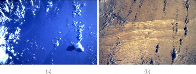
View original graphic|Download|PPT slide

Fig.1 Internal waves in (a) south china sea (STS-7, June 1983, picture-#7-05-0245) and (b) Eastern Pacific Sea (STS-41C, April 1984, picture-#13-31-980).

The internal waves phenomenon has been discussed by researchers from various viewpoints and many analytical and numerical methods have been used to get solutions to understand the behaviour of the model. Le Roux et al. [2] applied finite-element spatial discretization to solve shallow water equation, ocean models. Aguilar and Sutherland [3] examined internal wave generation from periodic topography having various degrees of roughness through laboratory experiments. Boyd and Zhou [4] studied the Kelvin waves which are the lowest eigenmode of Laplace's tidal equation in non-linear shallow water equations on the sphere. Imani et al. [5] used the reconstruction variational iteration (RVI) method for solving the coupled Whitham-Broer-Kaup shallow water wave equation. Chakraverty and Karunakar [6] applied the homotopy perturbation method (HPM) to obtain an analytical solution of linear as well as non-linear shallow water wave equations. Jaharuddin and Hermansyah [7] used the homotopy analysis method (HAM) to study the internal ocean waves caused by the tidal force. Busrah et al. [8] obtained the analytical solution of the internal atmospheric waves by using the HAM and variational iteration method (VIM). Varsoliwala and Singh [9] investigated tsunami wave propagation in the mid-ocean and addressed its run-up and amplification on land; they [10] used EADM to investigate internal atmospheric waves.

The shallow-fluid model's fundamental assumption is that the horizontal dimension is significantly more than the vertical. The schematic representation of internal waves is shown in Fig. 2. Nonlinear partial differential equations, called shallow water equations are used to explain fluid flows in seas, coastal regions, and the atmosphere. The next step is to apply the analytical and numerical methods developed in this study to make more specific predictions about ocean regions, which will then be tested in the field. The fading of internal waves is a fundamental subject that is largely unanswered till date.

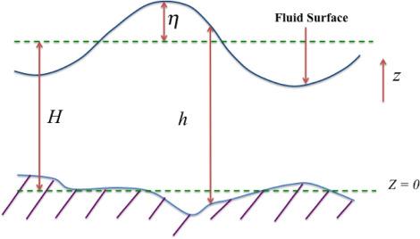
View original graphic|Download|PPT slide

Fig.2 Schematic representation of internal waves.

Any real-world situation that is studied yields an equation, and the number of parameters involved in such problems cause partial differential equations (PDEs). Furthermore, many real-world events are governed by integer-order PDEs that are difficult to explain. As a result, fractional-order nonlinear PDEs add to the importance of the study. Many analytical, numerical, and transform approaches are used to solve fractional order systems of linear and nonlinear PDEs. The ADSTM was utilized by Patel and Meher [11], [12] to investigate the fractional-order energy balance equation originating from heat transport through fins. Goswami et al. [13] used the analytical method HPSTM to investigate fractional partial differential equations that arise in plasma ion-acoustic waves. On the fractional Kakutani Matsu chi, water wave model, Moradi, and Sayevand [14] used an effective numerical methodology called the finite difference method. Using FRDTM, Tandel et al. [15] investigated the frictional behaviour of the tsunami wave propagation model. In applied sciences, Tamboli and Tandel [16] employed FRDTM to solve the time-fractional generalized Burger-Fisher equation, a governing equation in various applications such as gas dynamics simulation, fluid mechanics, financial mathematics, and ocean engineering. Using the solution approach, Dassios and Font [17] explored three definitions of fractional derivatives to get an analytical solution of the time-fractional hyperbolic heat equation.

The primary purpose of this paper is to analyze the behaviour of fractional-order shallow fluid equation using the latest analytical method FRDTM and show the applications to the time fractional-order atmospheric internal waves model that propagates within a medium of fluid which is the novelty of this work. Also, FRDTM provides highly accurate numerical results without spatial discretization, linearization, transformation, or perturbation for nonlinear time-fractional differential equations and this method can be applied to derive a variety of fractional-order non-linear problems with distinct physical structures arising in ocean engineering-related problems.

2. Mathematical model formulation

Internal waves in the atmosphere are modelled by a system of non-linear PDEs based on the shallow fluid assumption. By using mass and momentum conservation, the primary equations of the motion of fluid in differential form can be obtained. The term "shallow fluid" refers to a fluid layer with a shallow depth compared to its height. The atmosphere is supposed to be a homogeneous fluid whose density does not change with space, autobarotropic whose density is only determined by inviscid, hydrostatic, pressure, and incompressible fluid. The followings are the fundamental momentum equations [18].

(1)

\begin{matrix} M_{t} + M M_{x} + P M_{y} + Q M_{z} = F P - \frac{1}{ρ} {\tilde{P}}_{x}, \end{matrix}

(2)

\begin{matrix} P_{t} + M P_{x} + P P_{y} + Q P_{z} = - F M - \frac{1}{ρ} {\tilde{P}}_{y}, \end{matrix}

(3)

\begin{matrix} {\tilde{P}}_{z} = - ρ G, \end{matrix}

The equation for continuity is

(4)

\begin{matrix} ρ_{t} + ρ (M_{x} + P_{y} + Q_{z}) = 0, \end{matrix}

When fluid is incompressible and homogeneous then

(5)

\begin{matrix} ρ_{t} = 0, \end{matrix}

i.e.,

ρ = ρ_{0}

is a constant. Therefore, Eq. (4) can be written as

(6)

\begin{matrix} M_{x} + P_{y} + Q_{z} = 0, \end{matrix}

The equation of hydrostatic can be written as

(7)

\begin{matrix} {\tilde{P}}_{z} + ρ_{0} G = 0, \end{matrix}

we get

(8)

\begin{matrix} {({\tilde{P}}_{z})}_{x} = {({\tilde{P}}_{x})}_{z} = 0, \end{matrix}

As a result of barotropy, there is no horizontal variation of the vertical pressure gradient or vice versa. All types of forces are invariable with depth, such as the resulting Coriolis force and the wind created by the pressure-gradient force.

Integrating the Eq. (7) across the fluid's depth

(9)

\begin{matrix} \int_{z (V_{B})}^{z (V_{T})} ({\tilde{P}}_{z}) d z + ρ_{0} G \int_{z (V_{B})}^{z (V_{T})} d z = 0, \end{matrix}

where

V_{T}

and

V_{B}

are the pressures at the fluid's top and bottom edges, respectively.

(10)

\begin{matrix} V_{B} - V_{T} = ρ_{0} G Z, \end{matrix}

Here

Z

is the depth of thefluid. If

V_{T} = 0

V_{T} < < V_{B}

(11)

\begin{matrix} V_{B} = ρ_{0} G Z, \end{matrix}

and

(12)

\begin{matrix} {(V_{B})}_{x} = ρ_{0} G Z_{x}, \end{matrix}

Under the assumption that the horizontal pressure gradient at the fluid's base is proportional to the gradient in the fluid's depth, a new representation of the pressure-gradient term in Eqs. (1) and (2) may be produced. Upon integrating the incompressible continuity Eq. (6) with respect to

z

, we get:

(13)

\begin{matrix} \int_{0}^{z} (Q_{z}) d z = - \int_{0}^{z} (M_{x} + P_{y}) d z, \end{matrix}

As the pressure gradient is not a function of

z

, and initially assuming

M

and

P

aren't functions of

z

, so neither of their derivatives would be a function of

z

. and it gives,

(14)

\begin{matrix} Q (z) - Q (0) = - Z (M_{x} + P_{y}), \end{matrix}

for

z = Z

. At the bottom of the fluid, the vertical velocity is 0. Also,

(15)

\begin{matrix} Q (z) = {\frac{D z}{D t} |}_{Z} = \frac{D Z}{D t}, \end{matrix}

As a result, the equation for shallow-water continuity becomes

(16)

\begin{matrix} \frac{D Z}{D t} = - Z (M_{x} + N_{y}), \end{matrix}

In terms of M, P, and Z, we now have three equations.

(17)

\begin{matrix} M_{t} + M M_{x} + p M_{y} - F P + G Z_{x} & = & 0, \\ P_{t} + M P_{x} + P P_{y} + F M + G Z_{y} & = & 0, \\ Z_{t} + M Z_{x} + P Z_{y} + Z (M_{x} + P_{y}) & = & 0, \end{matrix}

The equations are analysed in a one-dimensional version in terms of M, P, and Z. We can provide a mean M component on which perturbations occur by specifying a continuous pressure gradient of desired magnitude in the y direction. The equation system transforms into

(18)

\begin{matrix} M_{t} + M M_{x} - F P + G Z_{x} & = & 0, \\ P_{t} + M P_{x} + F M + G \bar{K} & = & 0, \\ Z_{t} + M Z_{x} + P \bar{K} + Z M_{x} & = & 0, \end{matrix}

where

\bar{K} = - \frac{F}{G} \bar{W}

Where x represents a space coordinate, t represents time, the independent variables M and P represent cartesian velocities, Z represents fluid depth, F represents the Coriolis parameter, G represents gravity acceleration,

\bar{K}

represents mean fluid depth (i.e. constant of pressure gradient of desired magnitude), and

\bar{W}

represents the specified, constant mean geostrophic speed [8], [10], [18]

Here, we considered the fix parameter while calculation; coriolis parameter

F = 2 Ω \sin β

, where

Ω = 7.29 \times 10^{- 5}

rad/s rad/s and

β = \frac{π}{3}

, constant of gravity

G = 9.8 m / s^{2}

and

\bar{W} = 2.5

m/s.

3. Formulation of fractional reduced differential transform method

In this section, The basic definition of reduced differential transform method is introduced and the formulation of FRDTM has been taken from the Taylor's series expansion in two-dimension w.r.t particular variable, space x and time t.

Consider a function

w (x, t)

that could be determined by taking product of two single variable functions i.e.

w (x, t) = p (x) q (t)

. By the definition of differential transform method [19], the function

w (x, t)

can be expressed as:

(19)

w (x, t) = [\sum_{i = 0}^{\infty} P (i) x^{i}] \cdot [\sum_{j = 0}^{\infty} Q (j) t^{j}] = \sum_{k = 0}^{\infty} W_{k} (x) t^{k},

where

W_{k} (x) = P (i) Q (j)

, is called the time-dimensional spectrum function

w (x, t)

. Definition 3.1

Let us assume $δ (x, t)$ is analytic function and continuously differentiable w.r.t $t$ and $x$ in the domain of choice. The reduced differential transform of $δ (x, t)$ is defined in Tandel et al. [15], Patel and Patel [20] is as follows:

(20)

\begin{matrix} R_{D} [δ (x, t)] \approx Δ_{k} (x) = \frac{1}{Γ (α k + 1)} {[\frac{\partial^{α k}}{\partial t^{α k}} δ (x, t)]}_{t = 0}, \end{matrix}

where $α$ represents the time-fractional order derivative, $R_{D}$ represent operator of the reduced differential transform.

Definition 3.2

The inverse differential transform of $Δ (x, t)$ defined as follows:

(21)

\begin{matrix} R_{D}^{- 1} [Δ_{k} (x)] \approx δ (x, t) = \sum_{k = 0}^{\infty} Δ_{k} (x) {(t)}^{α k}, \end{matrix}

where $R_{D}^{- 1}$ represent operator of the inverse reduced differential transform.

By inserting Eqs. (20) in (21), we obtain

(22)

\begin{matrix} Δ_{k} (x) = \sum_{k = 0}^{\infty} \frac{1}{Γ (α k + 1)} {[\frac{\partial^{α k}}{\partial t^{α k}} δ (x, t)]}_{t = 0} {(t)}^{α k}, \end{matrix}

Theorem 3.1

Let

δ (x, t) = Δ_{k} (x) \cdot {(t)}^{α k}

, then the series solution

\sum_{i = 0}^{k} δ_{k} (x, t)

, stated in Eq. (21) ,

\forall k \in N \cup {0}

i is convergent, if there exist

0 < η < 1

such that

\frac{∥ δ_{k + 1} ∥}{∥ δ_{k} ∥} \leq η,

ii. is divergent

η > 1

, if there exist such that

\frac{∥ δ_{k + 1} ∥}{∥ δ_{k} ∥} \geq η .

Theorem 3.1 is a specific case of Banach fixed point theorem and the proof is given in Moosavi Noori and Taghizadeh [21].

Corollary 3.1

The series solution

\sum_{i = 0}^{k} {ρˆ}_{k} (x, t)

converges to exact solution

ρˆ (x, t),

when

0 \leq η_{k} < 1

, where

k = 0, 1, 2, \dots, \forall k \in N \cup {0} .

The

η_{k}

can be obtained as

η_{k} = {\begin{matrix} \frac{∥ δ_{k + 1} ∥}{∥ δ_{k} ∥}, ∥ δ_{k} ∥ â‰ 0, \\ 0, ∥ δ_{k} ∥ = 0, \end{matrix}

Few of the basic properties of the two dimensional reduced differential transform are stated in Moosavi Noori and Taghizadeh [21] .

4. Application of FRDTM

To understand the behaviour of the coupled system of equations, we fractionalized the Eq. (18) into time-fractional partial differential equations that can be written as

(23)

\begin{matrix} \frac{\partial^{α} M}{\partial t^{α}} + M \frac{\partial M}{\partial x} - F P + G \frac{\partial Z}{\partial x} = 0, 0 < α \leq 1 \\ \frac{\partial^{α} P}{\partial t^{α}} + M \frac{\partial P}{\partial x} + F M + G \bar{K} = 0, 0 < α \leq 1 \\ \frac{\partial^{α} Z}{\partial t^{α}} + M \frac{\partial Z}{\partial x} + P \bar{K} + Z \frac{\partial M}{\partial x} = 0, 0 < α \leq 1 \end{matrix}

With the suitable initial conditions of above equation is taken as Busrah et al. [8], Varsoliwala and Singh [10],

(24)

\begin{matrix} M (x, 0) & = & e^{x} s e c h^{2} (x), \\ P (x, 0) & = & 2 x s e c h^{2} (2 x), \\ Z (x, 0) & = & x^{2} s e c h^{2} (2 x), \end{matrix}

Applying FRDTM on both sides of Eq. (23), we get

(25)

\begin{matrix} \frac{Γ (α (k + 1) + 1)}{Γ (k α + 1)} m_{k + 1} (x) & = & - \sum_{r = 0}^{k} m_{r} (x) \frac{\partial}{\partial x} m_{k - r} (x) \\ + F p_{k} (x) - G \frac{\partial}{\partial x} {ρˆ}_{k} (x), \\ \frac{Γ (α (k + 1) + 1)}{Γ (k α + 1)} p_{k + 1} (x) & = & - \sum_{r = 0}^{k} m_{r} (x) \frac{\partial}{\partial x} p_{k - r} (x) \\ - F m_{k} (x) - G \bar{K} δ (k), \\ \frac{Γ (α (k + 1) + 1)}{Γ (k α + 1)} {ρˆ}_{k + 1} (x) & = & - \sum_{r = 0}^{k} m_{r} (x) \frac{\partial}{\partial x} {ρˆ}_{k - r} (x) - \bar{K} p_{k} (x) \\ - \sum_{r = 0}^{k} {ρˆ}_{r} (x) \frac{\partial}{\partial x} m_{k - r} (x), \end{matrix}

(26)

\begin{matrix} m_{k + 1} (x) & = & \frac{Γ (k α + 1)}{Γ (α (k + 1) + 1)} \\ (- \sum_{r = 0}^{k} m_{r} (x) \frac{\partial}{\partial x} m_{k - r} (x) + F p_{k} (x) - G \frac{\partial}{\partial x} {ρˆ}_{k} (x)), \\ p_{k + 1} (x) & = & \frac{Γ (k α + 1)}{Γ (α (k + 1) + 1)} \\ (- \sum_{r = 0}^{k} m_{r} (x) \frac{\partial}{\partial x} p_{k - r} (x) - F m_{k} (x) - G \bar{K} δ (k)), \\ {ρˆ}_{k + 1} (x) & = & \frac{Γ (k α + 1)}{Γ (α (k + 1) + 1)} \\ (- \sum_{r = 0}^{k} m_{r} (x) \frac{\partial}{\partial x} {ρˆ}_{k - r} (x) - \bar{K} p_{k} (x) - \sum_{r = 0}^{k} {ρˆ}_{r} (x) \frac{\partial}{\partial x} m_{k - r} (x)), \end{matrix}

From the initial conditions described as Eq. (24), we write

(27)

\begin{matrix} m_{0} (x) & = & e^{x} s e c h^{2} (x), \\ p_{0} (x) & = & 2 x s e c h^{2} (2 x), \\ {ρˆ}_{0} (x) & = & x^{2} s e c h^{2} (2 x), \end{matrix}

Substituting Eq. (27) with using the above parametric values into Eq. (26), we get

(28)

\begin{matrix} m_{0} (x) & = & e^{x} \sec h^{2} (x); \\ m_{1} (x) & = & \frac{1 \times 10^{(- 8)} (\begin{matrix} 1 \times 10^{8} \exp (2 x) \cos h^{3} (2 x) \cosh (x) - 2 \times 10^{8} \exp (2 x) \cos h^{3} (2 x) \sinh (x) \\ + 1.9599 \times 10^{9} x \cosh (2 x) \cos h^{5} (x) - 3.92 \times 10^{9} x^{2} \sinh (2 x) \cos h^{5} (x) \end{matrix})}{Γ (α + 1) \cosh^{5} (x) \cosh^{3} (2 x)}; \\ ⋮ \end{matrix}

(29)

\begin{matrix} p_{0} (x) & = & 2 x \sec h^{2} (2 x); \\ p_{1} (x) & = & \frac{(\begin{matrix} (- 0.0001262665039 e^{x} + 0.0003156662596 \cosh^{2} (x)) \cosh^{3} (2 x) \\ - 2 e^{x} \cosh (2 x) + 8 e^{x} x \sinh (2 x) \end{matrix})}{Γ (α + 1) \cosh^{3} (2 x) \cosh^{2} (x)}; \\ ⋮ \end{matrix}

(30)

\begin{matrix} {ρˆ}_{0} (x) & = & x^{2} \sec h^{2} (2 x); \\ {ρˆ}_{1} (x) & = & - \frac{((\begin{matrix} - 0.6442168564 \times 1 0^{- 3} \cosh^{3} (x) \\ + (x + 2) e^{x} \cosh (x) - 2 e^{x} \sinh (x) \end{matrix}) \cosh (2 x) - 4 x e^{x} \cosh (x) \sinh (2 x)) x}{Γ (α + 1) \cosh^{3} (x) \cosh^{3} (2 x)}; \\ ⋮ \end{matrix}

Therefore, an approximate solution of can be follows as

(31)

\begin{matrix} M_{n} (x, t) & = & \sum_{k = 0}^{n} m_{k} t^{α k} \\ = & e^{x} \sec h^{2} (x) + \frac{1 \times 10^{(- 8)} (\begin{matrix} 1 \times 10^{8} \exp (2 x) \cos h^{3} (2 x) \cosh (x) \\ - 2 \times 10^{8} \exp (2 x) \cos h^{3} (2 x) \sinh (x) \\ + 1.9599 \times 10^{9} x \cosh (2 x) \cos h^{5} (x) \\ - 3.92 \times 10^{9} x^{2} \sinh (2 x) \cos h^{5} (x) \end{matrix})}{Γ (α + 1) \cosh^{5} (x) \cosh^{3} (2 x)} t^{α} + \dots \end{matrix}

(32)

\begin{matrix} P_{n} (x, t) & = & \sum_{k = 0}^{n} p_{k} t^{α k} \\ = & 2 x \sec h^{2} (2 x) + \frac{(\begin{matrix} (\begin{matrix} - 0.0001262665039 e^{x} \\ + 0.0003156662596 \cosh^{2} (x) \end{matrix}) \cosh^{3} (2 x) \\ - 2 e^{x} \cosh (2 x) + 8 e^{x} x \sinh (2 x) \end{matrix})}{Γ (α + 1) \cosh^{3} (2 x) \cosh^{2} (x)} t^{α} + \dots \end{matrix}

(33)

\begin{matrix} Z_{n} (x, t) & = & \sum_{k = 0}^{n} {ρˆ}_{k} t^{α k} \\ = & x^{2} \sec h^{2} (2 x) - \frac{(\begin{matrix} (\begin{matrix} - 0.6442168564 \times 1 0^{- 3} \cosh^{3} (x) \\ + (x + 2) e^{x} \cosh (x) - 2 e^{x} \sinh (x) \end{matrix}) \cosh (2 x) \\ - 4 x e^{x} \cosh (x) \sinh (2 x) \end{matrix}) x}{Γ (α + 1) \cosh^{3} (x) \cosh^{3} (2 x)} t^{α} + \dots \end{matrix}

Eqs. (31), (32) and (33) represent the approximate solution of the time fractional order of east-west component of wind (velocity)

(M)

, north-south component of wind (velocity)

(P)

and depth of a fluid

(Z)

5. Results and discussion

In this section, we discussed graphical and numerical results obtained by using FRDTM for different fractional order values and different parameters involved in the problem with distinct time. The numerical solutions are obtained by using Maple software. Fig. 3 depicts the graphical solutions of

M (x, t)

P (x, t)

and

N (x, t)

for fixed

t = 0.1

0 \leq x \leq 2

and integer-order

α = 1

View original graphic|Download|PPT slide

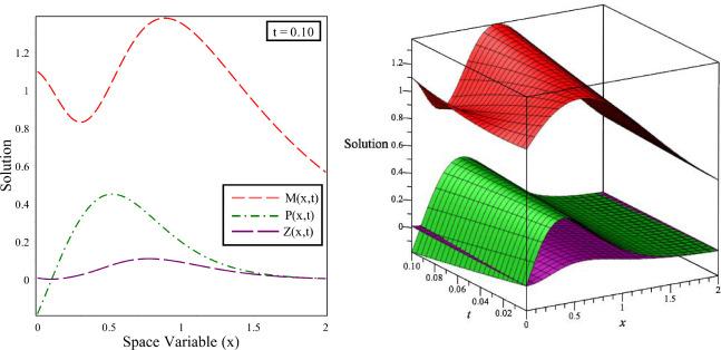
Fig.3 The solution behaviour of $M (x, t)$ , $P (x, t)$ , and $Z (x, t)$ versus distance in 2D and 3D for fixed time $t = 0.1$ and integer order $α = 1$ .

Fig. 4 shows the solution behaviour in 2D and 3D of east-west component of wind,

M (x, t)

versus distance

0 \leq x \leq 2

for different time

t

and integer-order

α = 1 .

Fig. 5, Fig. 6, Fig. 7 depict the physical behaviour of the solution of fractional-order atmospheric internal wave model for east-west component of wind (velocity)

(M (x, t))

, versus space variable

x

at different time

t = 0.02, 0.06, 0.10

, different fractional-order values

α = 0.7, 0.8, 0.9

and integer-order

α = 1

. It is clear from Fig. 4 that the waves become unstable when time increases.

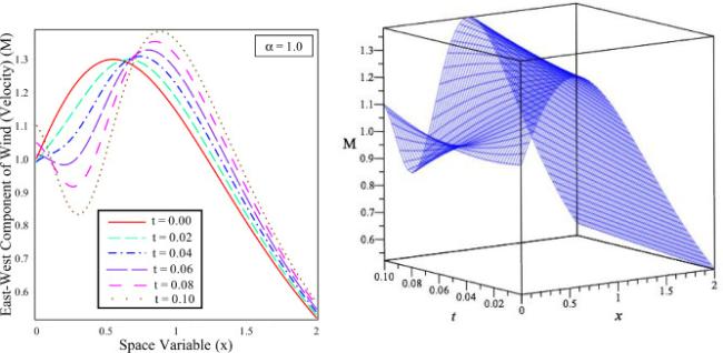
View original graphic|Download|PPT slide

Fig.4 The solution behaviour of East-West Component of wind (velocity) ( $M (x, t$ )) versus distance in 2D and 3D for different time $t$ .

View original graphic|Download|PPT slide

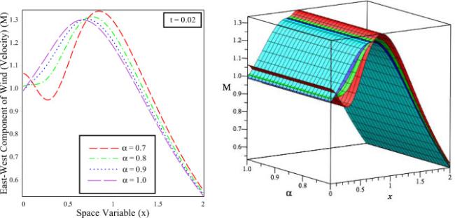
Fig.5 The solution behaviour of East-West Component of wind (velocity) ( $M (x, t$ )) versus distance in 2D and 3D for fixed time $t = 0.02$ different fractional order values $α = 0.7, 0.8, 0.9$ and integer order $α = 1$ .

View original graphic|Download|PPT slide

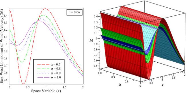
Fig.6 The solution behaviour of East-West Component of wind (velocity) ( $M (x, t$ )) versus distance in 2D and 3D for fixed time $t = 0.06$ different fractional order values $α = 0.7, 0.8, 0.9$ and integer order $α = 1$ .

View original graphic|Download|PPT slide

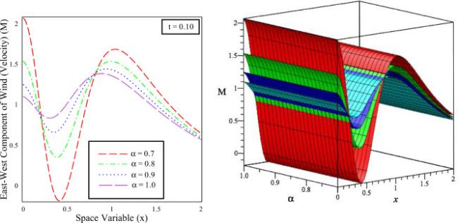
Fig.7 The solution behaviour of East-West Component of wind (velocity) ( $M (x, t$ )) versus distance in 2D and 3D for fixed time $t = 0.10$ different fractional order values $α = 0.7, 0.8, 0.9$ and integer order $α = 1$ .

Fig. 8 shows the solution behaviour in 2D and 3D of north-south component of wind (velocity)

(P (x, t))

versus distance

0 \leq x \leq 2

for different time

t

and integer-order

α = 1 .

Fig. 9, Fig. 10, Fig. 11 depict the physical behaviour of the solution of fractional-order atmospheric internal wave model for east-west component of wind (velocity)

(M (x, t))

, versus space variable

x

at different time

t = 0.02, 0.06, 0.10

, different fractional-order values

α = 0.7, 0.8, 0.9

and integer-order

α = 1

View original graphic|Download|PPT slide

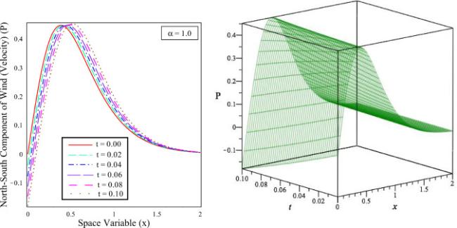
Fig.8 The solution behaviour of North-South Component of wind (velocity) ( $P (x, t)$ ) versus distance in 2D and 3D for different time.

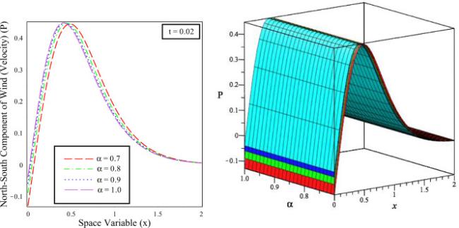
View original graphic|Download|PPT slide

Fig.9 The solution behaviour of North-South Component of wind (velocity) ( $P (x, t)$ ) versus distance in 2D and 3D for fixed time $t = 0.02$ different fractional order values $α = 0.7, 0.8, 0.9$ and integer order $α = 1$ .

View original graphic|Download|PPT slide

Fig.10 The solution behaviour of North-South Component of wind (velocity) ( $P (x, t)$ ) versus distance in 2D and 3D for fixed time $t = 0.06$ different fractional order values $α = 0.7, 0.8, 0.9$ and integer order $α = 1$ .

View original graphic|Download|PPT slide

Fig.11 The solution behaviour of North-South Component of wind (velocity) ( $P (x, t)$ ) versus distance in 2D and 3D for fixed time $t = 0.10$ different fractional order values $α = 0.7, 0.8, 0.9$ and integer order $α = 1$ .

Fig. 12 shows the solution behaviour in 2D and 3D of depth of a fluid,

(Z (x, t))

versus distance

0 \leq x \leq 2

for different time

t

and integer-order

α = 1 .

Fig. 13, Fig. 14, Fig. 15 depict the physical behaviour of the solution of fractional-order atmospheric internal wave model for east-west component of wind (velocity)

(M (x, t))

, versus space variable

x

at different time

t = 0.02, 0.06, 0.10

, different fractional-order values

α = 0.7, 0.8, 0.9

and integer-order

α = 1

. It can be observed from the Fig. 13, Fig. 14, Fig. 15 that when time increases the fluctuation in depth of fluid increases.

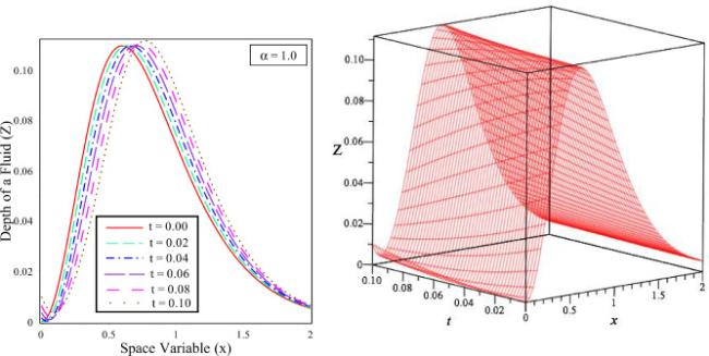
View original graphic|Download|PPT slide

Fig.12 The solution behaviour of depth of fluid versus ( $Z (x, t)$ ) distance ( $x$ ) in 2D and 3D for different time $t$ .

View original graphic|Download|PPT slide

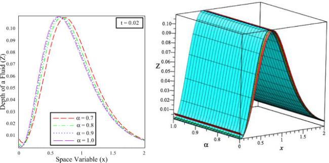
Fig.13 The solution behaviour of depth of fluid versus ( $Z (x, t)$ ) distance ( $x$ ) in 2D and 3D for fixed time $t = 0.02$ different fractional order values $α = 0.7, 0.8, 0.9$ and integer order $α = 1$ .

View original graphic|Download|PPT slide

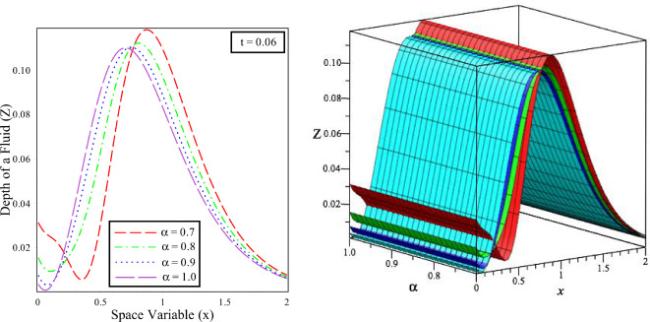
Fig.14 The solution behaviour of depth of fluid ( $Z (x, t)$ ) versus distance ( $x$ ) in 2D and 3D for fixed time $t = 0.06$ different fractional order values $α = 0.7, 0.8, 0.9$ and integer order $α = 1$ .

View original graphic|Download|PPT slide

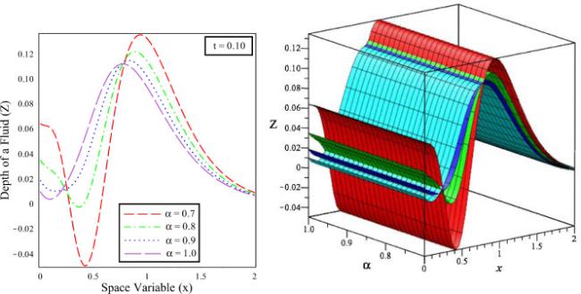
Fig.15 The solution behaviour of depth of fluid ( $Z (x, t)$ ) versus distance ( $x$ ) in 2D and 3D for fixed time $t = 0.10$ different fractional order values $α = 0.7, 0.8, 0.9$ and integer order $α = 1$ .

Tables 1, 2 and 3 show numerical comparison between FRDTM, EADM [10], HAM [8] and numerical solution for integer-order

α = 1

. The obtained results prove that the FRDTM gives fast convergence of the solutions without using Adomian polynomials, discretization, transformation, shape parameters, restrictive assumptions, or linearization for solving for nonlinear time-fractional differential equations. The method can also be easily extended to similar equations that arise in real-world problems.

Table 1 Numerical comparison of $M (x, t)$ for different spaces and times.

x	t=0				t=0.02				t=0.04
Empty Cell	FRDTM	EADM [10]	HAM [8]	NUM	FRDTM	EADM [10]	HAM [8]	NUM	FRDTM	EADM [10]	HAM [8]	NUM
0.0	1.00000	1.00000	1.00000	1.00000	0.98766	0.98000	0.98350	0.97226	0.98911	0.96000	0.96700	0.98792
0.2	1.17382	1.17382	1.17382	1.17382	1.10403	1.10026	1.11313	1.10934	1.04412	1.02669	1.05244	1.05275
0.4	1.27646	1.27646	1.27646	1.27646	1.22231	1.22755	1.23611	1.21777	1.15984	1.17863	1.19575	1.15837
0.6	1.29658	1.29658	1.29658	1.29658	1.29335	1.29910	1.29866	1.28681	1.27748	1.30162	1.30074	1.27049
0.8	1.24420	1.24420	1.24420	1.24420	1.27483	1.27677	1.27107	1.27570	1.30042	1.30933	1.29793	1.29907
1.0	1.14161	1.14161	1.14161	1.14161	1.18152	1.18095	1.17406	1.18742	1.22226	1.22029	1.20652	1.22837
1.2	1.01270	1.01270	1.01270	1.01270	1.04835	1.04712	1.04110	1.05252	1.08655	1.08154	1.06949	1.09214
1.4	0.87654	0.87654	0.87654	0.87654	0.90377	0.90272	0.89814	0.90394	0.93323	0.92890	0.91974	0.93390
1.6	0.74557	0.74557	0.74557	0.74557	0.76473	0.76404	0.76081	0.76325	0.78537	0.78251	0.77604	0.78358
1.8	0.62649	0.62649	0.62649	0.62649	0.63937	0.63897	0.63678	0.63835	0.65310	0.65144	0.64707	0.65179
2.0	0.52204	0.52204	0.52204	0.52204	0.53047	0.53025	0.52882	0.53005	0.53936	0.53846	0.53559	0.53882

Table 2 Numerical comparison of $P (x, t)$ for different spaces and times.

x	t=0				t=0.02				t=0.04
Empty Cell	FRDTM	EADM [10]	HAM [8]	NUM	FRDTM	EADM [10]	HAM [8]	NUM	FRDTM	EADM [10]	HAM [8]	NUM
0.0	0.00000	0.00000	0.00000	0.00000	-	-	-	-	-	-	-
					0.03930	0.04000	0.03300	0.03954	0.07760	0.07999	0.06599	0.07829
0.2	0.34226	0.34226	0.34226	0.34226	0.31364	0.31430	0.31919	0.31182	0.28422	0.28634	0.29612	0.28101
0.4	0.44724	0.44724	0.44724	0.44724	0.44744	0.44903	0.44872	0.44536	0.44446	0.45082	0.45019	0.44185
0.6	0.36602	0.36602	0.36602	0.36602	0.38151	0.38186	0.37909	0.38176	0.39599	0.39769	0.39215	0.39581
0.8	0.24084	0.24084	0.24084	0.24084	0.25593	0.25545	0.25290	0.25719	0.27191	0.27006	0.26495	0.27324
1.0	0.14130	0.14130	0.14130	0.14130	0.15099	0.15052	0.14891	0.15133	0.16169	0.15974	0.15652	0.16213
1.2	0.07772	0.07772	0.07772	0.07772	0.08287	0.08261	0.08175	0.08247	0.08860	0.08749	0.08579	0.08810
1.4	0.04111	0.04111	0.04111	0.04111	0.04358	0.04346	0.04305	0.04319	0.04631	0.04581	0.04499	0.04578
1.6	0.02120	0.02120	0.02120	0.02120	0.02231	0.02226	0.02208	0.02214	0.02353	0.02333	0.02296	0.02329
1.8	0.01073	0.01073	0.01073	0.01073	0.01122	0.01120	0.01112	0.01117	0.01174	0.01167	0.01151	0.01167
2.0	0.00536	0.00536	0.00536	0.00536	0.00557	0.00556	0.00553	0.00556	0.00579	0.00577	0.00570	0.00577

Table 3 Numerical comparison of $Z (x, t)$ for different spaces and times.

x	t=0				t=0.02				t=0.04
Empty Cell	FRDTM	EADM [10]	HAM [8]	NUM	FRDTM	EADM [10]	HAM [8]	NUM	FRDTM	EADM [10]	HAM [8]	NUM
0.0	0.00000	0.00000	0.00000	0.00000	0.00000	0.00000	0.00000	0.00000	0.00000	0.00000	0.00000	0.00000
0.2	0.03423	0.03423	0.03423	0.03423	0.02745	0.02693	0.02820	0.02769	0.02180	0.01963	0.02218	0.02185
0.4	0.08945	0.08945	0.08945	0.08945	0.08317	0.08355	0.08458	0.08243	0.07642	0.07765	0.07971	0.07580
0.6	0.10981	0.10981	0.10981	0.10981	0.10940	0.11002	0.10998	0.10833	0.10764	0.11024	0.11016	0.10638
0.8	0.09634	0.09634	0.09634	0.09634	0.09981	0.09997	0.09933	0.09992	0.10285	0.10360	0.10233	0.10269
1.0	0.07065	0.07065	0.07065	0.07065	0.07460	0.07449	0.07382	0.07529	0.07877	0.07833	0.07698	0.07954
1.2	0.04663	0.04663	0.04663	0.04663	0.04954	0.04941	0.04892	0.04984	0.05275	0.05218	0.05121	0.05317
1.4	0.02878	0.02878	0.02878	0.02878	0.03054	0.03045	0.03016	0.03043	0.03249	0.03212	0.03154	0.03236
1.6	0.01696	0.01696	0.01696	0.01696	0.01791	0.01786	0.01770	0.01775	0.01895	0.01877	0.01845	0.01875
1.8	0.00966	0.00966	0.00966	0.00966	0.01014	0.01012	0.01004	0.01007	0.01066	0.01058	0.01042	0.01057
2.0	0.00536	0.00536	0.00536	0.00536	0.00559	0.00558	0.00555	0.00557	0.00584	0.00580	0.00573	0.00581

6. Conclusion

In this study, FRDTM is the efficient mathematical tool applied to find an approximate solution of the atmospheric internal waves model which provides a realistic portrayal of the phenomenon. Fig. 3, Fig. 4, Fig. 5, Fig. 6, Fig. 7, Fig. 8, Fig. 9, Fig. 10, Fig. 11, Fig. 12, Fig. 13, Fig. 14, Fig. 15 portray that FRDTM can tackle the problems perfectly and it can be deployed in ocean engineering for analyzing water waves with linear and non-linear nature. Finally, the fractional solution provides a pragmatic look into the physical behaviour of internal waves which can be helpful to refine climate and weather models as the waves have a significant influence on climate change.

Declaration of Competing Interest

The authors declare that they have no known competingfinancial interests or personal relationships that could have appeared toinfluence the work reported in this paper.

References

Publishing order | Descend order by publishing year | Descend order by cited within

[1]	S. Chakrabarti. Handbook of Offshore Engineering (2-Volume Set). Elsevier (2005)

[2]	D.Y. Le Roux, A. Staniforth, C.A. Lin. Mon. Weather Rev., 126 (7) (1998), pp. 1931-1951

[3]	D. Aguilar,B. Sutherland. Phys. Fluids, 18 (6) (2006), p. 066603

[4]	J.P. Boyd, C. Zhou. J. Fluid Mech., 617 (2008), pp. 187-205

[5]	A. Imani, D. Ganji, H.B. Rokni, H. Latifizadeh, E. Hesameddini, M.H. Rafiee. Appl. Math. Model., 36 (4) (2012), pp. 1550-1557

[6]	P. Karunakar, S. Chakraverty. Int. J. Numer. Methods Heat Fluid Flow, 27 (9) (2017), pp. 2015-2029

[7]	H. Hermansyah, et al.. J. Appl. Math., 2018 ( 2018), pp. 1-5, DOI: 6835179

[8]	Z. Busrah, T. Bakhtiar, et al.. IOSR J. Math., 10 (5) ( 2014), pp. 46-53 DOI: 10.9790/5728-10554653

[9]	A.C. Varsoliwala, T.R. Singh. J. Ocean Eng. Sci., 6 (4) (2021), pp. 367-375, DOI: https://www.sciencedirect.com/science/article/pii/S2468013321000255/pdfft?md5=b7a0a443c39c2f1036b4cd7b73479fc1&pid=1-s2.0-S2468013321000255-main.pdf

[10]	A.C. Varsoliwala, T.R. Singh. J. Ocean Eng. Sci. (2021), DOI: In press

[11]	T. Patel, R. Meher. Nonlinear Eng., 6 (3) (2017), pp. 191-200

[12]	T. Patel,R. Meher. Nonlinear Eng., 8 (1) (2019), pp. 145-156 DOI: 10.1515/nleng-2017-0135

[13]	A. Goswami, J. Singh, D. Kumar, S. Gupta, et al.. J. Ocean Eng. Sci., 4 (2) (2019), pp. 85-99

[14]	V. Moradi, K. Sayevand. Math. Methods Appl. Sci., 44 (15) (2020), pp. 11944-11960

[15]	P. Tandel, H. Patel, T. Patel. J. Ocean Eng. Sci. (2021), DOI: In press

[16]	V.K. Tamboli, P.V. Tandel. J. Ocean Eng. Sci. (2021), DOI: In press

[17]	I. Dassios,F. Font. Math. Methods Appl. Sci., 44 (15) (2021), pp. 11844-11855 DOI: 10.1002/mma.6506

[18]	T.T. Warner.Numerical Weather and Climate Prediction. Cambridge University Press (2010)

[19]	Y. Keskin, G. Oturanc. Int. J. Nonlinear Sci. Numer. Simul., 10 (6) (2009), pp. 741-750

[20]	H.S. Patel, T. Patel. Int. J. Appl. Comput. Math., 7 (5) (2021), pp. 1-15

[21]	S.R. Moosavi Noori, N. Taghizadeh. Int. J. Differ. Equ.,2021 (2021), pp. 1-16, DOI: 6696414

Options

Abstract

Outlines

模态框（Modal）标题

Abstract

Cite this article

1. Introduction

Fig.1 Internal waves in (a) south china sea (STS-7, June 1983, picture-#7-05-0245) and (b) Eastern Pacific Sea (STS-41C, April 1984, picture-#13-31-980).

Fig.2 Schematic representation of internal waves.

2. Mathematical model formulation

3. Formulation of fractional reduced differential transform method

4. Application of FRDTM

5. Results and discussion

Fig.3 The solution behaviour of M(x,t), P(x,t), and Z(x,t) versus distance in 2D and 3D for fixed time t=0.1 and integer order α=1.

Fig.4 The solution behaviour of East-West Component of wind (velocity) (M(x,t)) versus distance in 2D and 3D for different time t.

Fig.5 The solution behaviour of East-West Component of wind (velocity) (M(x,t)) versus distance in 2D and 3D for fixed time t=0.02 different fractional order values α=0.7,0.8,0.9 and integer order α=1.

Fig.6 The solution behaviour of East-West Component of wind (velocity) (M(x,t)) versus distance in 2D and 3D for fixed time t=0.06 different fractional order values α=0.7,0.8,0.9 and integer order α=1.

Fig.7 The solution behaviour of East-West Component of wind (velocity) (M(x,t)) versus distance in 2D and 3D for fixed time t=0.10 different fractional order values α=0.7,0.8,0.9 and integer order α=1.

Fig.8 The solution behaviour of North-South Component of wind (velocity) (P(x,t)) versus distance in 2D and 3D for different time.

Fig.9 The solution behaviour of North-South Component of wind (velocity) (P(x,t)) versus distance in 2D and 3D for fixed time t=0.02 different fractional order values α=0.7,0.8,0.9 and integer order α=1.

Fig.10 The solution behaviour of North-South Component of wind (velocity) (P(x,t)) versus distance in 2D and 3D for fixed time t=0.06 different fractional order values α=0.7,0.8,0.9 and integer order α=1.

Fig.11 The solution behaviour of North-South Component of wind (velocity) (P(x,t)) versus distance in 2D and 3D for fixed time t=0.10 different fractional order values α=0.7,0.8,0.9 and integer order α=1.

Fig.12 The solution behaviour of depth of fluid versus (Z(x,t)) distance (x) in 2D and 3D for different time t.

Fig.13 The solution behaviour of depth of fluid versus (Z(x,t)) distance (x) in 2D and 3D for fixed time t=0.02 different fractional order values α=0.7,0.8,0.9 and integer order α=1.

Fig.14 The solution behaviour of depth of fluid (Z(x,t)) versus distance (x) in 2D and 3D for fixed time t=0.06 different fractional order values α=0.7,0.8,0.9 and integer order α=1.

Fig.15 The solution behaviour of depth of fluid (Z(x,t)) versus distance (x) in 2D and 3D for fixed time t=0.10 different fractional order values α=0.7,0.8,0.9 and integer order α=1.

Table 1 Numerical comparison of M(x,t)for different spaces and times.

Table 2 Numerical comparison of P(x,t) for different spaces and times.

Table 3 Numerical comparison of Z(x,t) for different spaces and times.

6. Conclusion

Declaration of Competing Interest

References

Links

Fig.3 The solution behaviour of $M (x, t)$ , $P (x, t)$ , and $Z (x, t)$ versus distance in 2D and 3D for fixed time $t = 0.1$ and integer order $α = 1$ .

Fig.4 The solution behaviour of East-West Component of wind (velocity) ( $M (x, t$ )) versus distance in 2D and 3D for different time $t$ .

Fig.5 The solution behaviour of East-West Component of wind (velocity) ( $M (x, t$ )) versus distance in 2D and 3D for fixed time $t = 0.02$ different fractional order values $α = 0.7, 0.8, 0.9$ and integer order $α = 1$ .

Fig.6 The solution behaviour of East-West Component of wind (velocity) ( $M (x, t$ )) versus distance in 2D and 3D for fixed time $t = 0.06$ different fractional order values $α = 0.7, 0.8, 0.9$ and integer order $α = 1$ .

Fig.7 The solution behaviour of East-West Component of wind (velocity) ( $M (x, t$ )) versus distance in 2D and 3D for fixed time $t = 0.10$ different fractional order values $α = 0.7, 0.8, 0.9$ and integer order $α = 1$ .

Fig.8 The solution behaviour of North-South Component of wind (velocity) ( $P (x, t)$ ) versus distance in 2D and 3D for different time.

Fig.9 The solution behaviour of North-South Component of wind (velocity) ( $P (x, t)$ ) versus distance in 2D and 3D for fixed time $t = 0.02$ different fractional order values $α = 0.7, 0.8, 0.9$ and integer order $α = 1$ .

Fig.10 The solution behaviour of North-South Component of wind (velocity) ( $P (x, t)$ ) versus distance in 2D and 3D for fixed time $t = 0.06$ different fractional order values $α = 0.7, 0.8, 0.9$ and integer order $α = 1$ .

Fig.11 The solution behaviour of North-South Component of wind (velocity) ( $P (x, t)$ ) versus distance in 2D and 3D for fixed time $t = 0.10$ different fractional order values $α = 0.7, 0.8, 0.9$ and integer order $α = 1$ .

Fig.12 The solution behaviour of depth of fluid versus ( $Z (x, t)$ ) distance ( $x$ ) in 2D and 3D for different time $t$ .

Fig.13 The solution behaviour of depth of fluid versus ( $Z (x, t)$ ) distance ( $x$ ) in 2D and 3D for fixed time $t = 0.02$ different fractional order values $α = 0.7, 0.8, 0.9$ and integer order $α = 1$ .

Fig.14 The solution behaviour of depth of fluid ( $Z (x, t)$ ) versus distance ( $x$ ) in 2D and 3D for fixed time $t = 0.06$ different fractional order values $α = 0.7, 0.8, 0.9$ and integer order $α = 1$ .

Fig.15 The solution behaviour of depth of fluid ( $Z (x, t)$ ) versus distance ( $x$ ) in 2D and 3D for fixed time $t = 0.10$ different fractional order values $α = 0.7, 0.8, 0.9$ and integer order $α = 1$ .

Table 1 Numerical comparison of $M (x, t)$ for different spaces and times.

Table 2 Numerical comparison of $P (x, t)$ for different spaces and times.

Table 3 Numerical comparison of $Z (x, t)$ for different spaces and times.