New-fashioned solitons of coupled nonlinear Maccari systems describing the motion of solitary waves in fluid flow

Tarikul Islam; Ali Akbar; Hadi Rezazadeh; Ahmet Bekir

doi:10.1016/j.joes.2022.03.003

Journal of Ocean Engineering and Science >

2024 , Vol. 9 >Issue 4: 353 - 363

DOI: https://doi.org/10.1016/j.joes.2022.03.003

Original article

New-fashioned solitons of coupled nonlinear Maccari systems describing the motion of solitary waves in fluid flow

Tarikul Islam ^a ,
Ali Akbar ^b ,
Hadi Rezazadeh ^c ,
Ahmet Bekir ^,^d

Expand

^a Department of Mathematics, Hajee Mohammad Danesh Science and Technology University, Dinajpur, Bangladesh
^b Department of Applied Mathematics, University of Rajshahi, Bangladesh
^c Faculty of Modern Technologies Engineering, Amol University of Special Modern Technologies, Amol, Iran
^d Neighbourhood of Akcaglan, Imarli Street, No. 28/4, Eskisehir 26030, Turkey

Received date: 2021-08-19

Revised date: 2022-03-05

Accepted date: 2022-03-06

Online published: 2022-03-08

Fold

Abstract

The Schrodinger equation type nonlinear coupled Maccari system is a significant equation that flourished with the wide-ranging arena concerning fluid flow and the theory of deep-water waves, physics of plasma, nonlinear optics, etc. We exploit the enhanced tanh approach and the rational (Gâ€²/G) -expansion process to retrieve the soliton and dissimilar soliton solutions to the Maccari system in this study. The suggested systems of nonlinear equations turn into a differential equation of single variable through executing some operations of wave variable alteration. Thereupon, with the successful implementation of the advised techniques, a lot of exact soliton solutions are regained. The obtained solutions are depicted in 2D, 3D, and contour traces by assigning appropriate values of the allied unknown constants. These diverse graphical appearances assist the researchers to understand the underlying processes of intricate phenomena of the leading equations. The individual performances of the employed methods are praiseworthy which justify further application to unravel many other nonlinear evolution equations ascending in various branches of science and engineering.

Highlights

● We have obtained new solitons for the coupled nonlinear Maccari's system describing the motion of isolated waves in fluid-flow.

● This model describes propagation of solitons in the theory of deep-water waves.

● Abundant closed form wave solutions are successfully generated in terms of rational, trigonometric and hyperbolic functions.

● The acquired solutions alongside particular values of involved free parameters are figured out in 3D, 2D and contour profiles to depict diverse soliton patterns.

Key words： Rational ( $G^{'} / G$ )-expansion method; Coupled nonlinear schrodinger equations; Soliton; Improved tanh method; Exact solutions

Cite this article

Tarikul Islam , Ali Akbar , Hadi Rezazadeh , Ahmet Bekir . New-fashioned solitons of coupled nonlinear Maccari systems describing the motion of solitary waves in fluid flow[J]. Journal of Ocean Engineering and Science, 2024 , 9(4) : 353 -363 . DOI: 10.1016/j.joes.2022.03.003

1. Introduction

Nonlinear fractional and classical differential equations are significant tools to model and depict the interior behavior of complicated physical phenomena arise throughout the natural world [1], [2], [3]. That is why the researchers have paid attention to explore the analytical and numerical solutions of these equations [4], [5], [6], [7]. The continued efforts of scholars to examine the results of nonlinear partial differential equations attained through diverse approaches are opening new doors of research [8], [9], [10], [11], [12], [13], [14], [15], [16], [17], [18], [19], [20], [21].

The nonlinear Maccari system [30], [31], [32] is the Schrodinger equation type coupled equations

i q_{t} + q_{x x} + r q = 0,

i s_{t} + s_{x x} + r s = 0,

i n_{t} + n_{x x} + r n = 0,

(1.1)

r_{t} + r_{y} + {({| q + s + n |}^{2})}_{x} = 0,

where

q, s, n

stand for complex scalar fields,

r

represents real scalar fields and all depends on space-variables

x

y

and time-variable

t

, has wide-spectral applications in the theory of deep-water waves, fluid flow, plasma physics, nonlinear optics, etc. This system has been investigated by some researchers to unravel for exact wave solutions, such as Ciancio et al [22]. utilized the modified

exp (- ϕ (η))

-expansion function procedure to find solutions relating to hyperbolic and trigonometric functions; Inc et al [23]. studied this system by the use of the generalized Riccati equation scheme and modified F-expansion method; Neirameh employed the improved

(G^{'} / G)

-expansion scheme to acquire certain closed-from wave solutions [24]; Baskonus et al [25]. the Maccari system (1.1) by means of sine-Gordon expansion technique and found only hyperbolic type solutions; the modified trial equation process has been adopted by Bulut et al [26]. which provide few traveling wave solutions; Rostamy and Zabihi [27] have applied the first integral method to construct exponential functions and hyperbolic functions wave solutions. Vahidi et al [28]. studied the Maccari system by means of rational sinh-cosh and extended rational sine-cosine techniques, which is closely related to Eq. (1.1); Akbar et al [29]. have also considered the same system to extract by a generalized auxiliary equation mapping algorithm. Now, we have a brief look at the literature to recall the original foundation of Maccari system. This system containing two nonlinear evolution equations (Maccari, [30]) stands out among the nonlinear models for understanding the movement of solitary waves in plasmas, nonlinear optics, quantum field theory. Several studies relating to this system is available in the literature for instance Jabbari et al [31]. used

(G^{'} / G)

-expansion and He's semi-inverse techniques which provide estimations in terms rational, trigonometric and hyperbolic form; Khater et al [32]. studied the system by using general exp-function approach and obtained standard soliton solutions; Cheemaa et al [33]. used a modified auxiliary equation approach and found different types closed-form solutions; Liu et al [34]. have studied the same system and obtained bright and dark N-soliton solutions, Hafez et al [35]. examined this system through the new

(G^{'} / G)

-expansion scheme.

Khater et al [36]. analyzed the nonlinear Kolmogorov-Petrovskii-Piskunov model of fractional order by the use of the Adomian decomposition procedure and numerical approach. Chu et al [37]. investigated the general (2 + 1)-dimensional wave model arise in shallow-water using the simplest calculation approach and the advanced Kudryashov scheme. Khater et al [38]. studied the semi-analytical and analytical solutions to the fractional HIV-1 infection of CD4+ T -cells, and also approximate wave solutions to the complex nonlinear Fokas-Lenells models [39] of short pulses in optical fibers, the semi-exact estimations of the nonlinear Phi-4 equation [40], the numerical simulation of the time-space fractional telegraphic nonlinear equation [41]. Khater and Ghanbari [42] investigated the soliton solutions to the Chaffee-Infante model using five techniques. Khater et al [43]. scrutinized numerical estimations to the modified BBM model and examined the stability property of the attained solutions, abundant novel soliton solutions to the Klein-Fock-Gordon equation [44], the analytical solutions to the perturbed Schrödinger nonlinear equation [45], the analytical and semi-exact estimations to the time-fractional Cahn-Allen model [46], the numerical estimations to the Klein-Gordon-Zakharov equation [47], the analytical accurate traveling wave solutions of the higher-dimensional Schrödinger nonlinear model [48], the semi-analytical and exact estimation to the fractional quadratic-cubic Schrödinger equation [49]. Khater [50] unraveled abundant breather solutions to the Vakhnenko-Parkes equation by means of a couple of analytical approaches. Khater et al [51]. investigated the numerical solutions of two bio-mathematical and statistical fractional order nonlinear equations. Khater and Lu [52] searched numerical and exact solutions to the space and time fractional nonlinear telegraphic model using the trigonometric-quantic-B-spline method. Khater and Ahmed [53] evaluated the solutions of the Klein-Gordon-Zakharov nonlinear model by exponential cubic B-spline schemes. Khater et al [54]. derived bright-dark soliton to the (1 + 1)-dimensional nonlinear Kaup-Kupershmidt model utilizing modified F-expansion approach. Yue et al [55]. perused analytical estimations to the fractional Hirota-Satsuma models via the modified Kudryashov and the enhanced simplest equation tools. Li et al [56]. probed numerical estimations to the (2 + 1)-dimensional KPBBM model by employing the modified direct algebraic method. Khater and Alabdali [57] studied numerical and analytical wave solutions of (2 + 1)-dimensional Fisher-KolmogorovPetrovskii-Piskunov model by imposing the modified Kudryashov, trigonometric-quantic B-spline, and modified direct algebraic schemes.

To the furthest of our sagaciousness, the Maccari system (1.1) has not been studied using the enhanced tanh approach and the method of rational

(G^{'} / G)

-expansion. In continuation of the above works fascinate us and thereupon we aim to extract some primal and standard soliton solutions to the Maccari system through the indicated methods from which a number of reputed solutions will be re-established as well as some effective and reliable solitary solutions will be extracted. The closed waveform solutions are received in hyperbolic, rational, and trigonometric types. The well-furnished solutions are interpreted in 2D, 3D, and contour traces to bring out their physical meanings. It is designated that this work is new in the literature, and the results might have a substantial impact on ocean engineering [22], [23], [24], [25], [26], [27]. The Journal of Ocean Engineering and Science has published some results of various investigations [58], [59], [60], [61], [62], [63], [64] that are compatible with our findings. The considered governing model is concerned with the phenomena of water waves, fluid flow, plasma physics etc. which are related to wave energy converters and hence oceanography.

2. Explanation of the methods

A nonlinear evolution equation is assumed as

(2.1)

Θ (u, u_{x}, u_{y}, u_{t}, u_{x y}, u_{x t}, u_{y t}, u_{x x}, u_{y y}, u_{t t}, \dots) = 0,

where

Θ

consists of

u

and it distinct derivatives. The new wave variable adaptation

(2.2)

u = u (ϕ), ϕ = ϕ (x, y, t, \dots)

makes this equation to the following general differential equation relating to

ϕ

(2.3)

Λ (U, U^{'}, U^{″}, U^{″'}, \dots \dots \dots) = 0 .

As many times as feasible, we take the anti-derivative of Eq. (2.3). We can ignore the integral constant, since we are scrutinizing soliton solutions. The following are the key steps of the introduced techniques:

2.1. The improved tanh method

We estimate the solution of Eq. (2.3) in accordance with the improved tanh approach in the ensuing form

(2.1.1)

Q (ϕ) = \frac{ι_{0} + \sum_{i = 1}^{e} (ι_{i} Φ^{i} (ϕ) + τ_{i} Φ^{- i} (ϕ))}{\in_{0} + \sum_{i = 1}^{e} (\in_{i} Φ^{i} (ϕ) + ε_{i} Φ^{- i} (ϕ))}

whose unknown parameters are evaluated hereafter [65]. The integral value of

e

is set in view of the balancing principle applying to Eq. (2.3). The Riccati equation satisfying by

Φ = Φ (ϕ)

(2.1.2)

Φ^{'} (ϕ) = δ + Φ^{2} (ϕ),

where

δ

is a real arbitrary number Eq. (2.1.2). has the subsequent outcomes:

(2.1.3)

\begin{matrix} Φ (ϕ) & = & - \sqrt{- δ} tanh (\sqrt{- δ} ϕ) o r Φ (ϕ) \\ = & - \sqrt{- δ} coth (\sqrt{- δ} ϕ), δ < 0 \end{matrix}

(2.1.4)

Φ (ϕ) = - 1 / ϕ o r δ = 0

(2.1.5)

Φ (ϕ) = \sqrt{δ} tan (\sqrt{δ} ϕ) o r Φ (ϕ) = - \sqrt{δ} cot (\sqrt{δ} ϕ), δ > 0

When Eq. (2.3) is combined with Eqs. (2.1.1) and (2.1.2), a polynomial in

Φ (ϕ)

is obtained. We unravel the equations using computational software that equalizes the coefficients of this polynomial to zero for the values of the arbitrary numbers belonging to Eq. (2.1.1). We substitute the received values in Eq. (2.1.1), which, when combined with the solutions of Eq. (2.1.2), result the exact traveling wave solutions of Eq. (2.1).

2.2. The rational $(G^{'} / G)$ -expansion method

In the following form,

(2.2.1)

Q (ϕ) = \frac{\sum_{i = 0}^{e} ι_{i} {(G^{'} (ϕ) / G (ϕ))}^{i}}{\sum_{i = 0}^{e} τ_{i} {(G^{'} (ϕ) / G (ϕ))}^{i}},

we estimate the solution of Eq. (2.3) using the enhanced tanh technique, where

e

is determined by equilibrium state the linear and nonlinear terms of the maximum order appearing in Eq. (2.3) and unknown constants

{a_{i}}^{'} s

and

{b_{i}}^{'} s

are calculated after some operations [66]. The function

G (ϕ)

satisfies

(2.2.2)

G^{″} (ϕ) + b G^{'} (ϕ) + c G (ϕ) = 0

This ODE leaves,

(2.2.3)

\frac{G^{'} (ϕ)}{G (ϕ)} = - b + \sqrt{b^{2} - 4 c} \tanh (0.5 \sqrt{b^{2} - 4 c} ϕ) / 2, b^{2} - 4 c > 0

(2.2.4)

\frac{G^{'} (ϕ)}{G (ϕ)} = {- b + \sqrt{b^{2} - 4 c} \coth (0.5 \sqrt{b^{2} - 4 c} ϕ)} / 2, b^{2} - 4 c > 0

(2.2.5)

\frac{G^{'} (ϕ)}{G (ϕ)} = \frac{1}{ϕ} - \frac{b}{2}, b^{2} - 4 c = 0

(2.2.6)

\frac{G^{'} (ϕ)}{G (ϕ)} = {- b - \sqrt{4 c - b^{2}} \tan (0.5 \sqrt{4 c - b^{2}} ϕ)} / 2, b^{2} - 4 c < 0

(2.2.7)

\frac{G^{'} (ϕ)}{G (ϕ)} = {- b + \sqrt{4 c - b^{2}} \cot (0.5 \sqrt{4 c - b^{2}} ϕ)} / 2, b^{2} - 4 c < 0

With the help of Eqs. (2.2.1) and (2.2.2), from Eq. (2.3) it is resulted a polynomial in

(G^{'} (ϕ) / G (ϕ))

with zero coefficients, yielding a set of algebraic equations. We use Maple to unravel the system and seek for the values of the arbitrary numbers occur in Eq. (2.2.1). The accurate traveling wave solutions of Eq. (2.1) are then obtained by combining these values into solution (2.2.1).

3. Formulation of solutions

In this part, the nonlinear coupled Maccari system is considered to be unraveled by means of two competent tools like the approach of rational

(G^{'} / G)

-expansion and improved tanh function method. We introduce the transformation,

q (x, y, t) = Q (ϕ) e^{i ψ}, s (x, y, t) = S (ϕ) e^{i ψ}

(3.1)

n (x, y, t) = N (ϕ) e^{i ψ}, r (x, y, t) = R (ϕ)

where

ϕ = x + y - 2 κ t

ψ = κ x + α y + γ t + ζ

After specific operation on Eq. (1.1) by the support of Eq. (3.1) turns into the resulting equation:

(3.2)

(1 - 2 κ) Q^{″} - (1 - 2 κ) (γ + κ^{2}) Q - {(1 + λ + μ)}^{2} Q^{3} = 0,

where

S = λ Q

N = μ Q

and

R = \frac{{(1 + λ + μ)}^{2} Q^{2}}{2 κ - 1}

Balancing the terms

Q^{″}

and

Q^{3}

we determine

e = 1

. Thereupon, the advised techniques are adopted to seek for solitary wave solutions of Eq. (1.1) in appropriate form.

3.1. The improved tanh method

(3.1.1)

Q (ϕ) = \frac{ι_{0} + ι_{1} Φ (ϕ) + τ_{1} Φ^{- 1} (ϕ)}{\in_{0} + \in_{1} Φ (ϕ) + ε_{1} Φ^{- 1} (ϕ)}

By the assistance of solution (3.1.1) and wave transformation (2.1.1), Eq. (3.2) becomes a polynomial in

Φ (ϕ)

. By setting zero to all coefficients of this polynomial and solving those with the computer package, we get the results

Set 1:

(3.1.2)

ι_{0} = ι_{1} = 0, \in_{0} = \pm \frac{2 τ_{1} (1 + λ + μ)}{(γ + κ^{2}) \sqrt{2 - 4 κ}}, \in_{1} = ε_{1} = 0, δ = \frac{γ + κ^{2}}{2}

Set 2:

(3.1.3)

ι_{0} = 0, τ_{1} = - \frac{ι_{1} (γ + κ^{2})}{4}, \in_{0} = \pm \frac{ι_{1} (1 + λ + μ)}{\sqrt{2 - 4 κ}}, \in_{1} = 0, δ = - \frac{γ + κ^{2}}{4}

Set 3:

(3.1.4)

\begin{matrix} ι_{0} = \pm \frac{ε_{1} \sqrt{2 - 4 κ}}{1 + λ + μ}, ι_{1} = \in_{1} = 0, τ_{1} = \mp \frac{ε_{1} \sqrt{(2 - 4 κ) (2 γ + 2 κ^{2})}}{2 (1 + λ + μ)}, \\ \in_{0} = \frac{2 ε_{1}}{\sqrt{2 γ + 2 κ^{2}}}, δ = \frac{γ + κ^{2}}{2} \end{matrix}

Set 4:

(3.1.5)

\begin{matrix} ι_{0} = \pm \frac{ε_{1} \sqrt{2 - 4 κ}}{1 + λ + μ}, ι_{1} = 0, τ_{1} = \mp \frac{\in_{0} (γ + κ^{2}) \sqrt{(2 - 4 κ)}}{2 (1 + λ + μ)}, \\ \in_{1} = 0, δ = \frac{γ + κ^{2}}{2} \end{matrix}

Set 5:

(3.1.6)

\begin{matrix} ι_{0} = 0, τ_{1} = - \frac{ι_{1} (γ + κ^{2})}{8}, \in_{0} = \pm \frac{ι_{1} (1 + λ + μ)}{\sqrt{2 - 4 κ}}, \\ \in_{1} = 0, ε_{1} = 0, δ = \frac{γ + κ^{2}}{8} \end{matrix}

Set 6:

(3.1.7)

\begin{matrix} ι_{0} = \pm \frac{ε_{1} \sqrt{2 - 4 κ}}{1 + λ + μ}, τ_{1} = 0, \in_{0} = \pm \frac{ι_{1} (1 + λ + μ)}{\sqrt{2 - 4 κ}}, \\ \in_{1} = 0, δ = \frac{γ + κ^{2}}{2} \end{matrix}

Injecting the scores appeared in Eq. (3.1.2) into Eq. (3.1.1) and thereupon adopting Eqs. (2.1.3)-(2.1.5) provide the following solitary wave solutions:

For

δ < 0

, the solutions are received in hyperbolic function form as

(3.1.8)

q_{1} (x, y, t) = \frac{\pm (γ + κ^{2}) \sqrt{2 - 4 κ} e^{i ψ} coth (\sqrt{- δ} ϕ)}{2 τ_{1} \sqrt{- δ} (1 + λ + μ)},

(3.1.9)

q_{2} (x, y, t) = \frac{\pm (γ + κ^{2}) \sqrt{2 - 4 κ} e^{i ψ} tanh (\sqrt{- δ} ϕ)}{2 τ_{1} \sqrt{- δ} (1 + λ + μ)},

(3.1.10)

s_{1} (x, y, t) = \frac{\pm λ (γ + κ^{2}) \sqrt{2 - 4 κ} e^{i ψ} coth (\sqrt{- δ} ϕ)}{2 τ_{1} \sqrt{- δ} (1 + λ + μ)},

(3.1.11)

s_{2} (x, y, t) = \frac{\pm λ (γ + κ^{2}) \sqrt{2 - 4 κ} e^{i ψ} tanh (\sqrt{- δ} ϕ)}{2 τ_{1} \sqrt{- δ} (1 + λ + μ)},

(3.1.12)

n_{1} (x, y, t) = \frac{\pm μ (γ + κ^{2}) \sqrt{2 - 4 κ} e^{i ψ} coth (\sqrt{- δ} ϕ)}{2 τ_{1} \sqrt{- δ} (1 + λ + μ)},

(3.1.13)

n_{2} (x, y, t) = \frac{\pm μ (γ + κ^{2}) \sqrt{2 - 4 κ} e^{i ψ} tanh (\sqrt{- δ} ϕ)}{2 τ_{1} \sqrt{- δ} (1 + λ + μ)},

(3.1.14)

r_{1} (x, y, t) = \frac{{(γ + κ^{2})}^{2}}{2 τ_{1}^{2} δ} \coth^{2} (\sqrt{- δ} ϕ),

(3.1.15)

r_{2} (x, y, t) = \frac{{(γ + κ^{2})}^{2}}{2 τ_{1}^{2} δ} \tanh^{2} (\sqrt{- δ} ϕ),

where

ϕ = x + y - 2 κ t

and

ψ = κ x + α y + γ t + ζ

Under the assumption

δ = 0

the rational function solutions are

(3.1.16)

q_{3} (x, y, t) = \frac{\pm (γ + κ^{2}) \sqrt{2 - 4 κ} ϕ e^{i ψ}}{2 τ_{1} (1 + λ + μ)},

(3.1.17)

s_{3} (x, y, t) = \frac{\pm λ (γ + κ^{2}) \sqrt{2 - 4 κ} ϕ e^{i ψ}}{2 τ_{1} (1 + λ + μ)},

(3.1.18)

n_{3} (x, y, t) = \frac{\pm μ (γ + κ^{2}) \sqrt{2 - 4 κ} ϕ e^{i ψ}}{2 τ_{1} (1 + λ + μ)},

(3.1.19)

r_{3} (x, y, t) = - \frac{{(γ + κ^{2})}^{2} ϕ^{2}}{2 τ_{1}^{2}},

where

ϕ = x + y - 2 κ t

and

ψ = κ x + α y + γ t + ζ

For the postulate

δ > 0

the trigonometric solutions are appeared as

(3.1.20)

q_{4} (x, y, t) = \frac{\pm (γ + κ^{2}) \sqrt{2 - 4 κ} e^{i ψ} cot (\sqrt{δ} ϕ)}{2 τ_{1} \sqrt{δ} (1 + λ + μ)},

(3.1.21)

q_{5} (x, y, t) = \frac{\pm (γ + κ^{2}) \sqrt{2 - 4 κ} e^{i ψ} tan (\sqrt{δ} ϕ)}{2 τ_{1} \sqrt{δ} (1 + λ + μ)},

(3.1.22)

s_{4} (x, y, t) = \frac{\pm λ (γ + κ^{2}) \sqrt{2 - 4 κ} e^{i ψ} cot (\sqrt{δ} ϕ)}{2 τ_{1} \sqrt{δ} (1 + λ + μ)},

(3.1.23)

s_{5} (x, y, t) = \frac{\pm λ (γ + κ^{2}) \sqrt{2 - 4 κ} e^{i ψ} tan (\sqrt{δ} ϕ)}{2 τ_{1} \sqrt{δ} (1 + λ + μ)},

(3.1.24)

n_{4} (x, y, t) = \frac{\pm μ (γ + κ^{2}) \sqrt{2 - 4 κ} e^{i ψ} cot (\sqrt{δ} ϕ)}{2 τ_{1} \sqrt{δ} (1 + λ + μ)},

(3.1.25)

n_{5} (x, y, t) = \frac{\pm μ (γ + κ^{2}) \sqrt{2 - 4 κ} e^{i ψ} tan (\sqrt{δ} ϕ)}{2 τ_{1} \sqrt{δ} (1 + λ + μ)},

(3.1.26)

r_{4} (x, y, t) = - \frac{{(γ + κ^{2})}^{2} \cot^{2} (\sqrt{δ} ϕ)}{2 τ_{1}^{2} δ},

(3.1.27)

r_{5} (x, y, t) = - \frac{{(γ + κ^{2})}^{2} \tan^{2} (\sqrt{δ} ϕ)}{2 τ_{1}^{2} δ},

where

ϕ = x + y - 2 κ t

and

ψ = κ x + α y + γ t + ζ

Utilizing the values involved in Eq. (3.1.3) into Eq. (3.1.1) and then adopting Eqs. (2.1.3)-(2.1.5) deliver the closed form traveling wave solutions as bellow:

Considering

δ < 0

the subsequent hyperbolic form solutions are attained

(3.1.28)

\begin{matrix} q_{6} (x, y, t) = \frac{\pm \sqrt{2 - 4 κ} e^{i ψ}}{4 \sqrt{- δ} (1 + λ + μ)} \times \\ {4 δ tanh (\sqrt{- δ} ϕ) + (γ + κ^{2}) coth (\sqrt{- δ} ϕ)}, \end{matrix}

(3.1.29)

\begin{matrix} q_{7} (x, y, t) = \frac{\pm \sqrt{2 - 4 κ} e^{i ψ}}{4 \sqrt{- δ} (1 + λ + μ)} \times \\ {4 δ coth (\sqrt{- δ} ϕ) + (γ + κ^{2}) tanh (\sqrt{- δ} ϕ)}, \end{matrix}

(3.1.30)

\begin{matrix} s_{6} (x, y, t) = \frac{\pm λ \sqrt{2 - 4 κ} e^{i ψ}}{4 \sqrt{- δ} (1 + λ + μ)} \times \\ {4 δ tanh (\sqrt{- δ} ϕ) + (γ + κ^{2}) coth (\sqrt{- δ} ϕ)}, \end{matrix}

(3.1.31)

\begin{matrix} s_{7} (x, y, t) = \frac{\pm λ \sqrt{2 - 4 κ} e^{i ψ}}{4 \sqrt{- δ} (1 + λ + μ)} \times \\ {4 δ coth (\sqrt{- δ} ϕ) + (γ + κ^{2}) tanh (\sqrt{- δ} ϕ)}, \end{matrix}

(3.1.32)

\begin{matrix} n_{6} (x, y, t) = \frac{\pm μ \sqrt{2 - 4 κ} e^{i ψ}}{4 \sqrt{- δ} (1 + λ + μ)} \times \\ {4 δ tanh (\sqrt{- δ} ϕ) + (γ + κ^{2}) coth (\sqrt{- δ} ϕ)}, \end{matrix}

(3.1.33)

\begin{matrix} n_{7} (x, y, t) = \frac{\pm μ \sqrt{2 - 4 κ} e^{i ψ}}{4 \sqrt{- δ} (1 + λ + μ)} \times \\ {4 δ coth (\sqrt{- δ} ϕ) + (γ + κ^{2}) tanh (\sqrt{- δ} ϕ)}, \end{matrix}

(3.1.34)

r_{6} (x, y, t) = \frac{{4 δ tanh (\sqrt{- δ} ϕ) + (γ + κ^{2}) coth (\sqrt{- δ} ϕ)}^{2}}{8 δ},

(3.1.35)

r_{7} (x, y, t) = \frac{{4 δ coth (\sqrt{- δ} ϕ) + (γ + κ^{2}) tanh (\sqrt{- δ} ϕ)}^{2}}{8 δ},

where

ϕ = x + y - 2 κ t

and

ψ = κ x + α y + γ t + ζ

The rational type solutions with the assumption

δ = 0

are achieved as

(3.1.36)

q_{8} (x, y, t) = \frac{\pm \sqrt{2 - 4 κ} e^{i ψ}}{4 (1 + λ + μ)} \times {(γ + κ^{2}) ϕ - 4 ϕ^{- 1}},

(3.1.37)

s_{8} (x, y, t) = \frac{\pm λ \sqrt{2 - 4 κ} e^{i ψ}}{4 (1 + λ + μ)} \times {(γ + κ^{2}) ϕ - 4 ϕ^{- 1}},

(3.1.38)

n_{8} (x, y, t) = \frac{\pm μ \sqrt{2 - 4 κ} e^{i ψ}}{4 (1 + λ + μ)} \times {(γ + κ^{2}) ϕ - 4 ϕ^{- 1}},

(3.1.39)

r_{8} (x, y, t) = - \frac{{(γ + κ^{2}) ϕ - 4 ϕ^{- 1}}^{2}}{8},

where

ϕ = x + y - 2 κ t

and

ψ = κ x + α y + γ t + ζ

Under the hypothesis

δ > 0

we retrieve the trigonometric function solutions as follows:

(3.1.40)

\begin{matrix} q_{9} (x, y, t) = \frac{\pm \sqrt{2 - 4 κ} e^{i ψ}}{4 \sqrt{δ} (1 + λ + μ)} \times \\ {4 δ tan (\sqrt{δ} ϕ) - (γ + κ^{2}) cot (\sqrt{δ} ϕ)}, \end{matrix}

(3.1.41)

\begin{matrix} q_{10} (x, y, t) = \frac{\pm \sqrt{2 - 4 κ} e^{i ψ}}{4 \sqrt{δ} (1 + λ + μ)} \times \\ {(γ + κ^{2}) tan (\sqrt{δ} ϕ) - 4 δ \cot (\sqrt{δ} ϕ)}, \end{matrix}

(3.1.42)

\begin{matrix} s_{9} (x, y, t) = \frac{\pm λ \sqrt{2 - 4 κ} e^{i ψ}}{4 \sqrt{δ} (1 + λ + μ)} \times \\ {4 δ tan (\sqrt{δ} ϕ) - (γ + κ^{2}) cot (\sqrt{δ} ϕ)}, \end{matrix}

(3.1.43)

\begin{matrix} s_{10} (x, y, t) = \frac{\pm λ \sqrt{2 - 4 κ} e^{i ψ}}{4 \sqrt{δ} (1 + λ + μ)} \times \\ {(γ + κ^{2}) tan (\sqrt{δ} ϕ) - 4 δ \cot (\sqrt{δ} ϕ)}, \end{matrix}

(3.1.44)

\begin{matrix} n_{9} (x, y, t) = \frac{\pm μ \sqrt{2 - 4 κ} e^{i ψ}}{4 \sqrt{δ} (1 + λ + μ)} \times \\ {4 δ tan (\sqrt{δ} ϕ) - (γ + κ^{2}) cot (\sqrt{δ} ϕ)}, \end{matrix}

(3.1.45)

\begin{matrix} n_{10} (x, y, t) = \frac{\pm μ \sqrt{2 - 4 κ} e^{i ψ}}{4 \sqrt{δ} (1 + λ + μ)} \times \\ {(γ + κ^{2}) tan (\sqrt{δ} ϕ) - 4 δ \cot (\sqrt{δ} ϕ)}, \end{matrix}

(3.1.46)

r_{9} (x, y, t) = - \frac{{4 δ tan (\sqrt{δ} ϕ) - (γ + κ^{2}) cot (\sqrt{δ} ϕ)}^{2}}{8 δ},

(3.1.47)

r_{10} (x, y, t) = - \frac{{(γ + κ^{2}) tan (\sqrt{δ} ϕ) - 4 δ \cot (\sqrt{δ} ϕ)}^{2}}{8 δ},

where

ϕ = x + y - 2 κ t

ψ = κ x + α y + γ t + ζ

The above procedure after assimilation Eqs. (3.1.1), (3.1.4)-(3.1.7) and (2.1.3)-(2.1.5) might provide abundant wave solutions in closed form as hyperbolic, rational, and trigonometric types which are not recorded in this text for simplicity.

3.2. The rational $(G^{'} / G)$ -expansion method

(3.2.1)

Q (ϕ) = \frac{ι_{0} + ι_{1} (G^{'} (ϕ) / G (ϕ))}{τ_{0} + τ_{1} (G^{'} (ϕ) / G (ϕ))} .

Eq. (3.2) is used to reduce a polynomial in

(G^{'} (ϕ) / G (ϕ))

with the help of Eqs. (3.2.1) and (2.2.2). For an over determined system of algebraic equations, we collect each term and set it to zero. The following are the results of solving this system with Maple.

Set 1:

(3.2.2)

\begin{matrix} ι_{0} = \pm \frac{(2 c τ_{1} - b τ_{0}) \sqrt{2 - 4 κ}}{2 (1 + λ + μ)}, ι_{1} = \pm \frac{(b τ_{1} - 2 τ_{0}) \sqrt{2 - 4 κ}}{2 (1 + λ + μ)}, \\ γ = \frac{4 c - b^{2} - 2 κ^{2}}{2} \end{matrix}

Set 2:

(3.2.3)

ι_{0} = \pm \frac{b τ_{0} \sqrt{2 - 4 κ}}{2 (1 + λ + μ)}, ι_{1} = \pm \frac{τ_{0} \sqrt{2 - 4 κ}}{1 + λ + μ}, τ_{1} = 0, γ = \frac{4 c - b^{2} - 2 κ^{2}}{2}

Set 3:

(3.2.4)

ι_{0} = \pm \frac{τ_{1} (b^{2} - 4 c) \sqrt{2 - 4 κ}}{4 (1 + λ + μ)}, ι_{1} = 0, τ_{0} = \frac{τ_{1} b}{2}, γ = \frac{4 c - b^{2} - 2 κ^{2}}{2}

Merging Eqs. (3.2.1), (3.2.2) and (2.2.3)-(2.2.7), we formulate the succeeding exact solitary wave solutions in three types such as hyperbolic, rational and trigonometric functions:

For the assumption

b^{2} - 4 c > 0

, the exact traveling wave solutions are obtained in hyperbolic form as

(3.2.5)

\begin{matrix} q_{1} (x, y, t) = \pm \frac{\sqrt{2 - 4 κ} e^{i ψ}}{2 (1 + λ + μ)} \times \\ \frac{2 (2 c τ_{1} - b τ_{0}) + (b τ_{1} - 2 τ_{0}) {- b + \sqrt{b^{2} - 4 c} tanh (0.5 \sqrt{b^{2} - 4 c} ϕ)}}{2 τ_{0} + τ_{1} {- b + \sqrt{b^{2} - 4 c} tanh (0.5 \sqrt{b^{2} - 4 c} ϕ)}}, \end{matrix}

(3.2.6)

\begin{matrix} q_{2} (x, y, t) = \pm \frac{\sqrt{2 - 4 κ} e^{i ψ}}{2 (1 + λ + μ)} \times \\ \frac{2 (2 c τ_{1} - b τ_{0}) + (b τ_{1} - 2 τ_{0}) {- b + \sqrt{b^{2} - 4 c} coth (0.5 \sqrt{b^{2} - 4 c} ϕ)}}{2 τ_{0} + τ_{1} {- b + \sqrt{b^{2} - 4 c} coth (0.5 \sqrt{b^{2} - 4 c} ϕ)}}, \end{matrix}

(3.2.7)

\begin{matrix} s_{1} (x, y, t) = \pm \frac{λ \sqrt{2 - 4 κ} e^{i ψ}}{2 (1 + λ + μ)} \times \\ \frac{2 (2 c τ_{1} - b τ_{0}) + (b τ_{1} - 2 τ_{0}) {- b + \sqrt{b^{2} - 4 c} tanh (0.5 \sqrt{b^{2} - 4 c} ϕ)}}{2 τ_{0} + τ_{1} {- b + \sqrt{b^{2} - 4 c} tanh (0.5 \sqrt{b^{2} - 4 c} ϕ)}}, \end{matrix}

(3.2.8)

\begin{matrix} s_{2} (x, y, t) = \pm \frac{λ \sqrt{2 - 4 κ} e^{i ψ}}{2 (1 + λ + μ)} \times \\ \frac{2 (2 c τ_{1} - b τ_{0}) + (b τ_{1} - 2 τ_{0}) {- b + \sqrt{b^{2} - 4 c} coth (0.5 \sqrt{b^{2} - 4 c} ϕ)}}{2 τ_{0} + τ_{1} {- b + \sqrt{b^{2} - 4 c} coth (0.5 \sqrt{b^{2} - 4 c} ϕ)}}, \end{matrix}

(3.2.9)

\begin{matrix} n_{1} (x, y, t) = \pm \frac{μ \sqrt{2 - 4 κ} e^{i ψ}}{2 (1 + λ + μ)} \times \\ \frac{2 (2 c τ_{1} - b τ_{0}) + (b τ_{1} - 2 τ_{0}) {- b + \sqrt{b^{2} - 4 c} tanh (0.5 \sqrt{b^{2} - 4 c} ϕ)}}{2 τ_{0} + τ_{1} {- b + \sqrt{b^{2} - 4 c} tanh (0.5 \sqrt{b^{2} - 4 c} ϕ)}}, \end{matrix}

(3.2.10)

\begin{matrix} n_{2} (x, y, t) = \pm \frac{μ \sqrt{2 - 4 κ} e^{i ψ}}{2 (1 + λ + μ)} \times \\ \frac{2 (2 c τ_{1} - b τ_{0}) + (b τ_{1} - 2 τ_{0}) {- b + \sqrt{b^{2} - 4 c} coth (0.5 \sqrt{b^{2} - 4 c} ϕ)}}{2 τ_{0} + τ_{1} {- b + \sqrt{b^{2} - 4 c} coth (0.5 \sqrt{b^{2} - 4 c} ϕ)}}, \end{matrix}

(3.2.11)

r_{1} (x, y, t) = - \frac{1}{2} {(\frac{2 (2 c τ_{1} - b τ_{0}) + (b τ_{1} - 2 τ_{0}) {- b + \sqrt{b^{2} - 4 c} tanh (0.5 \sqrt{b^{2} - 4 c} ϕ)}}{2 τ_{0} + τ_{1} {- b + \sqrt{b^{2} - 4 c} tanh (0.5 \sqrt{b^{2} - 4 c} ϕ)}})}^{2},

(3.2.12)

r_{2} (x, y, t) = - \frac{1}{2} {(\frac{2 (2 c τ_{1} - b τ_{0}) + (b τ_{1} - 2 τ_{0}) {- b + \sqrt{b^{2} - 4 c} coth (0.5 \sqrt{b^{2} - 4 c} ϕ)}}{2 τ_{0} + τ_{1} {- b + \sqrt{b^{2} - 4 c} coth (0.5 \sqrt{b^{2} - 4 c} ϕ)}})}^{2},

where

ϕ = x + y - 2 κ t

and

ψ = κ x + α y + \frac{4 c - b^{2} - 2 κ^{2}}{2} t + ζ

When

b^{2} - 4 c = 0

, the rational function solutions are gained as

(3.2.13)

q_{3} (x, y, t) = \pm \frac{\sqrt{2 - 4 κ} e^{i ψ}}{2 (1 + λ + μ)} \times \frac{(2 c τ_{1} - b τ_{0}) + (b τ_{1} - 2 τ_{0}) (\frac{1}{ϕ} - \frac{b}{2})}{τ_{0} + τ_{1} (\frac{1}{ϕ} - \frac{b}{2})},

(3.2.14)

s_{3} (x, y, t) = \pm \frac{λ \sqrt{2 - 4 κ} e^{i ψ}}{2 (1 + λ + μ)} \times \frac{(2 c τ_{1} - b τ_{0}) + (b τ_{1} - 2 τ_{0}) (\frac{1}{ϕ} - \frac{b}{2})}{τ_{0} + τ_{1} (\frac{1}{ϕ} - \frac{b}{2})},

(3.2.15)

n_{3} (x, y, t) = \pm \frac{μ \sqrt{2 - 4 κ} e^{i ψ}}{2 (1 + λ + μ)} \times \frac{(2 c τ_{1} - b τ_{0}) + (b τ_{1} - 2 τ_{0}) (\frac{1}{ϕ} - \frac{b}{2})}{τ_{0} + τ_{1} (\frac{1}{ϕ} - \frac{b}{2})},

(3.2.16)

r_{3} (x, y, t) = - \frac{1}{2} {(\frac{(2 c τ_{1} - b τ_{0}) + (b τ_{1} - 2 τ_{0}) (\frac{1}{ϕ} - \frac{b}{2})}{τ_{0} + τ_{1} (\frac{1}{ϕ} - \frac{b}{2})})}^{2},

where

ϕ = x + y - 2 κ t

and

ψ = κ x + α y + \frac{4 c - b^{2} - 2 κ^{2}}{2} t + ζ

Under the assumption

b^{2} - 4 c < 0

the wave solutions in the form of trigonometric function are constructed as,

(3.2.17)

q_{4} (x, y, t) = \pm \frac{\sqrt{2 - 4 κ} e^{i ψ}}{2 (1 + λ + μ)} \times \frac{2 (2 c τ_{1} - b τ_{0}) + (b τ_{1} - 2 τ_{0}) {- b - \sqrt{4 c - b^{2}} tan (0.5 \sqrt{4 c - b^{2}} ϕ)}}{2 τ_{0} + τ_{1} {- b - \sqrt{4 c - b^{2}} tan (0.5 \sqrt{4 c - b^{2}} ϕ)}},

(3.2.18)

q_{5} (x, y, t) = \pm \frac{\sqrt{2 - 4 κ} e^{i ψ}}{2 (1 + λ + μ)} \times \frac{2 (2 c τ_{1} - b τ_{0}) + (b τ_{1} - 2 τ_{0}) {- b + \sqrt{4 c - b^{2}} cot (0.5 \sqrt{4 c - b^{2}} ϕ)}}{2 τ_{0} + τ_{1} {- b + \sqrt{4 c - b^{2}} cot (0.5 \sqrt{4 c - b^{2}} ϕ)}},

(3.2.19)

s_{4} (x, y, t) = \pm \frac{λ \sqrt{2 - 4 κ} e^{i ψ}}{2 (1 + λ + μ)} \times \frac{2 (2 c τ_{1} - b τ_{0}) + (b τ_{1} - 2 τ_{0}) {- b - \sqrt{4 c - b^{2}} tan (0.5 \sqrt{4 c - b^{2}} ϕ)}}{2 τ_{0} + τ_{1} {- b - \sqrt{4 c - b^{2}} tan (0.5 \sqrt{4 c - b^{2}} ϕ)}},

(3.2.20)

s_{5} (x, y, t) = \pm \frac{λ \sqrt{2 - 4 κ} e^{i ψ}}{2 (1 + λ + μ)} \times \frac{2 (2 c τ_{1} - b τ_{0}) + (b τ_{1} - 2 τ_{0}) {- b + \sqrt{4 c - b^{2}} cot (0.5 \sqrt{4 c - b^{2}} ϕ)}}{2 τ_{0} + τ_{1} {- b + \sqrt{4 c - b^{2}} cot (0.5 \sqrt{4 c - b^{2}} ϕ)}},

(3.2.21)

n_{4} (x, y, t) = \pm \frac{μ \sqrt{2 - 4 κ} e^{i ψ}}{2 (1 + λ + μ)} \times \frac{2 (2 c τ_{1} - b τ_{0}) + (b τ_{1} - 2 τ_{0}) {- b - \sqrt{4 c - b^{2}} tan (0.5 \sqrt{4 c - b^{2}} ϕ)}}{2 τ_{0} + τ_{1} {- b - \sqrt{4 c - b^{2}} tan (0.5 \sqrt{4 c - b^{2}} ϕ)}},

(3.2.22)

n_{5} (x, y, t) = \pm \frac{μ \sqrt{2 - 4 κ} e^{i ψ}}{2 (1 + λ + μ)} \times \frac{2 (2 c τ_{1} - b τ_{0}) + (b τ_{1} - 2 τ_{0}) {- b + \sqrt{4 c - b^{2}} cot (0.5 \sqrt{4 c - b^{2}} ϕ)}}{2 τ_{0} + τ_{1} {- b + \sqrt{4 c - b^{2}} cot (0.5 \sqrt{4 c - b^{2}} ϕ)}},

(3.2.23)

r_{4} (x, y, t) = - \frac{1}{2} {(\frac{2 (2 c τ_{1} - b τ_{0}) + (b τ_{1} - 2 τ_{0}) {- b - \sqrt{4 c - b^{2}} tan (0.5 \sqrt{4 c - b^{2}} ϕ)}}{2 τ_{0} + τ_{1} {- b - \sqrt{4 c - b^{2}} tan (0.5 \sqrt{4 c - b^{2}} ϕ)}})}^{2},

(3.2.24)

r_{5} (x, y, t) = - \frac{1}{2} {(\frac{2 (2 c τ_{1} - b τ_{0}) + (b τ_{1} - 2 τ_{0}) {- b + \sqrt{4 c - b^{2}} cot (0.5 \sqrt{4 c - b^{2}} ϕ)}}{2 τ_{0} + τ_{1} {- b + \sqrt{4 c - b^{2}} cot (0.5 \sqrt{4 c - b^{2}} ϕ)}})}^{2},

where

ϕ = x + y - 2 κ t

and

ψ = κ x + α y + \frac{4 c - b^{2} - 2 κ^{2}}{2} t + ζ

We assimilate Eqs. (3.2.1), (3.2.3) and (2.2.3)-(2.2.7) to celebrate the following three types exact traveling wave solutions:

Imposing the condition

b^{2} - 4 c > 0

the solutions as hyperbolic type are found as below,

(3.2.25)

q_{6} (x, y, t) = \frac{\pm \sqrt{(2 - 4 κ) (b^{2} - 4 c)} e^{i ψ}}{2 (1 + λ + μ) coth (0.5 \sqrt{b^{2} - 4 c} ϕ)},

(3.2.26)

q_{7} (x, y, t) = \frac{\pm \sqrt{(2 - 4 κ) (b^{2} - 4 c)} e^{i ψ}}{2 (1 + λ + μ) tanh (0.5 \sqrt{b^{2} - 4 c} ϕ)},

(3.2.27)

s_{6} (x, y, t) = \frac{\pm λ \sqrt{(2 - 4 κ) (b^{2} - 4 c)} e^{i ψ}}{2 (1 + λ + μ) coth (0.5 \sqrt{b^{2} - 4 c} ϕ)},

(3.2.28)

s_{7} (x, y, t) = \frac{\pm λ \sqrt{(2 - 4 κ) (b^{2} - 4 c)} e^{i ψ}}{2 (1 + λ + μ) tanh (0.5 \sqrt{b^{2} - 4 c} ϕ)},

(3.2.29)

n_{6} (x, y, t) = \frac{\pm μ \sqrt{(2 - 4 κ) (b^{2} - 4 c)} e^{i ψ}}{2 (1 + λ + μ) coth (0.5 \sqrt{b^{2} - 4 c} ϕ)},

(3.2.30)

n_{7} (x, y, t) = \frac{\pm μ \sqrt{(2 - 4 κ) (b^{2} - 4 c)} e^{i ψ}}{2 (1 + λ + μ) tanh (0.5 \sqrt{b^{2} - 4 c} ϕ)},

(3.2.31)

r_{6} (x, y, t) = \frac{4 c - b^{2}}{2 \coth^{2} (0.5 \sqrt{b^{2} - 4 c} ϕ)},

(3.2.32)

r_{7} (x, y, t) = \frac{4 c - b^{2}}{2 \tanh^{2} (0.5 \sqrt{b^{2} - 4 c} ϕ)},

where

ϕ = x + y - 2 κ t

and

ψ = κ x + α y + \frac{4 c - b^{2} - 2 κ^{2}}{2} t + ζ

For

b^{2} - 4 c = 0

, the following rational type solutions are gained:

(3.2.33)

q_{8} (x, y, t) = \pm \frac{\sqrt{2 - 4 κ} e^{i ψ}}{(1 + λ + μ) ϕ},

(3.2.34)

s_{8} (x, y, t) = \pm \frac{λ \sqrt{2 - 4 κ} e^{i ψ}}{(1 + λ + μ) ϕ},

(3.2.35)

n_{8} (x, y, t) = \pm \frac{μ \sqrt{2 - 4 κ} e^{i ψ}}{(1 + λ + μ) ϕ},

(3.2.36)

r_{8} (x, y, t) = - \frac{2}{ϕ^{2}},

where

ϕ = x + y - 2 κ t

and

ψ = κ x + α y + \frac{4 c - b^{2} - 2 κ^{2}}{2} t + ζ

When

b^{2} - 4 c < 0

, the ensuing solutions in trigonometric form are

(3.2.37)

q_{9} (x, y, t) = \pm \frac{\sqrt{(2 - 4 κ) (4 c - b^{2})} e^{i ψ}}{2 (1 + λ + μ) cot (0.5 \sqrt{4 c - b^{2}} ϕ)},

(3.2.38)

q_{10} (x, y, t) = \pm \frac{\sqrt{(2 - 4 κ) (4 c - b^{2})} e^{i ψ}}{2 (1 + λ + μ) tan (0.5 \sqrt{4 c - b^{2}} ϕ)},

(3.2.39)

s_{9} (x, y, t) = \pm \frac{λ \sqrt{(2 - 4 κ) (4 c - b^{2})} e^{i ψ}}{2 (1 + λ + μ) cot (0.5 \sqrt{4 c - b^{2}} ϕ)},

(3.2.40)

s_{10} (x, y, t) = \pm \frac{λ \sqrt{(2 - 4 κ) (4 c - b^{2})} e^{i ψ}}{2 (1 + λ + μ) tan (0.5 \sqrt{4 c - b^{2}} ϕ)},

(3.2.41)

n_{9} (x, y, t) = \pm \frac{μ \sqrt{(2 - 4 κ) (4 c - b^{2})} e^{i ψ}}{2 (1 + λ + μ) cot (0.5 \sqrt{4 c - b^{2}} ϕ)},

(3.2.42)

n_{10} (x, y, t) = \pm \frac{μ \sqrt{(2 - 4 κ) (4 c - b^{2})} e^{i ψ}}{2 (1 + λ + μ) tan (0.5 \sqrt{4 c - b^{2}} ϕ)},

(3.2.43)

r_{9} (x, y, t) = \frac{b^{2} - 4 c}{2 \cot^{2} (0.5 \sqrt{4 c - b^{2}} ϕ)},

(3.2.44)

r_{10} (x, y, t) = \frac{b^{2} - 4 c}{2 \tan^{2} (0.5 \sqrt{4 c - b^{2}} ϕ)},

where

ϕ = x + y - 2 κ t

and

ψ = κ x + α y + \frac{4 c - b^{2} - 2 κ^{2}}{2} t + ζ

If we assemble Eqs. (3.2.1), (3.2.4) and (2.2.3)-(2.2.7) and also maintain the same procedure as above, then more exact wave solutions might be found which has been avoided to record in the text.

Remarks: The rational

(G^{'} / G)

-expansion approach and improved tanh scheme have successfully been employed to examine the coupled nonlinear Maccari system of Schrodinger type and gained numerous significant and interesting wave solutions. Ciancio et al. have applied the modified exp

(- ϕ (η))

-expansion function procedure and found trigonometric and hyperbolic function solutions [22]. Inc et al. have also studied this system by using the modified F-expansion process and the generalized Riccati equation method [23]. We claim that our obtained outcomes are comparatively different, novel and significant.

4. Results discussion and graphical representations

We have made a comparable study of the well-generated wave solutions with the earlier results discussed in the introduction section and claimed that this exploration provides novel and diverse exact analytic solutions in trigonometric, hyperbolic and rational forms [22], [23], [24], [25], [26], [27]. The acquired solutions are figured out in the profiles of 3D, 2D and contour to illustrate various soliton patterns. The portrayed outlines stand for bell shape, kink type, anti-bell shape, anti-kink type, singular bell shape, singular kink type, compacton, periodic, peakon, cuspon, singular periodic etc. The 2D profiles are considered to depict the wave propagation due to the change of the velocity of wave. It is worthy to observe that the nature of the solutions obtained depends on the wave velocity (

2 κ

) and affects the propagation of the wave. We bring out different 2D profiles with the several particular values of

κ

which clarify various patterns of wave due to the change of wave velocity. Few graphical representations are as follows:

Outline of solution (3.1.9) is appeared as kink type: Fig. 1(a), (b) stand for 3D, contour shapes for

κ = 0.25

α = λ = 0.5

γ = 0.8

ζ = μ = 1

δ = - 1

τ_{1} = 0.2

y = 0

in the range

- 10 \leq x, t \leq 10

while Fig. 1(c) represents a class of 2D profiles with the different values of

κ

(green (

κ = 0.1

), red (

κ = 0.2

), pink (

κ = 0.3

), blue (

κ = 0.4

)) and

t = 2

. Plot of solution (3.1.15) takes bell shape: 3D, contour outlines are appeared in Fig. 2(a), (b) for

κ = - 0.5

γ = τ_{1} = 2

y = 0

δ = - 1

in the interval

- 3 \leq x, t \leq 3

whereas various 2D shapes are shown in Fig. 2(c) by assigning the different values of

κ

(green (

κ = - 0.25

), red (

κ = - 0.5

), pink (

κ = - 0.75

), blue (

κ = - 1

)) and

t = 1

. Scheme of solution (3.1.19) stands as compacton: the assumption of the parameters as

κ = - 0.5

γ = 0.8

τ_{1} = 2

y = 0

bring out the 3D, contour outlines shown in Fig. 3(a), (b) within the interval

- 10 \leq x, t \leq 10

and the distinct values of

κ

(green (

κ = - 0.25

), red (

κ = - 0.5

), pink (

κ = - 0.75

), blue (

κ = - 1

)) and

t = 0.5

display diverse 2D profiles in Fig. 3(c). Sketch of solution (3.1.39) looks like anti-bell shape: Fig. 4(a), (b) represent 3D, contour schemes for

κ = 0.25

γ = 0.5

y = 0

within the range

- 15 \leq x, t \leq 15

while Fig. 4(c) stands for a class of 2D profiles under the different values of

κ

(green (

κ = 0.25

), red (

κ = 0.5

), pink (

κ = 0.75

), blue (

κ = 1

)) and

t = 1

. Outline of solution (3.1.40) is appeared as periodic: 3D, contour shapes appeared in Fig. 5(a), (b) are drawn for the parameters values

κ = 0.25

α = 0.5

γ = ζ = μ = 1

δ = 3

λ = - 1

y = 0

in the interval

- 15 \leq x, t \leq 15

whereas various 2D sketches under the several values of

κ

(green (

κ = 0.1

), red (

κ = 0.2

), pink (

κ = 0.3

), blue (

κ = 0.4

)) and

t = 1

are displayed in Fig. 5(c). Plot of solution (3.2.5) stands for kink type: the supposition of arbitrary parameters as

κ = 0.25

α = λ = τ_{0} = 0.5

ζ = μ = 1

τ_{1} = y = 0

b = 4

c = 3

ensures 3D, contour shapes presented in Fig. 6(a), (b) within

- 10 \leq x, t \leq 10

and the different values of

κ

(green (

κ = 0.4

), red (

κ = 0.3

), pink (

κ = 0.2

), blue (

κ = 0.1

)) and

t = 1

exhibit various 2D profiles in Fig. 6(c). Sketch of solution (3.2.24) is in periodic form: Fig. 7(a), (b) stand for 3D, contour are drawn with the particular values

κ = - 0.5

τ_{0} = 1

τ_{1} = 2

y = 0

b = 4

c = 5

within the interval

- 13 \leq x, t \leq 13

while Fig. 7(c) is appeared for several 2D profiles along with the different values of

κ

(green (

κ = - 0.25

), red (

κ = - 0.5

), pink (

κ = - 0.75

), blue (

κ = - 1

)) and

t = 1

. Outline in bell shape of solution (3.2.31): 3D, contour profiles in Fig. 8(a), (b) are obtained after assigning the parameters as

κ = 0.5

y = 0

b = 4

c = 3

in the range

- 3 \leq x, t \leq 3

and different 2D sketches in Fig. 8(c) are portrayed with the several values of

κ

(green (

κ = 0.5

), red (

κ = 0.25

), pink (

κ = 0.75

), blue (

κ = 1

)) and

t = 1

. Singular kink type plot of solution (3.2.33): the assumption of the arbitrary constants as

κ = 0.25

α = ζ = λ = 0.5

μ = c = 1

y = 0

b = 2

provides 3D, contour shapes presented in Fig. 9(a), (b) within

- 15 \leq x, t \leq 15

while the different values of

κ

(green (

κ = 0.4

), red (

κ = 0.3

), pink (

κ = 0.2

), blue (

κ = 0.1

)) and

t = 1

display various 2D outlines in Fig. 9(c). Anti-bell shape outline of solution (3.2.36): Fig. 10(a), (b) displaying 3D, contour profiles are brought out after assigning the unknown parameters as

κ = 0.25

y = 0

within the range

- 3 \leq x, t \leq 3

and different 2D sketches in Fig. 8(c) are depicted with the several values of

κ

(green (

κ = 0.25

), red (

κ = 0.5

), pink (

κ = 0.75

), blue (

κ = 1

)) and

t = 1

. The diverse 3d, 2D and contour profiles are much more significant for describing the novel structures of solitons to the considered Maccari's system.

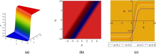
View original graphic|Download|PPT slide

Fig.1 (a), (b) stand for 3D, contour shapes for κ=0.25, α=λ=0.5, γ=0.8, ζ=μ=1, δ=-1, τ₁=0.2, y=0, in the range -10≤x,t≤10 while Fig 1(c) represents a class of 2D profiles with the different values of κ (green (κ=0.1), red (κ=0.2), pink (κ=0.3), blue (κ=0.4)) and t=2.

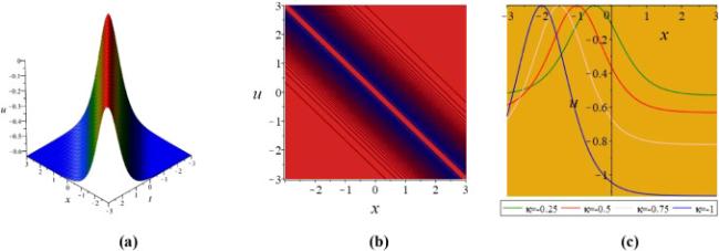
View original graphic|Download|PPT slide

Fig.2 (a), 2(b) stand for 3D, contour shapes for κ=-0.5, γ=τ₁=2, δ=-1, y=0, in the range -3≤x,t≤3 while Fig. 2(c) represents a class of 2D profiles with the different values of κ (green (κ=-0.25), red (κ=-0.5), pink (κ=-0.75), blue (κ=-1)) and t=1.

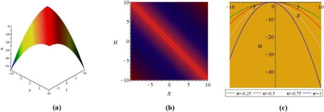
View original graphic|Download|PPT slide

Fig.3 (a), (b) within the interval -10≤x,t≤10 and the distinct values of κ (green (κ=-0.25), red (κ=-0.5), pink (κ=-0.75), blue (κ=-1)) and t=0.5 display diverse 2D profiles in Fig. 3(c).

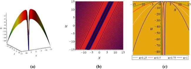
View original graphic|Download|PPT slide

Fig.4 (a), (b) stand for 3D, contour shapes for κ=0.25, γ=0.5, y=0, in the range -15≤x,t≤15 while Fig. 4(c) represents a class of 2D profiles with the different values of κ (green (κ=0.25), red (κ=0.5), pink (κ=0.75), blue (κ=1)) and t=1.

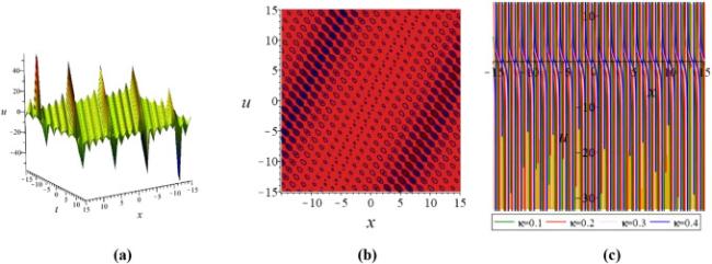
View original graphic|Download|PPT slide

Fig.5 (a), (b) stand for 3D, contour shapes for κ=0.25, α=0.5, λ=-1, γ=ζ=μ=1, y=0, in the range -15≤x,t≤15 while Fig. 5(c) represents a class of 2D profiles with the different values of κ (green (κ=0.1), red (κ=0.2), pink (κ=0.3), blue (κ=0.4)) and t=1.

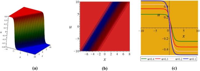
View original graphic|Download|PPT slide

Fig.6 (a), (b) within the interval -10≤x,t≤10 and the distinct values of κ (green (κ=0.4), red (κ=0.3), pink (κ=0.2), blue (κ=0.1)) and t=1 display diverse 2D profiles in Fig. 6(c).

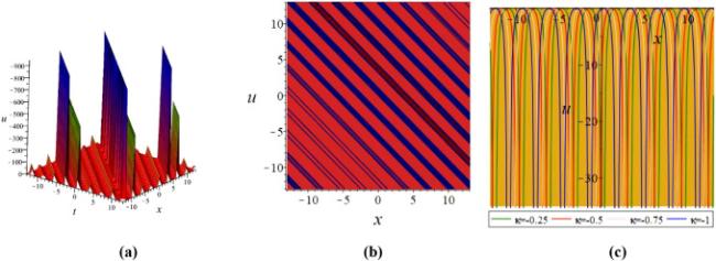
View original graphic|Download|PPT slide

Fig.7 (a), (b) stand for 3D, contour shapes for κ=-0.5, τ₀=1, τ₁=2, b=4, c=5, y=0, in the range -13≤x,t≤13 while Fig. 7(c) represents a class of 2D profiles with the different values of κ (green (κ=-0.25), red (κ=-0.5), pink (κ=-0.75), blue (κ=-1)) and t=1.

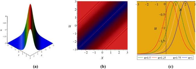
View original graphic|Download|PPT slide

Fig.8 (a), (b) stand for 3D, contour shapes for κ=0.5, b=4, c=3, y=0, in the range -3≤x,t≤3 while Fig. 8(c) represents a class of 2D profiles with the different values of κ (green (κ=0.5), red (κ=0.25), pink (κ=0.75), blue (κ=1)) and t=1.

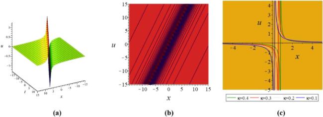
View original graphic|Download|PPT slide

Fig.9 (a), (b) within the interval -15≤x,t≤15 and the distinct values of κ (green (κ=0.4), red (κ=0.3), pink (κ=0.2), blue (κ=0.1)) and t=1 display diverse 2D profiles in Fig. 9(c).

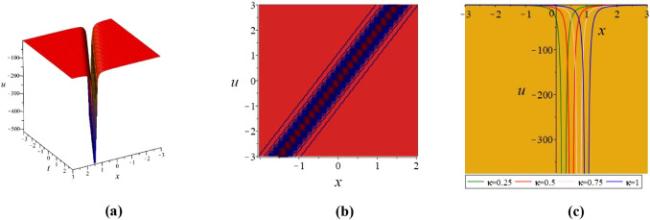
View original graphic|Download|PPT slide

Fig.10 (a), (b) stand for 3D, contour shapes for κ=0.25, y=0, in the range -3≤x,t≤3 while Fig. 10(c) represents a class of 2D profiles with the different values of κ (green (κ=0.25), red (κ=0.5), pink (κ=0.75), blue (κ=1)) and t=1.

5. Conclusions

In this study, the coupled nonlinear Maccari system has been studied and extracted analytic solutions of by means of two competent techniques namely improved tanh method and rational

(G^{'} / G)

-expansion scheme. Abundant closed-form soliton solutions are successfully generated in terms of rational, hyperbolic and trigonometric functions. The acquired solutions alongside particular values of involved free parameters are illustrated in 2D, 3D and contour traces to depict diverse soliton patterns. The soliton patterns are appeared as kink type, bell shape, periodic, compacton, cuspon, peakon, etc. Different wave propagations due to the change of wave velocity are brought out through various 2D outlines. The relative study of the obtained outcomes and the results available in the knowledge has made us to claim the novelty and diversity of the achieved solution in this work. The adopted tools have performed as concise, efficient and productive to make available a heap of exact solutions which might convey a significant contribution to depict the intrinsic behaviors of nonlinear natural phenomena. The future research relevant to this study considering the mentioned techniques and any nonlinear evolution equations is just waiting for a few moments.

Declaration of Competing Interest

The authors declare that they have no known competing financial interests or personal relationships that could have appeared to influence the work reported in this paper.

References

Publishing order | Descend order by publishing year | Descend order by cited within

[1]	A.M. Wazwaz. Partial Differential Equations: Method and Applications. Taylor and Francis ( 2002)

[2]	K.S. Miller, B. Ross. An Introduction to the Fractional Calculus and Fractional Differential Equations. Wiley, New York (1993)

[3]	A.A. Kilbas, H.M. Srivastava, J.J. Trujillo. Theory and Applications of Fractional Differential Equations. Elsevier, Amsterdam (2006)

[4]	M. Bilal, A.R. Seadawy, M. Younis, S.T.R. Rizvi, K. El-Rashidy, S.F. Mahmoud. Res. Phys., 23 ( 2021), Article 103959

[5]	A. Yokus, H.M. Baskonus, T.A. Sulaiman, H. Bulut. Numer. Method Partial Differ. Eq., 34 ( 2018), pp. 211-227 DOI: 10.1002/num.22192

[6]	M.T. Islam,M.A. Akter. J. Res. Eng. Appl. Sci., 6 (2021), pp. 11-18 DOI: 10.1117/12.2596325

[7]	H. Ahmad, A.R. Seadawy, T.A. Khan,P. Thounthong. J. Taibah Univ. Sci., 14 (2020), pp. 346-358 DOI: 10.1080/16583655.2020.1741943

[8]	Y. Hu, Y. Luo, Z. Lu. J. Comput. Appl. Math., 215 (2008), pp. 220-229

[9]	S. Kumar, A. Kumar, A.M. Wazwaz. Eur. Phys. J. Plus., 135 (2020), pp. 1-17

[10]	A. Akbulut, M. Kaplan, A. Bekir. Int. J. Nonlinear Sci. Numer. Simul., 17 ( 2016), pp. 413-420 DOI: 10.1515/ijnsns-2016-0023

[11]	H. Bulut, H.M. Baskonus, Y. Pandir. Abst. Appl. Anal. (2013), Article 6368022013

[12]	H.Y. Martinez, J.F.G. Aguilar, A. Atangana. Math. Model. Nat. Phenom., 13 (2018), p. 14

[13]	M.A. Akbar, N.H.M. Ali, M.T. Islam.AIMS Math., 4 (2019), pp. 397-411 DOI: 10.32520/stmsi.v8i3.521

[14]	W.X. Ma, J.H. Lee. Chaos Solitons Fractals, 42 (2009), pp. 1356-1363

[15]	A. Yokus, H. Durur, S. Duran. Opt. Quantum Electron., 53 (402) (2021), pp. 1-15

[16]	M.T. Islam, M.A. Akbar, A.K. Azad. J. Ocean. Eng. Sci., 3 (2018), pp. 76-81

[17]	S.T.R. Rizvi, A.R. Seadawy, M. Younis, S. Iqbal, S. Althobaiti, A.M. El-Shehawi. Res. Phys., 23 ( 2021), Article 103998

[18]	M.T. Islam, M.E. Islam, M.A. Akbar. Arab J. Basic Appl. Sci.,28 (2021), pp. 64-72 DOI: 10.1080/25765299.2021.1886678

[19]	M. Younis, N. Cheemaa, S.A. Mehmood, S.T.R. Rizvi, A. Bekir. Com. Med., 30 (2018), pp. 490-499

[20]	A. Bhalraj, A. Azmi, M.H. Mohd. Int. J. Math. Com. Sci., 16 (2021), pp. 949-961

[21]	A.A. Al-Shawba, K.A. Gepreel, F.A. Abdullah, A. Azmi. Res. Phys., 9 (2018), pp. 337-343

[22]	A. Ciancio, H.M. Baskonus, T.A. Sulaiman, H. Bulut. Indian J. Phys., 92 ( 2018), pp. 1281-1290 DOI: 10.1007/s12648-018-1204-6

[23]	M. Inc, A.I. Aliyu, A. Yusuf, D. Baleanu, E. Nuray. Mod. Phys. Lett. B, 32 (2018), Article 1850014

[24]	A. Neirameh. Alex. Eng. J., 55 (2016), pp. 2839-2847

[25]	H.M. Baskonus, T.A. Sulaiman, H. Bulut. Opt. (Stuttg), 131 (2017), pp. 1036-1043

[26]	H. Bulut, G. Yel, H.M. Baskonus. Adv. Math. Mod. Appl., 2 (2017), pp. 14-19

[27]	D. Rostamy, F. Zabihi. Nonlinear Studies, 19 (2012), pp. 229-239

[28]	J. Vahidi, S.M. Zekavatmand, H. Rezazadeh, M. Inc, M.A. Akinlar,Y. Chu. Res. Phys., 21 (2021), Article 103801

[29]	Y. Akbar, H. Afsar, S. Abbas, M.W. Javed,N. Ullah. Chaos Solitons Fractals, 150 (2021), Article 111114

[30]	A. Maccari. J. Math. Phys., 12 (1996), pp. 6207-6212

[31]	A. Jabbari, H. Kheiri, A. Bekir. Comput. Math. Appl., 62 (2011), pp. 2177-2186

[32]	M.M.A. Khater, A.R. Seadawy, D. Lu. J. King Saud Univ. Sci., 30 (2018), pp. 417-423

[33]	N. Cheemaa, S. Chen, A.R. Seadawy. Res. Phys., 17 ( 2020), Article 102987

[34]	L. Liu, B. Tian, Y.Q. Yuan, Y. Sun. Eur. Phys. J. Plus., 133 (2018), pp. 1-14

[35]	M.G. Hafez, B. Zheng, M.A. Akbar. Egypt. J. Basic Appl. Sci., 2 (2015), pp. 206-220 https://www.sciencedirect.com/science/article/pii/S2314808X15000214/pdfft?md5=e82da4c639b347a349811b4ebead87fd&pid=1-s2.0-S2314808X15000214-main.pdf DOI: 10.1016/j.ejbas.2015.04.002

[36]	M.M.A. Khater, M.S. Mohamed, R.A.M. Attia.Chaos Solitons Fractals, 144 (2021), Article 110676

[37]	Y. Chu, M.M.A. Khater, Y.S. Hamed. AIP Adv., 11 (2021), Article 015223

[38]	M.M.A. Khater, A.E. Ahmed, M.A. El-Shorbagy.Results Phys., 22 (2021), Article 103890

[39]	M.M.A. Khater, A.E. Ahmed, S.H. Alfalqi, J.F. Alzaidi, S. Elbendary, A.M. Alabdali.Results Phys., 25 (2021), Article 104322

[40]	M.M.A. Khater, A.A. Mousa, M.A. El-Shorbagy, R.A.M. Attia.Results Phys., 22 (2021), Article 103954

[41]	M.M.A. Khater, K.S. Nisar, M.S. Mohamed. Math. Met. Appl. Sci., 44 (6) (2021), pp. 4598-4606 DOI: 10.1002/mma.7052

[42]	M.M.A. Khater, B. Ghanbari. Eur. Phys. J. Plus, 136 (447) (2021), pp. 1-28 DOI: 10. 3138/diaspora.21.1.2020-06-15

[43]	M.M.A. Khater, T.A. Nofal, H.A. Zinadah, M.S.M. Lotayife, D. Lu. Alex. Eng. J., 60 (2021), pp. 1797-1806

[44]	M.M.A. Khater, M.S. Mohamed, S.K. Elagan. Results Phys., 23 (2021), Article 104003

[45]	M.M.A. Khater, S. Anwar, K.U. Tariq, M.S. Mohamed. AIP Adv., 11 (2021), Article 025130

[46]	M.M.A. Khater, A. Bekir, D. Lu, R.A.M. Attia. Math. Met. Appl. Sci., 44 (3) (2021), pp. 2682-2691 DOI: 10.1002/mma.6951

[47]	M.M.A. Khater, A.A. Mousa, M.A. El-Shorbagy, R.A.M. Attia. Eur. Phys. J. Plus., 136 (604) ( 2021), pp. 1-11 DOI: 10. 3138/diaspora.21.1.2020-06-15

[48]	M.M.A. Khater, S.K. Elagan, A.A. Mousa, M.A. El-Shorbagy, S.H. Alfalqi, J.F. Alzaidi,D. Lu. Results Phys., 25 (2021), Article 104133

[49]	R.A.M. Attia, M.M.A. Khater, A.E. Ahmed, M.A. El-Shorbagy. AIP Adv., 11 (2021), Article 055105

[50]	M.M.A. Khater. Mod. Phys. Lett. B, 35 (22) ( 2021), Article 2150372 DOI: 10.1142/s0217984921503723

[51]	M.M.A. Khater, A.E. Ahmed, S.H. Alfalqi, J.F. Alzaidi. Phys. Scr., 96 (7) (2021), Article 075207

[52]	M.M.A. Khater, D. Lu. Mod. Phys. Lett. B, 35 (19) ( 2021), Article 2150324 DOI: 10.1142/s0217984921503243

[53]	M.M.A. Khater, A.E. Ahmed.AIMS Math., 6 (6) (2021), pp. 5896-5908 DOI: 10.3934/math.2021349

[54]	M.M.A. Khater, L. Akinyemi, S.K. Elagan, M.A. El-Shorbagy, S.H. Alfalqi, J.F. Alzaidi, N.A. Alshehri.Symmetry (Basel), 13 (2021), p. 963 DOI: 10.3390/sym13060963

[55]	C. Yue, D. Lu, M.M.A. Khater. Fluids, 6 (7) ( 2021), p. 235 DOI: 10.3390/fluids6070235

[56]	W. Li, L. Akinyemi, D. Lu, M.M.A. Khater.Symmetry (Basel), 13 (2021), p. 1085 DOI: 10.3390/sym13061085

[57]	M.M.A. Khater, A.M. Alabdali. Mathematics, 9 ( 2021), p. 1440 DOI: 10.3390/math9121440

[58]	P. Veeresha, D.G. Prakasha, N. Magesh, A.J. Christopher, D.U. Sarwe. J. Ocean Eng. Sci., 6 (3) (2021), pp. 265-275

[59]	R.M. El-Shiekh, M. Gaballah. J. Ocean Eng. Sci., 5 (2) (2020), pp. 180-185

[60]	A. Vithya, M.S.M. Rajan. J. Ocean Eng. Sci., 5 (3) (2020), pp. 205-213

[61]	M.M. Miah, A.R. Seadawy, H.M.S. Ali, M.A. Ali. J. Ocean Eng. Sci., 5 (3) (2020), pp. 269-278

[62]	R.M. El-Shiekh, M. Gaballah. J. Ocean Eng. Sci., 5 (2) (2020), pp. 180-185

[63]	M.P. Haghighi, J. Manafian. J. Ocean Eng. Sci., 5 (3) (2020), pp. 197-204

[64]	M.A. Shallal, K.K. Ali, K.R. Raslan, H. Rezazadeh, A. Bekir. J. Ocean Eng. Sci., 5 (3) (2020), pp. 223-229

[65]	M.T. Islam, M.A. Akter. Partial Differ. Eq. Appl. Math., 3 ( 2021), Article 100031

[66]	M.T. Islam, M.A. Akbar, M.A.K. Azad. Nonlinear Stud., 6 (2015), pp. 1-11

Options

Abstract

Outlines

模态框（Modal）标题

Abstract

Cite this article

1. Introduction

2. Explanation of the methods

2.1. The improved tanh method

2.2. The rational (G′/G) -expansion method

3. Formulation of solutions

3.1. The improved tanh method

3.2. The rational (G′/G) -expansion method

4. Results discussion and graphical representations

Fig.1 (a), (b) stand for 3D, contour shapes for κ=0.25, α=λ=0.5, γ=0.8, ζ=μ=1, δ=-1, τ1=0.2, y=0, in the range -10≤x,t≤10 while Fig 1(c) represents a class of 2D profiles with the different values of κ (green (κ=0.1), red (κ=0.2), pink (κ=0.3), blue (κ=0.4)) and t=2.

Fig.2 (a), 2(b) stand for 3D, contour shapes for κ=-0.5, γ=τ1=2, δ=-1, y=0, in the range -3≤x,t≤3 while Fig. 2(c) represents a class of 2D profiles with the different values of κ (green (κ=-0.25), red (κ=-0.5), pink (κ=-0.75), blue (κ=-1)) and t=1.

Fig.3 (a), (b) within the interval -10≤x,t≤10 and the distinct values of κ (green (κ=-0.25), red (κ=-0.5), pink (κ=-0.75), blue (κ=-1)) and t=0.5 display diverse 2D profiles in Fig. 3(c).

Fig.4 (a), (b) stand for 3D, contour shapes for κ=0.25, γ=0.5, y=0, in the range -15≤x,t≤15 while Fig. 4(c) represents a class of 2D profiles with the different values of κ (green (κ=0.25), red (κ=0.5), pink (κ=0.75), blue (κ=1)) and t=1.

Fig.5 (a), (b) stand for 3D, contour shapes for κ=0.25, α=0.5, λ=-1, γ=ζ=μ=1, y=0, in the range -15≤x,t≤15 while Fig. 5(c) represents a class of 2D profiles with the different values of κ (green (κ=0.1), red (κ=0.2), pink (κ=0.3), blue (κ=0.4)) and t=1.

Fig.6 (a), (b) within the interval -10≤x,t≤10 and the distinct values of κ (green (κ=0.4), red (κ=0.3), pink (κ=0.2), blue (κ=0.1)) and t=1 display diverse 2D profiles in Fig. 6(c).

Fig.7 (a), (b) stand for 3D, contour shapes for κ=-0.5, τ0=1, τ1=2, b=4, c=5, y=0, in the range -13≤x,t≤13 while Fig. 7(c) represents a class of 2D profiles with the different values of κ (green (κ=-0.25), red (κ=-0.5), pink (κ=-0.75), blue (κ=-1)) and t=1.

Fig.8 (a), (b) stand for 3D, contour shapes for κ=0.5, b=4, c=3, y=0, in the range -3≤x,t≤3 while Fig. 8(c) represents a class of 2D profiles with the different values of κ (green (κ=0.5), red (κ=0.25), pink (κ=0.75), blue (κ=1)) and t=1.

Fig.9 (a), (b) within the interval -15≤x,t≤15 and the distinct values of κ (green (κ=0.4), red (κ=0.3), pink (κ=0.2), blue (κ=0.1)) and t=1 display diverse 2D profiles in Fig. 9(c).

Fig.10 (a), (b) stand for 3D, contour shapes for κ=0.25, y=0, in the range -3≤x,t≤3 while Fig. 10(c) represents a class of 2D profiles with the different values of κ (green (κ=0.25), red (κ=0.5), pink (κ=0.75), blue (κ=1)) and t=1.

5. Conclusions

References

Links

2.2. The rational $(G^{'} / G)$ -expansion method

3.2. The rational $(G^{'} / G)$ -expansion method

Fig.1 (a), (b) stand for 3D, contour shapes for κ=0.25, α=λ=0.5, γ=0.8, ζ=μ=1, δ=-1, τ₁=0.2, y=0, in the range -10≤x,t≤10 while Fig 1(c) represents a class of 2D profiles with the different values of κ (green (κ=0.1), red (κ=0.2), pink (κ=0.3), blue (κ=0.4)) and t=2.

Fig.2 (a), 2(b) stand for 3D, contour shapes for κ=-0.5, γ=τ₁=2, δ=-1, y=0, in the range -3≤x,t≤3 while Fig. 2(c) represents a class of 2D profiles with the different values of κ (green (κ=-0.25), red (κ=-0.5), pink (κ=-0.75), blue (κ=-1)) and t=1.

Fig.7 (a), (b) stand for 3D, contour shapes for κ=-0.5, τ₀=1, τ₁=2, b=4, c=5, y=0, in the range -13≤x,t≤13 while Fig. 7(c) represents a class of 2D profiles with the different values of κ (green (κ=-0.25), red (κ=-0.5), pink (κ=-0.75), blue (κ=-1)) and t=1.