
1. Introduction
Nonlinear evolution equation is a research hotspot in different fields of science and engineering especially in energy and material science topics [1], [2], [3], [4], [5], [6], [7], [8], [9], [10], [11], [12], [13], [14]. No doubt experts have made remarkable achievements in these fields. So far, a variety of analytical and numerical schemes have been introduced to analyze and solve nonlinear evolution equations (NLEEs), the most typical of which include the unified method and its generalized form [15], [16], the tanh-coth-expansion and sine-cosine-function methods [17], [18], the -expansion method [19], [20], [21], sine-Gordon expansion method [22], [23], the modified Kudryashov method [24], [25], [26], the Hirota bilinear method [27], [28], [29], [30], [31], the finite difference method [32], the Riccati equation technique [33], the modified reproducing kernel discretization technique [34], the long wave limit method [35], the cubic B-spline scheme [36], the q-homotopy analysis [37] and the bilinear neural network method [38], [39], [40], [41]. In this research, we examine the dynamical behavior of a minor element achieved through the phase decomposition of the main element in a binary alloy which is completely described by the Cahn-Hilliard (CH) system [42], [43] via the unified method [44], [45], [46]. To this end, many exact solutions are created for this model and the physical meanings for the obtained solutions are illustrated by two- and three-dimensional figures and their contour plots.
where , , represents uphill diffusion, and is the total free energy. Further, the CH equations can be written as
where represents the homogeneous free energy and is a constant. The system (2) admits the convective-diffusive CH equation [48]
where and represent the concentration and the mobility, respectively. Consequently, Eq. (3) can be written in the next formula [47]
where is a substantial chemical potential that has a common illustration as and denotes the concentration of one of two phases in a phase transitioning system. , on the other hand, describes the phase shift caused by the fluid flow in a steady state. Eq. (4) covers the phase transition in binary systems such as glass and polymer mixtures as well as the kinetics of phase separation in iron-based ternary alloys.
Herein, The study of Eq. (4) is investigated when its coefficients are functions of the time. This discussion has attracted much attention rather than the constant case, since the majority of nonlinear physical equations in practice have variable coefficients. To this end we assume Eq. (4) with variable coefficients in the form:
where , and are real arbitrary functions.
The reminder of the article has been organized by the following next three Sections: Section 2 is dedicated to the unified method construction. The utilizing of the aforemention method on our problem and the analysis of the dynamical properties for the obtained solutions through some figures are investigated in Section 3, while Section 4 will contain the conclusion and results.
2. A short note on the unified method
In this part, we illustrate the algorithm of the unified method by introducing the following nonlinear differential equation with variable coefficients:
Applying the wave transformation into (6). Thus, Eq. (6) becomes an ordinary differential equation with the form:
where is a real constant, is an arbitrary function, and .
2.1. The polynomial type of wave solutions
This kind of solutions takes the following form
where are arbitrary functions in and the auxiliary function satisfies the following auxiliary equation
where are arbitrary functions in and gives elementary or implicit solutions for Eq. (9), while gives periodic or elliptic solutions. The homogeneous balancing requirement between the highest order derivative and highest nonlinear terms of Eq. (7) specifies the values of and when . We mention that the value of depends basically on the parameters , and the highest derivative, say , of Eq. (7). The parameter is the total number of algebraic equations resulting from inserting Eqs. (8) and (9) into Eq. (7) and equating the coefficients of with different powers identical zero. While, the parameters represents the number of free parameters in Eqs. (8) and (9). Thus the condition for finding is given by when Eq. (7) is integrable.
2.2. The rational type of wave solutions
The unified method suggests the rational type of wave solutions as follow:
where and are arbitrary functions in and the auxiliary function satisfies the same auxiliary Eq. (9). The same technique in the previous case can be followed to obtain this type of solutions for Eq. (7).
In this work, we confine ourselves to discuss the solutions of Eq. (5) in the polynomial type. While the rational type solutions for this equation will investigate in a future work under the affect of the conformable derivative.
3. Solutions of Eq. (5) via the unified method
In the current part, we construct a variety of closed-form solutions with different structures for suggested Eq. (5).
To solve the model we have described, we apply the following wave transformation . Substituting this transformation into Eq. (5) gives the new nonlinear ODE:
wherein prime indicates differentiation with respect to the new parameter . On the other hand, if Eq. (11) is integrated and the integral constant is ignored, the following equation is easily obtained
3.1. Implementation of the polynomial solutions
Consider Eq. (8) as a solution of Eq. (12). After balancing the highest order derivative term with the highest nonlinear term in (12), we get and the consistency condition states that .
Type I When and or
Case 1. Solitary wave solution (when )
In this case, according to the relation , and the general solution of Eq. (12) takes the form
where satisfies the auxiliary equation
Plugging Eqs. (13) and (14) into Eq. (12) and equating all coefficients of , we get a system of algebraic equations that can be solved as follow:
where and . Thus, the solution of Eq. (5) takes the form:
Fig. 1 depicts a special symmetric solitary wave with unique maximum value, which is symmetric about the origin. Further, this solutions approaches zero when . The geometrical structure of this solution represents a bright-dark wave solution.
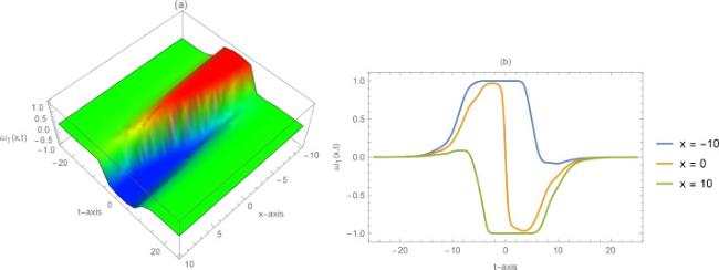
Fig.1 The solitary wave solution given by (16) in 3D and 2D plots for , . |
Case 2. M-type wave solution (when )
In this case, according to the relation , and the general solution of Eq. (12) takes the form
where satisfies the auxiliary equation
Plugging Eqs. (17) and (18) into Eq. (12)and equating all coefficients of , we get a system of algebraic equations that can be solved as follow:
where . Thus, the solution of Eq. (5)takes the form:
Fig. 2 shows a periodic M-shaped wave solution which is created due to changing the sign of the coefficient related to the weak dispersion. The peak value at the upper side is smaller than the absolute value of the peak value at the lower side.
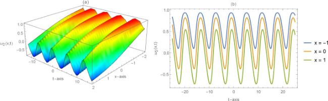
Fig.2 The M-type wave solution given by (20) in 3D and 2D plots for , . |
Type II When and
Case 1. Elliptic wave solution
In this case, according to the relation , and the general solution of Eq. (12) takes the form
where satisfies the auxiliary equation
Without losing the generality, we take in Eq. (22).
Plugging Eqs. (21) and (22) into Eq. (12) and equating all coefficients of and , we get a system of algebraic equations that can be solved as follow:
where . Thus, the solution of Eq. (5) takes the form:
where satisfies Eq. (22).
We mention that Eq. (22) has a variety of possible solutions in Jacobi elliptic functions type according to the choices of the arbitrary functions . So, we take . From the classification existed in Zhang [49], we take
where is the modulus of the Jacobi elliptic function. When or , the Jacobi elliptic function degenerates into or , respectively.
Substituting Eq. (25) into Eq. (24), we get the final solution shape of Eq. (5) as follows
Figs. 3 and 4 depict special kinds of elliptic waves namely conoidal and chirped wave solutions when the modulus of the Jacobi elliptic function and , respectively.
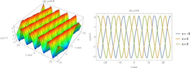
Fig.3 The Elliptic wave solution given by (26) in 3D and 2D plots for . |
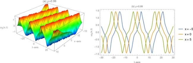
Fig.4 The Elliptic wave solution given by (26) in 3D and 2D plots for . |
Case 2. Periodic wave solution
Here, the solution has the same structure in Eq. (21) but with different auxiliary equation given by
Plugging Eqs. (21) and (27) into Eq. (12) and equating all coefficients of and , we get a system of algebraic equations that can be solved as follow:
where . Consequently, the solution of Eq. (5) takes the form:
Fig. 5 shows a mixed breather-lump periodic wave solution with stable amplitude. This wave is symmetric about the origin and propagates parallel to the -axis.
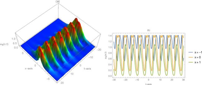
Fig.5 The Periodic wave solution given by (29) in 3D and 2D plots for , . |
4. Conclusion
Herein, the main goal of this work is to exploit the unified method to attain new nonautonomous explicit and implicit wave solutions of the Cahn-Hilliard system when its coefficients varying with time in the area of mathematical physics, especially the field of energy and materials sciences. The obtained solutions are obtained in the polynomial type with different geometrical structures namely: bright-dark, M-type, conoidal soliton, chirped, and mixed breather-lump periodic wave solutions. The dynamical behaviors for these solutions in self-phase modulation medium are analyzed graphically through two-dimensional and three-dimensional graphics for different choices of the free parameters and arbitrary functions existed in the solutions. Our preferred method is capable of reducing the size of computational estimates and can be easily applied to a variety of physical challenges in the fields of theoretical physics and engineering. The data obtained demonstrate the effectiveness, simplicity and efficiency of the unified method.
Declaration of Competing Interest
Authors declare that they have no conflict of interest.
