
1. Introduction
As the exploration of the marine environment gains increasing importance, marine crafts have received considerable attention for their versatility in supporting various marine missions [1]. Consequently, these marine crafts, with their diverse capabilities, have become essential in facilitating a wide range of marine activities and objectives [2]. Central to their operation is the motion model, a crucial element necessary for designing accurate and reliable control systems.
Given its importance, an accurate motion model is vital as it significantly influences the effectiveness of the crafts' performance. Moreover, deviations from the true motion model could potentially degrade control performance or, in the worst case, lead to critical safety issues [3]. Currently, motion modeling of marine crafts has become a vital point, emerging as a prominent area of research in marine technology [4].
Creating motion models for marine crafts is complex, impacted by factors such as the unpredictability of the ocean and water viscosity. Specifically, predicting the effects of ocean waves, currents, and water viscosity on the craft is challenging. Waves, being constantly changing, make accurate modeling difficult [5]. Additionally, currents further complicate the modeling process by affecting the craft's trajectory and stability. Khater emphasizes the challenges in modeling water movements in varying channels and underscores the need for sophisticated calculations [6]. Similarly, water viscosity significantly impacts marine craft motion modeling, influencing drag forces and thus affecting speed and maneuverability.
These environmental conditions add complexity and variability to the crafts' motion, posing challenges to the modeling process [7]. Nowadays, motion modeling can be classified into three categories, namely mechanism modeling, identification modeling, and mechanism-identification hybrid modeling. Among these, mechanism modeling, which uses motion laws to explain physical processes, effectively describes specific motion mechanisms [8]. Besides, the empirical formula method (EFM) plays a crucial role in mechanism modeling. It relies on historical data and empirical formulas derived from prior experiments and operational experiences, which allows EFM to estimate various motion parameters of marine crafts, especially when utilizing existing shape databases. However, it's important to note that the accuracy of EFM depends on the completeness and relevance of these databases. When applied to less-represented marine craft shapes, its prediction accuracy can significantly decrease to about 75% [9]. This indicates a level of uncertainty in the model predictions for unconventional or new marine craft designs, making it essential to continually update and expand the shape databases to improve the method's applicability and accuracy in motion modeling of diverse marine crafts.
Compared with mechanism modeling, which typically relies on established physical principles, identification modeling directly uses motion data [9]. Among identification modeling methods, the constrained model testing method (CMT) has gained popularity [10]. In CMT, physical models of marine crafts are tested under controlled conditions to simulate real-world behavior and motion characteristics. The models are subjected to constraints, enabling the collection of data that accurately reflects marine craft performance. Methods like CMT can provide valuable insights into marine craft behaviors under specific conditions, but they often require extensive testing to generate comprehensive datasets for improved model accuracy and reliability.
Additionally, black-box modeling based on system identification is widely used. For instance, Zhang et al. [11] employed multi-output support vector regression for black-box modeling, incorporating three levels of white noise into raw simulation data for training. Similarly, Jiang et al. [12] constructed a neural network-based black-box model for ship maneuvering using experimental data. However, the accuracy of identification modeling is heavily reliant on large sample data sets.
Consequently, the mechanism-identification hybrid modeling strategy has become increasingly popular in marine craft motion modeling [13], [14], [15]. This approach leverages the mechanism to establish equations of motion, and identification algorithms are utilized to obtain model parameters. Therefore, the mechanism-identification hybrid modeling achieves higher accuracy than mechanism modeling and requires fewer sample data than identification modeling.
Developing a mechanism-identification hybrid model that combines mechanism and identification approaches requires careful planning and execution. Researchers must select and design three key elements: the mathematical model, the input and output data, and the identification algorithm [13]. Adding to this, the computational fluid dynamics method (CFD) enriches the hybrid modeling strategy by bringing in a more sophisticated simulation of fluid-structure interactions [16]. The CFD allows for a detailed examination of the marine craft's behavior within its operational fluid environment, enabling a more precise representation of real-world conditions. Unlike traditional mathematical models, CFD captures complex nonlinear dynamics by solving Navier-Stokes equations and considering turbulence models for flow analysis around the hull [17]. Although CFD brings advanced simulation capabilities and detailed insights into fluid-structure interactions, there are significant limitations associated with CFD. One of the main limitations is the high computational cost [18]. CFD simulations require substantial computational resources and time, making them less efficient, especially when dealing with real-time applications or when multiple iterations are needed. Additionally, CFD models are complex and require a high level of expertise to handle and interpret the results correctly. Moreover, the detailed setup of CFD simulations, including mesh generation and turbulence modeling, requires extensive resources and expertise, potentially limiting its utility in certain scenarios.
In the field of mathematical models, both linear and nonlinear models have been explored and proposed by scholars. In particular, linear models, such as the well-known Nomoto rudder-yaw model, have proven effective in capturing the dynamics of marine crafts under standardized conditions, such as fixed maneuvers and constant cruising speeds [19]. A variety of methods have also been introduced for parameter identification within these linear frameworks, such as the least squares method [20] and the Kalman filter algorithm [21], [22]. A noteworthy application of the latter was presented by Zare et al. who used the Kalman filter algorithm to identify specific parameters of an autonomous underwater vehicle using the autoregressive moving average model [23]. The results had a commendable level of accuracy within the simulated environment. However, despite their usefulness, linear models have certain limitations, particularly in their predictive capabilities. Their architectural design restricts them from accurately capturing the more complex and nonlinear dynamics inherent in marine craft's motion. This limitation presents challenges in the pursuit of a more accurate motion modeling approach.
Nonlinear models are proved to be superior when dealing with non-linear problems, displaying remarkable adaptability and precision [24]. They have a heightened ability to grasp the complexities and variations encountered during navigation, adjusting to changes in cruising speeds and rudder angles effectively [25], [26]. This flexibility allows for a more realistic representation of dynamic behaviors experienced in marine environments. Recently, several parameter identification algorithms have been proposed and tested based on the nonlinear model. For instance, in [27], the Abkowitz model was chosen to highlight hydrodynamic characteristics, and a support vector machine algorithm was employed for parameter identification. Compared to the traditional support vector machine algorithm, the least squares support vector machine (LS-SVM) algorithm has simpler and fewer constraints [28]. Building on the LS-SVM algorithm, Hu et al. [29] accomplished parameter identification using the Abkowitz model. Numerical simulations demonstrated that the LS-SVM algorithm effectively obtained hydrodynamic coefficients. However, the nonlinear model encompasses a richer set of hydrodynamic and coupling states than the linear model [30], which may lead to issues such as parameter drift and cancellation. Consequently, a balance between model complexity and parameter identification accuracy is required.
Specifically, the least squares (LS) method is one of the most widely used identification algorithms in science and engineering, available for both linear and nonlinear models. Intuitively, the LS algorithm aims to find a vector that minimizes the Euclidean norm , where is the regressor matrix and is the output vector. However, when is contaminated with noise, the results obtained by the LS algorithm may deviate significantly from the true value [31]. Since noise cannot be avoided in experiments, measurement noise should be taken into account.
Enhancing the accuracy of parameter identification with measurement noise is imperative, necessitating innovative approaches and algorithms. A multi-sensor least-squares parameter identification algorithm has been proposed previously [32], which considers uncorrelated white noise. To further mitigate noise effects, the variance of Gaussian white noise was estimated in [33]. The performance of the LS-based parameter identification algorithm was verified based on data from water tank tests. Although it is generally assumed that there is only white noise in the system, many real measurement scenarios involve colored noise [34], [35]. Ding et al. [36] treated the noise as colored measurement noise and processed it using a moving average model. Madapusi et al. [37] proposed a quadratic constrained least squares estimator with a semidefinite constraint matrix for parameter identification under colored noise. However, this algorithm assumes prior knowledge of the noise covariance matrix, which is often impractical. Consequently, parameter identification of marine crafts without prior noise information remains an area deserving further research.
Motion prediction of marine crafts is highly valued for evaluating model accuracy and improving motion safety. However, predicting these motions is challenging due to changes in speed and external disturbances. Recently, many motion prediction strategies have been proposed, which can be roughly divided into data-driven and model-based algorithms [38]. Neri [39] proposed a time-domain simulator for short-term ship motion prediction based on data from the voyage data recorder, where a reliable linear regression scheme was implemented. However, the ship position prediction was limited to only 40 s. In [40], a methodology was developed for relatively long-term motion prediction based on a short-term memory neural network, but large amounts of motion data are required for accurate prediction. In contrast, model-based algorithms require limited motion data and can achieve long prediction times. Liu et al. [41] proposed an online LS-SVM algorithm for ship deck motion prediction, which achieved promising prediction performance with limited sea trial data and a deck-motion model. Nevertheless, few studies have focused on predicting the diving motion of marine crafts.
Building upon the considerations mentioned above, this paper strategically embraces the concept of system identification technique based on mechanism-identification hybrid modeling, aiming to innovatively bridge the current research gaps in diving motion predictions of marine crafts. Essential to the motion prediction framework is the integration of an anti-noise least squares algorithm that effectively reduces noise, thereby enhancing the robustness of our system against noise contamination,which has traditionally undermined the credibility and accuracy of identification. Specifically, this paper covers the following three aspects in-depth:
● A system identification technique based on a mechanism-identification hybrid model is applied for the diving motion prediction of marine crafts. Compared to data-driven algorithms, such as those in [42], this technique has lower requirements for data quality and length. Furthermore, unlike the methods detailed in [4], [43], it approximates actuator-related characteristics using a nonlinear equation, which further improves the modeling accuracy of diving dynamics.
● Building upon the recursive weighted least squares (RWLS) algorithm, an instrumental variable-based least squares (IVLS) algorithm is proposed for system identification. This algorithm significantly enhances the independence between noise and sample data, thereby improving its resistance to measurement noise. Its effectiveness is further demonstrated through the preliminary probabilistic proof of parameter convergence, even in models that include noise. This marks a notable advancement over methodologies such as those described in [37], as the IVLS algorithm operates efficiently without necessitating prior knowledge about the noise, broadening its real-world applications.
● The IVLS algorithm is innovatively applied for accurate parameter identification and motion prediction in marine crafts using field data, extending the work of [44]. It is evaluated using four depth control datasets from Qiandao Lake. Comparative results show that the proposed IVLS algorithm outperforms the RWLS and LS-SVM algorithms in multi-depth motion prediction, as demonstrated by lower average absolute error (AVGAE), root mean square error (RMSE), and maximum absolute error values and higher determination coefficient ( ).
The paper is organized as follows: Section 2 outlines the diving model of marine crafts and the corresponding parameter identification matrix. Section 3 describes the derivation of the IVLS algorithm and its stability analysis. Section 4 verifies the outperformance of the proposed IVLS algorithm over the RWLS and LS-SVM algorithms using field data. The final section gives conclusions and future work.
2. Model description
Marine crafts typically have highly nonlinear and coupled dynamics with six degrees of freedom. Traditionally, their dynamics model can be expressed as [45]:
where is the mass matrix; and represent the velocity and acceleration vectors respectively, encompassing linear and angular components; signifies the Coriolis and centripetal matrix; is the damping matrix, capturing resistance such as hydrodynamic drag; represents gravitational and buoyancy forces; symbolizes the vector of external forces and moments acting on the body, such as actuators, wind, and wave forces. represents the generalized velocity vector. It consists of both translational and rotational velocities. In detail, are the linear velocities in the body' local coordinate frame along the x, y, and z axes, and are the angular velocities about the same axes, depicting the body's rotational motion. Moreover, is the position and orientation vector. represent the position in the global frame, and indicate the body's orientation.
Focusing on the diving motion, the third row from the overall six-degree-of-freedom equations is selected, resulting in:
where represents the first derivative of velocity in the direction and denotes the body mass. The variables and denote the first derivatives of the angular velocities. The terms and define the positions of the center of gravity relative to the body coordinate system's origin. Damping coefficients in the direction are represented by (linear) and (quadratic), denotes the net buoyancy, signifies the external force, and is the actuator force acting in the direction.
However, managing and analyzing these dynamics can be technically challenging and computationally demanding. In this case, a simplified approach is feasible for diving motions, paving the way for a more efficient operational framework. This simplification depends on certain key configurations and assumptions:
● Metacentric height: The craft should have a significant metacentric height, implying a notable vertical distance between its center of gravity and buoyancy, thus enhancing attitude stability during navigation.
● Geometrical structure: The craft designed with a vertically elongated body, resembling a cylinder or an elliptical cylinder, facilitates better vertical stability due to a minimized horizontal flow resistance, making it easier to maintain an upright position.
● Internal mass distribution: An even distribution of mass within the craft is essential to avoid significant lateral mass imbalances that could compromise stability.
● Actuation considerations: The power system should primarily control the up and down motion of the craft, without significantly affecting other directions or rotations. This configuration makes the model simpler and more specialized for vertical motion.
● Motion speed: The motion should be characterized by a slower speed. This consideration allows simplification of the model dynamics while maintaining accuracy and reliability.
where is the body mass, is the additional mass, is the hydrodynamic damping coefficient, is the net buoyancy, is the external disturbance and unmodeled dynamics, and is the force generated by an on-board actuator. In this work, the actuator dynamic is approximated by
where and are three actuator-related coefficients and is the corresponding control signal. For a piston-driven buoyancy system equiped on the profiling float, is the piston position [44].
Then, Eq. (3) can be rewritten as
where and .
To establish a mechanism model for parameter identification of the piston-driven profiling float, Eq. (5) is discretized using the backward Euler method:
Here, is the sampling period between two sample points and is the time stamp.
Substituting Eq. (6) into Eq. (5) yields
with
Herein, is the output, is the input matrix and is the parameter matrix to be identified.
Remark 1: The fraction-based design of Eq. (8) can minimize the correlation between each input term in order to suppress the effect of parameter drift. On the other hand, the acquisition of accurate can be avoided and only five parameters need to be identified for diving dynamics with six coefficients.
3. Algorithm derivation and stability analysis
3.1. Derivation of the RWLS algorithm
In this subsection, the derivation of the above mentioned RWLS algorithm is carried out.
Firstly, criterion function of the RWLS algorithm is described by
where , and are given by
and is the weighting factor with being the number of sampling points.
Secondly, assuming , can be calculated
Thirdly, is defined as
Substituting Eq. (12) into Eq. (11) yields
To obtain the recursive form of , Eq. (13) is rewritten using
Fourthly, for fear of the inversion of in Eq. (14), is defined by
which can be further rewritten as
Moreover, to simplify Eq. (14), the identification gain is defined by
which can be transformed into
Accordingly, substituting Eq. (18) into Eq. (16), it obtains that
Finally, resorting to Eqs. (14), (18) and (19), the RWLS algorithm is summarized by
3.2. Stability analysis of the RWLS algorithm
Lemma 1: For the model , the RWLS-based identification result can consistently converge to the true value , i.e.
Proof:
The parameter identification error is defined by
Substituting in Eqs. (20) to (21) yields
and then using Eqs. (15) and (17), it has
Considering , Eq. (23) can be rewritten as
Letting
and being the eigenvalue of , it has
where is the non-zero eigenvector of .
Therefore, combining Eqs. (25) with (26) gives
Since and are semi-positive matrixes, and are of the same sign for all non-zero vector . Accordingly, the following equation holds
On the basis of Eq. (28), the system is stable, i.e.
Therefore, the proof is complete.
3.3. Derivation of the IVLS algorithm
However, the sample data will be contaminated with noise in practice. For this reason, the identification model in the presence of noise can be updated by
where is the measurement noise. In this case, Eq. (22) should be updated by
It's obvious that there is a high correlation exists between and , primarily because is dependent on and is influenced by the noise term . Consequently, the last term in Eq. (30) is non-zero from a probabilistic perspective, and thus the convergence of identification results for Eq. (30) cannot be guaranteed. Given this, the IVLS algorithm is further developed to enhance the independence between and .
Initially, the instrumental vector is constructed based on Eq. (8) as:
In the above equation, in Eq. (8) is replaced by the instrumental variable . This substitution improves the independence of and . Besides, is expressed by
Here, represents the smoothing factor, the time-lag coefficient, and is determined from Eq. (20).
Employing Eq. (32), in Eq. (18) is revised as:
Thus, part of is replaced by the instrumental vector by the instrumental variable . This rationale is the basis for labeling the algorithm as an instrumental variable-based least squares algorithm.
Remark 2: In Eq. (32), is estimated using the instrumental variable , and the time-lag coefficient is introduced to further mitigate the correlation between in Eq. (33) and in Eq. (29), thereby stabilizing the system characterized by Eq. (30). Finally, synthesizing Eqs. (20), (32), and (33), the IVLS algorithm is summarized as
Remark 3: The stability analysis of identification algorithms, such as those based on neural networks and support vector machine algorithms, has rarely been studied. In contrast, this paper preliminarily demonstrates the anti-noise stability of the IVLS algorithm from a probabilistic point of view.
Fig. 1 illustrates the procedure for IVLS-based parameter identification. The light orange box represents the diving model of the marine craft, the light green box denotes the discrete parameter identification matrix, the yellow box represents the IVLS algorithm, and the light blue box reflects the motion inversion using field data.
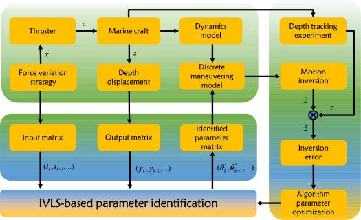
Fig.1 Block diagram of the parameter identification. |
4. Field data-based performance validation
where is the weighting vector in the high dimensional space and denotes the bias. Subsequently, the LS-SVM objective function is then defined as
where is the penalty factor and indicates the regression error.
Using the Karush-Kuhn-Tucker condition [29] and the linear kernel function , the regression model is obtained. Additionally, the parameter identification results are obtained using the input and output matrix given in Eq. (8).
Due to the unknown actual parameters of the motion mechanism model, it is difficult to accurately evaluate the accuracy of the identified parameters. Therefore, motion inversion and prediction are performed to evaluate the accuracy of the parameters identified by the IVLS algorithm. A small error in motion inversion and prediction indicates excellent accuracy in parameter identification. To illustrate these procedures visually, a diagram is shown in Fig. 2. First, the identified parameters are inputted into Eq. (5) to generate the identified diving model. Then, the identified model is fed with the same control input used in the field experiment to obtain an estimated depth curve. Finally, the accuracy of the identified parameters is evaluated by comparing the estimated depth curve from the identified model with the actual depth curve.
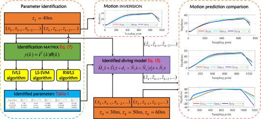
Fig.2 Block diagram of motion inversion and prediction. |
4.1. Description of a piston-driven profiling float prototype
Fig. 3 illustrates a piston-driven profiling float prototype used in the field tests, as detailed by Bai et al. [44]. The buoyancy system of the prototype consists of an aluminum tube, a linear actuator, a draw-line sensor, and a piston. The movement of the piston changes the buoyancy of the float, while the draw-line sensor measures the position of the piston as control feedback. Field tests were conducted in Qiandao Lake, located in Zhejiang Province, China, with a maximum depth of 100 m. For safety reasons, the maximum desired tracking depth was set to 60 m.
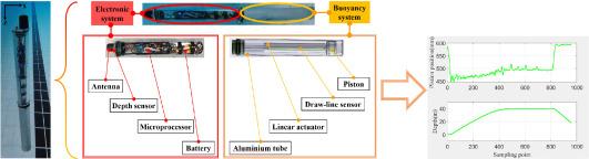
Fig.3 Model of the piston-driven profiling float. |
The field experiment cases included m, m, m, and m. To reflect the motion prediction ability of the IVLS algorithm in limited field experiment cases, the middle data set with m is used as the sampling data for parameter identification. Additionally, the field experiment datasets of , , and are used as validation data for motion prediction. The sampling frequency of the depth data is 1.43 Hz for m and 2.78 Hz for m. In addition, depth tracking was achieved using the proportional integral differential (PID) algorithm, which is a model-free controller. The curves in Fig. 2 show that the PID-based controller produced a large control signal when m. Due to the significant time lag effect of the piston-driven buoyancy system, sudden changes were not observed, and the float gradually reached the desired depth at a slow rate. As a result, the control signal asymptotically converged to zero. In order to increase the complexity of the input data, we modified to 0 m when the true depth curve had stabilized at 40 m, resulting in a trapezoidal true depth curve.
4.2. Diving dynamics identification and inversion
In order to obtain parameter identification results, the experimental data with m is used with Eq. (5) as the depth mechanism model. Table 1 shows the results obtained using different algorithms. A perceptive examination of these results reveals that the parameters derived using the LS-SVM and RWLS algorithms are significantly smaller than those obtained using the IVLS algorithm. Specifically, the value of is a only and for the LS-SVM and RWLS algorithms, respectively. Contrastingly, the IVLS algorithm yields a value of .
Table 1 Comparison of parameter identification results. |
| Algorithms | |||||
|---|---|---|---|---|---|
| IVLS | 3.95 | 0.489 | 0.0008 | 0.0021 | 0.1516 |
| LS-SVM | 0.0386 | 0.005 | 0.00000 | 0.00019 | 0.00049 |
| RWLS | 0.6430 | 0.1163 | 0.0002 | 0.0006 | 0.0029 |
The curves in Fig. 4(a) show the results of depth motion inversion obtained using the IVLS, LS-SVM, and RWLS algorithms. As depicted, all three algorithms provide a good fit to the actual curve. Fig. 4(b) shows the inversion error, offering a more vivid representation of the precision of the motion inversion across the three algorithms. In scenarios where the number of sample points is less than 800, each algorithm displays certain errors. The RWLS algorithm shows the most significant deviation, with the absolute value of the maximum error exceeding 6 m. Conversely, the LS-SVM algorithm has an absolute maximum error exceeding 4 m. The IVLS algorithm outperforms both, keeping the absolute value of the maximum error below 4 m, thus demonstrating superior accuracy in motion inversion in this scenario. As the number of sampling points approaches 800, notable fluctuations are observed in the piston position-transiting from approximately 500 mm to around 600 mm. Under these conditions, the inversion curve obtained by the IVLS algorithm (represented by the red curve) shows the best fit with the true curve. The absolute value of its error remains consistently below 4 m, while the error of the LS-SVM algorithm exceeds an absolute value of 6 m. This indicates that the parameter identification results of the IVLS algorithm better capture the motion dynamic characteristics of the float compared to the RWLS and LS-SVM algorithms.
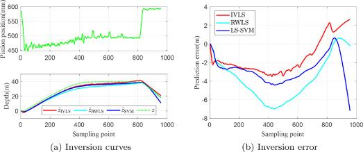
Fig.4 Motion inversion comparison with m. |
Remark 4: To optimize the performance of the algorithms, the penalty factor of the LS-SVM algorithm and the factors and of the IVLS algorithm are appropriately tuned using the trial-and-error method. The optimal value of , and is found to be 5.8731, 0.0005 and 4, respectively, which resulted in better motion inversion performance based on m, as shown in Fig. 4(a).
4.3. Diving motion prediction
For the diving prediction, field experiment datasets with 30 m, 50 m, and 60 m are used as control inputs and depth benchmarks. The performance of the LS-SVM, RWLS, and IVLS algorithms is then evaluated by using these datasets, as presented in Fig. 5, Fig. 6, Fig. 7.
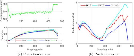
Fig.5 Motion prediciton comparison with m. |
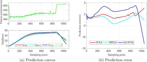
Fig.6 Motion prediciton comparison with m. |
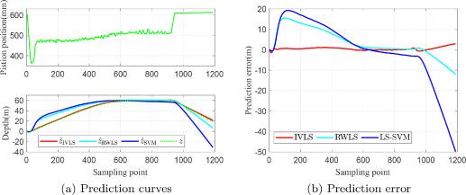
Fig.7 Motion prediciton comparison with m. |
Fig. 5 (a) displays the actual depth curve with 30 m and the corresponding prediction curves generated by the three algorithms. All three algorithms fit the actual depth curve to some extent, but Fig. 5(b) demonstrates that the IVLS algorithm yields smaller prediction errors overall.
For the data with 50 m, as shown in Fig. 6, the LS-SVM algorithm produces results with larger depth prediction errors, with the maximum depth error exceeding 10 m. In contrast, the RWLS algorithm exhibits better depth prediction performance, with the maximum depth error not exceeding 5 m. Moreover, the depth prediction curve based on IVLS shows the best fit with the actual curve, indicating that the IVLS algorithm better captures the motion characteristics of the vehicle when 50 m.
Fig. 7 presents the depth prediction performance of the three algorithms for 60 m. Under this dataset, the RWLS and LS-SVM algorithms exhibit larger depth prediction errors compared to the case of 50 m, with the maximum depth prediction error of the RWLS algorithm exceeding 10 m and that of the LS-SVM algorithm approaching 50 m. Conversely, the IVLS algorithm maintains excellent depth prediction performance for 60 m, with the maximum depth error being less than 2 m.
Based on the above analyzes, the IVLS algorithm exhibits superior generalization capabilities compared to both the RWLS and LS-SVM algorithms in terms of motion prediction based on parameter identification results. This enhanced performance of the IVLS algorithm is consistently demonstrated across datasets of varying depths. In each instance, whether at depths of , or , the IVLS algorithm's predictions have been shown to be markedly precise and reliable, as evidenced by the minimized prediction errors and the close fit of its output to the actual depth curves. In contrast, both the RWLS and LS-SVM algorithms show significant deviations and larger errors in their predictions, especially as depth increases. The results indicate the robust adaptability of the IVLS algorithm and confirms its effectiveness in capturing the intrinsic motion characteristics of the float at different operating depths.
Remark 5: In practice, the parameters of the diving model in Eq. (5) are typically fixed. Hence, the model-based motion prediction results for the verification cases with 30 m, 50 m, and 60 m rely on the identified parameters listed in Table 1, rather than undergoing a re-identification process.
4.4. Error metrics-based performance analysis
To provide a more intuitive representation of the performance of the three algorithms, Table 2 presents a comparative analysis of three parameter identification algorithms for the diving model of the piston-driven profiling float prototype. The performance of these algorithms is assessed using four error metrics, namely AVGAE, RMSE, [48], and MAXAE, over four different cases with varying desired depths of 30 m, 40 m, 50 m, and 60 m. A careful examination of the results leads to several important observations.
Table 2 Performance Metrics. |
| Cases | Algorithms | AVGAE (m) | RMSE (m) | MAXAE (m) | |
|---|---|---|---|---|---|
| m | IVLS | 1.756 | 2.077 | 0.950 | 3.822 |
| RWLS | 1.951 | 2.391 | 0.934 | 4.598 | |
| LS-SVM | 2.406 | 2.841 | 0.907 | 4.282 | |
| m | IVLS | 2.388 | 2.495 | 0.965 | 3.494 |
| RWLS | 4.653 | 4.962 | 0.860 | 6.972 | |
| LS-SVM | 3.097 | 3.220 | 0.941 | 7.064 | |
| m | IVLS | 1.024 | 1.145 | 0.995 | 2.259 |
| RWLS | 2.356 | 2.603 | 0.975 | 4.197 | |
| LS-SVM | 1.741 | 1.929 | 0.986 | 12.456 | |
| m | IVLS | 0.553 | 0.655 | 0.999 | 1.422 |
| RWLS | 7.256 | 8.950 | 0.802 | 15.547 | |
| LS-SVM | 8.782 | 11.117 | 0.695 | 19.222 |
First, the IVLS algorithm consistently outperforms the LS and LS-SVM algorithms in all cases in terms of AVGAE, RMSE, and MAXAE. The IVLS algorithm also demonstrates its superiority in terms of as well, with the highest values for all desired depths, indicating a better generalization ability. Therefore, the IVLS algorithm can reduce the effects of noise and uncertainties, resulting in more accurate parameter estimation.
Second, the performance of the LS and LS-SVM algorithms varies significantly across the different desired depths. Specifically, the LS algorithm performs relatively well at a desired depth of 30 m, with an AVGAE of 1.951 m and an of 0.934. However, its performance deteriorates as the desired depth increases, reaching an AVGAE of 7.256 m and an of 0.802 at a desired depth of 60 m. This decline in performance suggests that the LS algorithm may not be well suited to handle the complexities and uncertainties associated with larger desired depths. On the other hand, the LS-SVM algorithm shows relatively stable performance across the different desired depths, although its error metrics are consistently higher than those of the IVLS algorithm. The stable performance of the LS-SVM algorithm can be attributed to its ability to handle nonlinearities and uncertainties in the data due to its kernel-based approach.
Third, it is important to note that the performance gap between the algorithms becomes more pronounced as the desired depth increases. This observation underscores the importance of selecting an appropriate parameter identification algorithm for marine craft depth control systems, particularly when operating at larger depths. The choice of algorithm can significantly impact on the accuracy, reliability, and overall performance of the system.
In conclusion, this comprehensive and in-depth comparative analysis reveals that the IVLS algorithm is the most robust and accurate approach across all desired depths. The IVLS algorithm consistently outperforms the LS and LS-SVM algorithms in terms of AVGAE, RMSE, , and MAXAE, indicating a superior ability to generalize and fit the depth data. The findings suggest that the IVLS algorithm should be the preferred method for marine crafts' parameter identification, ensuring better accuracy and reliability in real-world applications.
5. Conclusions
In this paper, the IVLS algorithm is proposed for parameter identification and model-based prediction of marine crafts utilizing field data. Specifically targeting the piston-driven profiling float characterized by particular features, the diving model equation was decoupled from six degrees of freedom to one degree of freedom, enhancing model simplicity without compromising accuracy. To further optimize precision and minimize modeling error, a refined dynamics model was introduced, incorporating additional actuator nonlinear coefficients and discretized employing the first-order Euler method, laying a solid foundation for subsequent parameter identification. Acknowledging the limitations of the RWLS algorithm, particularly its inability to ensure convergence in scenarios polluted with noisy data, the IVLS algorithm was innovatively proposed. Its convergence was proved from a probabilistic perspective, marking a significant methodological breakthrough. The performance of the IVLS algorithm was validated through a series of diving tests datasets conducted in Qiandao Lake. Here, diving dynamics inversion, diving motion prediction, and an error metric-based performance analysis collectively highlighted the superior accuracy and generalization ability of the IVLS algorithm over four datasets when compared to the LS-SVM and RWLS algorithms. Notably, the IVLS algorithm achieved a MAXAE of less than 1.5 m for = 60 m. Hence, the IVLS algorithm stands out as a robust and accurate approach for parameter identification and diving motion prediction for marine crafts.
Considering that the model herein is a single degree of freedom, our future work will focus on the coupling effect between different degrees of freedom. Discussing potential applications, this paper could substantially benefit marine science research and explorations. By offering a more accurate and noise-resistant motion prediction, it enhances the quality of data collection in marine environments, facilitating improved analysis and understanding of marine ecosystems, ocean currents, and underwater geological structures. The improved accuracy and robustness in the motion predictions of marine crafts could support more precise deployment of scientific instruments and sampling equipment in oceanographic studies. Thus, the advancements proposed in this paper could play a crucial role in augmenting the capabilities of marine scientific research and exploration efforts, promoting a richer understanding of our oceans.
Declaration of Competing Interest
The authors declare that they have no known competing financial interests or personal relationships that could have appeared to influence the work reported in this paper.
