
1. Introduction
One of the main problems in oceanography is the study of inward waves dynamics [1] as a specific model of physical movements that occurs within fluids. The results of these studies are directly related to the issue of maritime transport, instantaneous motion and energy, as well as to the navy and engineering. The mathematical modeling of dynamics of inward waves in ocean leads to various forms of nonlinear evolution equations (NLEEs). Historically, the famous KdV equation was the first model developed by Korteweg and De Vries to explain the diffusion of low-amplitude inward waves in shallow water [2], [3]; however, this equation for long-amplitude inward waves will not be practical. To overcome this deficiency, especially for deep sea inward waves, Benjamin [4] and Ono [5] obtained Benjamin-Ono equation. In [6], Kubota et al. presented the intermediate long wave (ILW) equation for propagating weak nonlinear inward waves in stratified fluids of limited depth. In [7], Choi and Camassa obtained a form of equation that controls the evolution of inward waves at the interface between two immiscible inviscid fluids. However, in order to more accurately model the inner ocean waves in terms of two-layer stratification, [8] Song et al. proposed the Schrödinger nonlinear equation (NLSE), and as a result, the interaction of the two could be formulated by coupled NLSE. Therefore, finding accurate NLSE solutions and their coupled models will have a significant impact on the behavior of inward ocean waves and their interactions, respectively. It can be said that the solutions of these equations give more insight into the physical aspects of oceanic inward waves as well as the designated ocean science problems.
On the other hand, a great result that eliminates the divergence and propagation of radiative wave conduction is the nonlinear change in the refractive index of the medium, which is associated with the propagation of a strong electromagnetic wave. Due to the nonlinear change in the refractive index of the medium, it is possible to have wave packets in which the propagation of the wave occurs without any deformation in the wave envelop and are stationary in time [9]. Various people have worked on this type of phenomenon, such as Zakharov and Shabbat [10], who have proposed a theory for waves of the same polarity everywhere in two-dimensional geometry. The following two items can be considered as main features of their work:
a) A part of entered radiation to the medium is divided to a certain number of channels;
b) Each channel has a definite direction and their intensity decreases exponentially with increasing distance from its axis.
Manakov in [9] generalized the theory of proposed by Zhakharov and Shabat [10] to the case of waves of arbitrary polarization. He showed that when a wave with varying polarization enter into the nonlinear medium, it is separate into various beams with radiations of constant polarization. This case is known as polarization filter. An important result that Markov achieved in [9] relates to self-focused two-dimensional waves due to the one-dimensional self-modulation of the electromagnetic wave with arbitrary polarization. During the collision of latter waves, their velocities and amplitudes remained unchanged, but their polarizations do changed. Consequently, the mentioned electromagnetic waves can be considered as a soliton.
The mathematical modeling of the above statements phenomena was done by Manakov in [9] as an integrable coupled NLSE of Manakov type
where and are slowly varying envelops of the two interacting polarized waves and and , are positive parameters. The term rogue or freak wave has long been used in marine science for waves that are much high and deeper than would be expected for the sea state [11]. Rogue waves detected only seconds before strike a ship, which can be seen in both shallow waters and oceans, are very dangerous [12]. These waves occur not only in the oceans [13], but also in the atmosphere [14], optics [15] and so on. The dynamics of rogue waves are well formulated by the NLSE. One of these models is the Manakov model of coupled NLS equation. Many studies have been done on rogue waves for this equation [16], [17], [18], [19].
Various effective approaches for obtaining exact solution of equations arising from modeling real-world problems have been successfully applied by scientists in recent years [20], [21], [22], [23], [24], [25], [26], [27], [28], [29], [30], [31], [32], [33], [34], [35], [36], [37], [38], [39], [40], [41], [42], [43], [44], [45], [46], [47], [48], [49], [50], [51], [52], [53]. These methods are also applied for finding the solitary wave solutions of system (1). Due to the balance between nonlinearity and dispersion, solitary wave solutions are stable localized waves that propagate without amplitude attenuation and deformation in a nonlinear environment [54], [55]. In the study [56], it was revealed that the peak of a solitary wave is weakly affected by the unsmooth boundary. The control of energy exchange of Manakov vector-soliton collision is studied in [57]. Radhakrishnan and Lakshmanan using the results of Painleve analysis obtained the bright and dark N-soliton solutions of the Manakov model (1) in [58]. In [59] Buryak et. al studied the interaction between dark and bright solitary wave solutions of model (1). In addition, by considering the analytical solution of the system (1), in [60], Balancer and Pare investigated some conditions for soliton switching and energy coupling in the case of equal cross- and self-phase modulation effects. Recently, in [61], [62], Yildirim applied the experimental equation method and the modified simple equation method, respectively, to obtain the soliton optical molecules of Manakov model (1).
In this paper, our first interest is applying the extended auxiliary equation (EAE) and -expansion methods to emphasis its power in treatment nonlinear equations. These methods can be implemented on many of nonlinear models with various types of nonlinearity. The next interest is in the determination of solitary wave solutions of Manakov model (1) using present methods. These powerful and efficient methods have not been applied before to obtain the model solutions we study in this article.
2. Governing equation
with the wave transformation
where are the phase and amplitude component functions,respectively. In the last equation, the parameter describes the soliton frequency, is its wave number while is the phase center. Substituting Eq. (3) into Eq. (2), for and , the imaginary equation is as follows:
and the real part is as follows:
With , above equation is collapsed into
By balancing and , the balance number can be found.
3. Mathematical analysis of the Manakov model
3.1. The solution of Eq. (1.1) using the EAE method
We will use the EAE method to solve Eq. (2). With the effect of balancing principle applied to Eq. (7), we have
Inserting Eq. (8) into Eq. (7) and equating all the coefficients of same power of to zero, respectively, we have
Above Eqs. (9) yield the following set of coefficients for the solutions.
From (10) and (4), we obtain that Eq. (2) has the Jacobi elliptic function (JEF) solutions:
or
where
From (10) and (4), the JEF solutions are
or
where .
From (10) and (4) we conclude that Eq. (2) possess the JEF solutions:
or
where .
From (10) and (4), the solutions of Eq. (2) are
or
where .
From (10) and (4), the solutions are:
or
where .
From (10) and (4), solutions of Eq. (2) are:
or
where .
3.2. The solution of Eq. (1.1) using the -expansion method
In this section, the -expansion method is used to get the solutions of Eq. (2). Using homogeneous principle, balancing and , we have , . Therefore, the solution can be given as
where , is constant. By placing Eq. (35) and its derivatives in Eq. (7), and also by setting the different power factors of equal to zero, we will have:
The algebraic equations system gives the following set of coefficients for the solutions:
From (37) and (4), the solution is obtained as follows:
From (37) and (4), we obtain
From (37) and (4), we get,
From (37) and (4), we get,
From (37) and (4), the solutions are
4. Graphical demonstration
To find exact solutions to the governing equations, we successfully used and the developed auxiliary equation methods. Our figures show 3D surface diagrams and 2D-contour graphics show the obtained solutions. In this study, a variety of traveling waves solutions, periodic-like solutions, soliton-like solution are obtained through the trigonometric and exponential solutions.
5. Conclusion
In this paper, we find the new solutions of the Jacobi elliptic equation and the exact solutions of Eq. (2). In the present article, using the EAE method and the -expansion method, we have obtained. With the help of Maple, the methods applied in this paper provide a powerful mathematical tool for finding accurate general solutions to a large number of NLPDEs or NLSEs in mathematical physics. To obtain Manakov model optical solitons, experimental equations and simple modified equations have been applied in [61], [62]. The methods applied in this paper provide additional new solutions in addition to the solutions obtained by the experimental equation and the modified simple equation methods, and also, in theory, to accurately select the parameters, some of our solutions coincides with the solutions available in [61], [62]. Moreover, we plotted 3D and 2D plots for some of our obtained solutions for more dynamical properties. We get three forms of solitary wave solutions and Figs. 1, 2, 3, 4, 5, 6, 7, 8, 9, 10, 11, 12, 13, 14, 15, 16, 17, 18, 19, 20 show that very obviously for these models. Fig. 5, Fig. 6, Fig. 13, Fig. 14 and 18 present multi-soliton solutions. Figs. 9 and 10 demonstrate rational function solutions. Fig. 17 shows single soliton solutions. As known, solitary waves and solitons are the specic types of localized solutions of several nonlinear physical models. By substituting the results within the original equation, we show that all solutions enrich the original equation. We wish this paper to contribute to future research and have different applications in the fields of modern optics and engineering.

Fig.1 Profile of (38) for , , |
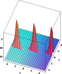
Fig.2 Profile of (39) for , , |
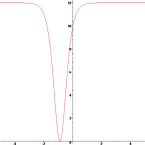
Fig.3 2D-profile of (38) for , within |

Fig.4 2D-profile of (39) for , within |
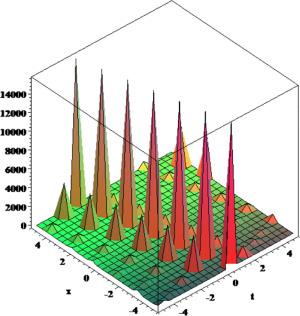
Fig.5 Profile of (40) for , , |
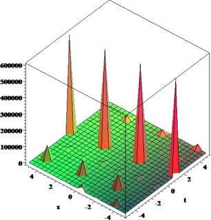
Fig.6 Profile of (41) for , , |
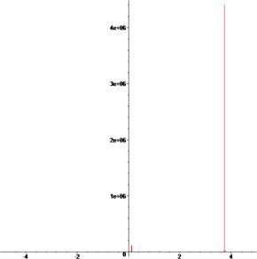
Fig.7 2D-profile of (40) for , within |
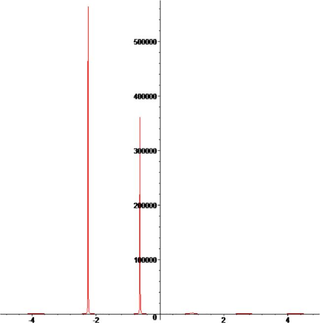
Fig.8 2D-profile of (41) for , within |
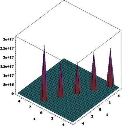
Fig.9 Profile of (42) for , , . |
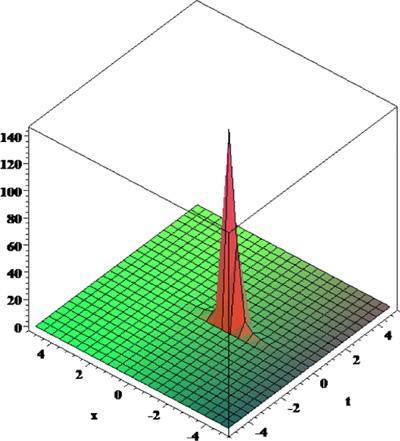
Fig.10 Profile of (43) for , , |
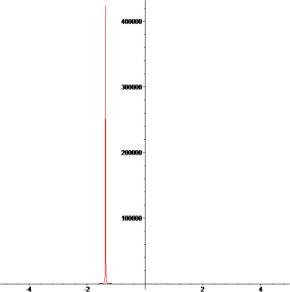
Fig.11 2D-profile of (42) for , within . |
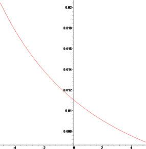
Fig.12 2D-profile of (43) for , within . |
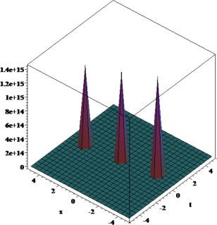
Fig.13 Profile of (44) for , , |
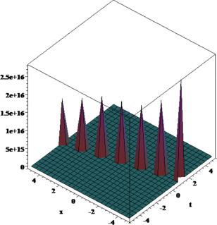
Fig.14 Profile of (45) for , , |
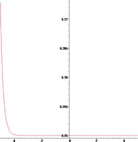
Fig.15 2D-profile of (44) for , within |
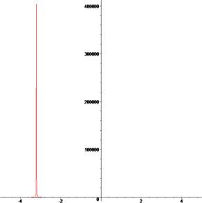
Fig.16 2D-profile of (45) for , within |
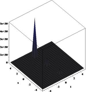
Fig.17 Profile of (46) for , , . |
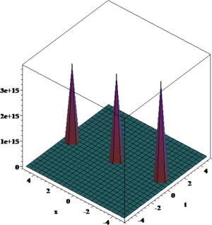
Fig.18 Profile of (47) for , , . |
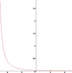
Fig.19 2D-profile of (46) for , within . |
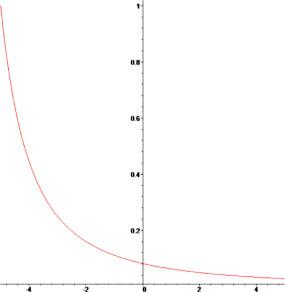
Fig.20 2D-profile of (47) for , within . |
Declaration of Competing Interest
The authors declare that they have no known competing financial interests or personal relationships that could have appeared to influence the work reported in this paper.
