
1. Introduction
The interaction between ships and sea ice is a complex and dynamic process, with level ice and floating ice being the main ice conditions encountered by vessels during navigation in ice areas [1,2]. With the opening of the Arctic Channel, polar ships will inevitably navigate through level ice and floating ice conditions. Ice loads at any given time will vary with ice conditions, where ships navigating on continuous level ice will encounter higher resistance. However, ice load is an important evaluation result of ship-ice collisions and an important transient excitation of ice-induced vibration, which directly affects the calculation results of ship-ice collision-induced vibration [3⇓⇓⇓-7]. Therefore, the study of numerical analysis methods for ship-ice collision-induced vibration problems is essential for the analysis of both ship-ice collision and transient vibration.
For the numerical calculation methods of ship-ice collision-induced vibrations, researchers have only considered the effects of the attached water mass and ignored hydrodynamic loads in the early stages of the ship-ice collision problem. Kim [8] simulated a continuous ship-level ice collision using the attached water mass method and investigated the effects of different speeds and ice thicknesses on the ice load. Kwak [9] analyzed the structural strength and ice mechanical properties of ship-ice collisions through the constantly added mass method to MS_DYTRAN and compared them with the experimental data. Tian [10] calculated and analyzed the constantly added mass model in ship-bridge collision simulation. Pedersen [11] evaluated the effect of water using the constantly added mass method. Then, the energy losses of ship-ship collisions and ship-platform collisions were studied by an analytical method and compared with the energy losses of time-domain simulations. Yamada [12] analyzed the force and energy during a ship-ship collision that used the same process as Pedersen and compared it with the force and energy obtained from FEA. However, the constantly added mass method tends to ignore the effects of fluid resistance and object buoyancy, which affects the accuracy of ice load prediction. Therefore, two methods have been proposed for buoyancy simplification and fluid-structure coupling as researchers gradually consider the influence of fluid. Liu [13] simulated the ship-ice interaction process by introducing near-field dynamics to calculate ice loads without considering the gravity and buoyancy of the ice. Lubbad [14] simplified the buoyancy of level ice in a spring distribution at the bottom of the level ice. Wang [15] used LS_DYNA software to simulate the interaction of slope marine structures with level ice, but only the initial part of the ice-structure interaction was simulated. NI [16] considered the effect of fluids on ship-ice interactions using a fluid-structure coupling method. The validity and reliability of the simulation were determined by comparing numerical results with empirical formulations and comparing the longitudinal, lateral, and vertical ice resistance of the vessel with and without fluid conditions. Song [17] compared the results of the fluid-structure coupling method, the constantly added mass method, and an experimental method for collisions between ice and floating structures in LS_DYNA. It was found that there is a difference between the fluid-structure coupling method and the constantly added mass method due to the effects of bow waves. According to the comparison of the experimental method, the fluid-structure coupling method can better simulate the real collision process. Other researchers [18⇓-20] have carried out measurements and analyses of ice-induced vibrations on icebreakers to study the vibration comfort of full-scale ships. Wen [21] used the virtual modal method to calculate the transient noise analysis of a ship undergoing an ice floe collision, but it assumed the collision force as a triangular force and did not use the actual ice load. It can be seen in the above research that the constantly added mass method and fluid-structure interaction method are mainly used in the study of ship-ice collisions. Among them, the constantly added mass method considers the mass of the attached water, which has the advantages of a small calculation scale and fast calculation speed. However, because the fluid is not considered, the time of the peak in the early calculation results will be shifted forward, and the later peak will be significantly larger [22⇓⇓-25]. Compared with the constantly added mass method, the fluid-structure interaction method has greater advantages. It can consider the influence of fluid resistance and obtain more accurate results. However, its disadvantage is that the calculation scale is obviously greater than the constantly added mass method, and it is difficult to simulate ship-ice collisions with level ice scales reaching 100 m or more. Researchers have mostly used ship-ice-water coupling when using the fluid-structure interaction method to analyze ship-ice collisions and have ignored air coupling. Although the ship-ice-water coupling method considers the fluid influence and improves the calculation accuracy, its disadvantage is that the buoyancy of the object cannot be considered [16,17]. The ship-ice-water‒air coupling method cannot only consider the fluid influence but also apply the correct buoyancy and reduce the calculation scale on the basis of the S-ALE algorithm. This is of great significance to the analysis of ship-ice collision-induced vibration. At present, there are few numerical analysis studies on the ship-ice collision-induced vibration response. Some numerical studies have simplified the ice load and water as triangular forces and constantly added mass but have not achieved accurate vibration prediction. Consequently, it is necessary to solve the ship-ice-water‒air full coupling problem, improve the calculation accuracy and reduce the difficulty of calculating large-scale fluid-structure interactions.
To assess the element sizes and model ranges of ship-ice collision-induced vibrations, Lu [26] simulated the interactions between slope structures and level ice using the cohesive element method. To achieve convergence of the results, cross-triangular meshes were created to simulate level ice, and various methods were used to reduce the mesh dependence, such as creating unstructured meshes and using a penalty method to obtain the initial stiffness of the cohesive elements. The model only considered type I fractures and ignored locally broken ice, which meant that level ice could only break in the bending damage mode. Wang [15] established a model to simulate the preliminary stage of ice-structure interaction and conducted a comparative analysis of cross-triangular and quadrilateral meshes by considering local broken and bending failure based on LU. Element sizes and modeling ranges of the level ice were not specified. Kim [27] directly assumed a longitudinal mesh size of 500 mm and a modeling range of 100×100 m for level ice in simulations of the interaction between a ship and level ice, without illustrating the basis for the choice of size. Ni [16] used an element size of 1 × 1 × 1 m and a modeling width of 15 times the ship width for level ice in a simulation of the interaction between a ship and level ice. Based on Lau [28], Zhang [29] simulated the ice-breaking process of the ARAON icebreaker. The length of level ice was 2.2 times the ship length, and the width was 10 times the ship width. However, the influence of water was not considered in the simulation process. This resulted in an easy increase in the modeling range without the convergence of the element size. Zhang [30] established a model of water that used the fluid-structure interaction method. Although the effect of fluid resistance was considered, the atmospheric pressure over the fluid field was ignored, and the influence of the gravity field on the floating state during ship-ice collision was not considered. This still affected the accuracy of the ice load prediction. In addition, many studies of grounding and collisions have been analyzed with relatively coarse finite element meshes or finite meshes, which leaves uncertainties in the accuracy of the analysis of the problem. Ideally, finite element models should be as accurate and detailed as possible to capture regional folding and instability effects, but this requires excessive computational time and resources. On the other hand, a coarse mesh can satisfy the requirements for computational efficiency but not for accuracy. However, inappropriate ship and ice element sizes can adversely impact the calculation results, especially the prediction of changes in collision forces and plastic changes in the hull structure; inappropriate element sizes of the fluid field can produce errors in the floating state of objects on the water surface and cannot ensure that objects float reasonably well [31⇓-33]. Therefore, there should be a uniform model range of level ice and element sizes that allows the load to converge for the numerical simulation of a ship-ice-water‒air coupling collision.
In summary, it is necessary to investigate the full coupling method, meshing sizes, and modeling ranges involved in ship-ice collision-induced vibration analysis. This paper investigates the method of ship-ice-water‒air full coupling and the coupling setup in ship-ice collisions and ice-induced vibrations. On this basis, this paper determines the element sizes of the ship, level ice, water, and air and the modeling ranges of the level ice, water, and air in the ship-ice-water‒air coupled collision analysis. Meanwhile, the mesh sizes and division ranges of the gradient meshing model of the ship and the modeling ranges of the fluid field are also determined in the ship-water‒air coupled vibration analysis. A method for transforming level ice into ice load is given. Based on the full ship-ice-water‒air coupling, the S-ALE algorithm is introduced and compared with the traditional ALE algorithm in terms of computational efficiency.
2. Concurrent analysis of ship-ice collision-induced vibration of the polar transport vessel
2.1. Target model of the polar transport vessel
In this paper, a polar transport vessel is taken as the target object to study the meshing generation and modeling region in a numerical analysis of ship-ice collision-induced vibration. The finite element model of a polar transport vessel is shown in Fig. 1, and the main dimension parameters are shown in Table 1.
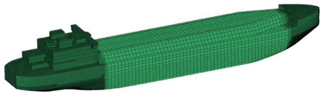
Fig. 1. Finite element model of a polar transport vessel. |
Table 1. Main dimensions of the model. |
| Ship prototype | Length | Breadth | depth | draught | Displacement |
|---|---|---|---|---|---|
| Value | 300.0m | 50.0m | 26.5m | 11.7m | 130,202.0t |
2.2. Ideal concurrent analysis of ship-ice collision-induced vibration
For the ship-ice collision problem, three kinds of models are selected: the rigid model, the rigid-elastoplastic hybrid model, and the elastic‒plastic model. The most ideal model is the elastic‒plastic model, which can be used to study both the external dynamics and internal dynamics of ship-ice-water‒air coupling collisions, as shown in Fig. 2. However, its calculation scale is too large for the existing calculation method of fluid-structure interaction to complete this part of the research. Therefore, most researchers have used the rigid model in the early stages of ship-ice collision studies considering the effect of fluid, as shown in Fig. 3. However, this can only be used for the analysis of external dynamics, thus omitting the internal dynamics of the structure. Research on internal dynamics is a non-negligible part of predicting the safety of a hull structure. As a result, with the rapid development of computer technology, researchers are more inclined to use semi-rigid-elastoplastic models, which can consider both the external dynamics of the hull structure and the internal dynamics of the collision region, as shown in Fig. 4.
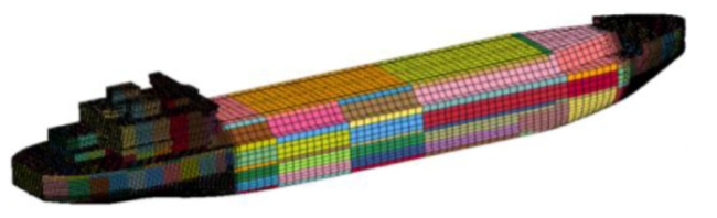
Fig. 2. The ship model consists of elastic‒plastic material. |
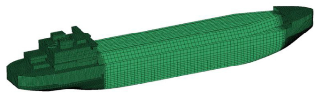
Fig. 3. The ship model consists of rigid material. |
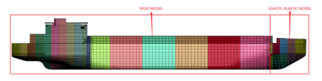
Fig. 4. The ship model consists of rigid and elastoplastic material. |
For the ice-induced vibration problem, the superstructure and stern vibration response are important concerns. The response in these regions cannot be predicted if the rigid and semi-rigid-elastoplastic models are used, so the elastic‒plastic model is the only choice, as shown in Fig. 2.
When performing a numerical analysis of ship-ice collision-induced vibration, the ideal method used for a ship is an elastoplastic model for numerical calculations of coupled ship-ice-water‒air collisions. After the calculation is completed, the collision force curve and structural vibration response are output simultaneously to achieve the simultaneous analysis of ship-ice collision and vibration response. The specific process of numerical analysis is shown in Fig. 5. The ship-ice-water‒air coupling setting mainly considers the resistance and buoyancy of the fluid. It can include both ship-ice interaction and fluid-structure interaction to improve the calculation accuracy of fluid-structure interaction. However, this method is too large in computational scale and is currently difficult to implement.
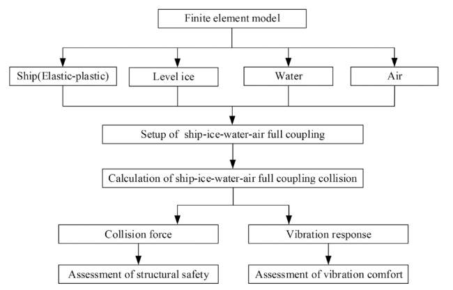
Fig. 5. Ideal numerical analysis procedure for ship-ice collision-induced vibration. |
2.3. Simplified numerical analysis of ship-ice collision-induced vibration
To effectively investigate the vibration response regulation during the ice-breaking process, a reliable and effective method is needed. In this paper, the ship-ice collision and vibration response are calculated separately based on the ideal analysis method of ship-ice collision-induced vibration. The specific process of numerical analysis is shown in Fig. 6. First, a ship-ice-water‒air coupled collision calculation is carried out to obtain ice load data. The ice load is then applied as a transient excitation source for the elastoplastic ship model to obtain a reliable vibration response of the ship structure. In the simulation of ship-ice-water‒air coupled collision, it is necessary to consider the coupling effects of four media: the ship, level ice, water, and air, which includes ship-ice interactions and fluid-structure interactions. The influence of fluid resistance and gravity field on the floating state of water objects can be considered simultaneously to achieve more accurate ice load prediction and improve the accuracy of ship-ice collision calculation. In the simulation of vibration analysis, it is necessary to consider the coupling effect of three media—the ship, water, and air—simultaneously. The coupling of the three is to consider the fluid-structure interaction, while the transformation of the level ice into ice loads is to consider the ship-ice interaction.

Fig. 6. Simplified numerical analysis procedure for ship-ice collision-induced vibrations. |
2.4. Ship-ice-water-air four-phase coupling algorithm
The process of the ship-ice-water‒air four-phase coupling algorithm is shown in Fig. 7. The core settings are mainly in the ambient boundary, hydrostatic pressure, gravity field, and coupling settings. The ambient boundary is used to allow for the inflow and outflow of fluid by using local pressure gradient changes on the boundary, which in turn defines the boundary conditions of the infinite field of the fluid. To eliminate the effect of the initial wave on the ship-ice collision, the air pressure is achieved to one atmosphere, and the water pressure varies with water depth by applying hydrostatic pressure to the fluid field. A gravity field is applied globally through the gravity keyword. Then, air is inserted where the ship and water, level ice and water overlap when considering a reasonable floating state of objects. Finally, the four-phase ship-ice-water‒air coupling is realized by applying keywords such as coupling and contact. The ship-ice-water‒air coupling method can achieve a more accurate prediction of ice loads and vibration response while considering the effects of both fluid and buoyancy and improving the calculation accuracy of the ship-ice-water‒air coupled collision and vibration. If these factors are not considered, a good simulation of the initial state and interaction between the ship and ice in the water cannot be assured, which will also directly affect the accuracy of the ice load and vibration response prediction.

Fig. 7. Four-phase ship-ice-water‒air coupling process. |
3. Modeling method of collision analysis based on ship-ice-water-air full coupling
The accuracy of the calculation results must be guaranteed in the ship-ice-water‒air coupling collision problem, but the use of all fine elements will increase the computational effort. The problem should be divided into different units for the collision and non-collision regions due to the obvious locality of ship-ice collision. The collision region should be divided into fine elements to improve computational accuracy, while the non-collision region should be divided into asymptotic elements to improve computational efficiency. The element size of the collision region is mainly determined in the ship-ice-water‒air coupling collision model, and the division schematic is shown in Fig. 8.

Fig. 8. Schematic diagram of the meshing of the ship-ice-water‒air coupling collision model. |
The element size of the collision region is calculated by the convergence factor formula, as shown in Eq. (1). First, three element sizes—dense, medium, and coarse—are selected to calculate the ice resistance. Then, the convergence coefficient (RM) between different element sizes is calculated by the convergence factor formula to determine the load convergence. This indicates that the collision force shows monotonic convergence when RM ranges from 0 to 1 [15].
$ \begin{array}{l} R_{M}=\frac{\varepsilon_{\mathrm{md}}}{\varepsilon_{\mathrm{cm}}} \\ \varepsilon_{\mathrm{md}}=F_{M\mathrm{m}}-F_{M\mathrm{d}} \\ \varepsilon_{\mathrm{cm}}=F_{M\mathrm{c}}-F_{M\mathrm{m}} \end{array}$
where FMm is the ice resistance of the fine element, FMd is the ice resistance of the medium element, and FMc is the ice resistance of the coarse element.
3.1. Modeling method of ship structure
A ship-ice collision has obvious local characteristics. When meshing the hull structure, a distinction should be made between the collision and non-collision regions, where the mesh size of the collision region is sensitive to the calculation results. Mesh refinement of the region to be contacted is required to study the structural damage in the collision region and the overall collision load. Meanwhile, the non-collision region needs to be coarsened to reduce the computational efficiency and avoid generating too much computational scale, as shown in Fig. 9.

Fig. 9. Schematic diagram for meshing the ship model. |
Time step integration is a characteristic of the finite element technique, and each step of the calculation is required to satisfy the Courant criterion [30]. When the hull structure is a rigid material, the element size of the hull structure does not need to be too fine but only needs to ensure that the collision will not penetrate. When the hull structure is a model of elastoplastic or semi-rigid-elastoplastic material, the element size of the hull structure is approximately 250 mm according to the research of domestic and foreign researchers [30]. This element size can guarantee computational accuracy when calculating ship-ice collisions using the elastoplastic hull structure and improve computational efficiency.
3.2. Modeling method of level ice
The material (*MAT_ISOTROPIC_ELASTIC_FAILURE) in LS_DYNA is used to simulate level ice. The material is an isotropic elastic fracture failure model with a plastic strain failure criterion. When the effective plastic strain reaches the failure strain or the pressure reaches the failure of the cut-off pressure, the element loses its ability to bear stress [34,35]. The material parameters are shown in Table 2.
Table 2. Parameters of level ice material [35]. |
| Ice parameters | value |
|---|---|
| Ice density (kg/m3) | 910 |
| Young's modulus (GPa) | 2.2 |
| Yield stress (MPa) | 2.12 |
| Plastic hardening modulus (GPa) | 4.26 |
| The bulk modulus (GPa) | 5.26 |
| Plastic failure strain | 0.35 |
| Pressure (MPa) | −2 |
Since the size of the level ice element has a very important influence on the ice load prediction, it is necessary to analyze the convergence of the element size of the level ice before the formal calculation of ship-ice collision conditions. To better verify the applicability of the element size of level ice, the convergence of different element sizes in the collision region of the ship model is analyzed. Three element sizes of M1 = 1 m, M2 = 0.5 m, and M3 = 0.25 m are selected as the element sizes of the collision region of the level ice model, as shown in Fig. 10 (hidden fluid field).

Fig. 10. Finite element model of ship-ice-water‒air coupled collision based on the ship model. |
Ship-ice-water‒air coupled collision simulations are performed for the ship model based on three element sizes. Ice resistance values under different element sizes are calculated from the obtained ship-ice collision force curves. The convergence coefficient RM under the ship model is calculated according to Eq. (1) and is used as an investigating factor for the convergence analysis. The collision force curves under different element sizes are shown in Fig. 11, and the ice resistance values are shown in Table 3. The convergence factor for the ship model is RM = 0.267853 (0 < RM < 1). It can be observed that the convergence factors range from 0 to 1, which indicates that ice resistance shows monotonic convergence. Factors such as computational time and computational accuracy in the numerical analysis were considered comprehensively according to the number of elements and ice resistance. Therefore, M2=0.50 m is selected as the element size of the level ice in the collision simulation of the ship model in the collision region, which can obtain better ice load results and improve computational efficiency.
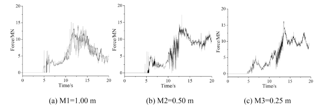
Fig. 11. Collision force curve based on the ship model. |
Table 3. The data on ice resistance. |
| Item | M1 | M2 | M3 |
|---|---|---|---|
| Element size of the level ice(m) | 1.00 | 0.50 | 0.25 |
| Element number of the level ice | 58,464 | 153,714 | 479,216 |
| Ice resistance(MN) | 4.456734 | 4.947694 | 5.079199 |
Level ice mainly experiences extrusion, bending, shear, and other forms of damage when the level ice collides with the inclined structure. The kinetic energy received by the level ice will be dispersed in different directions. For the ship model, the calculation conditions were determined by setting up a level ice model with different widths and lengths, as shown in Table 4. Based on the calculation working conditions, an impulsive ice-breaking calculation model is established to analyze the kinetic energy change of the level ice after the collision (i.e., the convergence of the longitudinal displacement results) to obtain the level ice range that can be directly applied to the ice-breaking calculation of the ship model. Considering the element size, the distance between the ship model and the level ice is set to 0.01 m, the initial velocity of the ship model is 2.5 kN (1.286 m/s), and the calculation time is set to 20 s. The finite element model of the ship-ice-water‒air coupled collision for Condition 1 is shown in Fig. 12.
Table 4. Calculated working conditions of the ship model. |
| Condition | Level ice width/m | Level ice length/m | Level ice thickness/m |
|---|---|---|---|
| 1 | 250(5B) | 150 | 1.5 |
| 2 | 300(6B) | ||
| 3 | 350(7B) | ||
| 4 | 400(8B) | ||
| 5 | 450(9B) | ||
| 6 | 500(10B) | ||
| 7 | 250 | 150(0.5L) | |
| 8 | 200 | ||
| 9 | 250 | ||
| 10 | 300(1L) | ||
| 11 | 350 | ||
| 12 | 400 |

Fig. 12. Finite element model of ship-ice-water‒air coupled collision (Condition 6). |
The ice-breaking simulation was carried out for the conditions in Table 4, and the changes in the longitudinal displacement (x-direction) of the level ice were obtained during the collision between the ship and the level ice, as shown in Figs. 13 and 14. The longitudinal displacement of level ice gradually decreases and converges as the width and length of level ice increase. For the simulation of the coupling collision between the ship model and level ice, the longitudinal displacement value tends to be stable when the level ice width reaches 300 m (6 times the ship width), and the longitudinal displacement value also tends to be stable when the level ice length reaches 300 m (1 time the ship length). Consequently, 300 m (width) × 300 m (length) can be chosen as the model range of the level ice, which is equivalent to 6 times the ship width and 1 times the ship length.
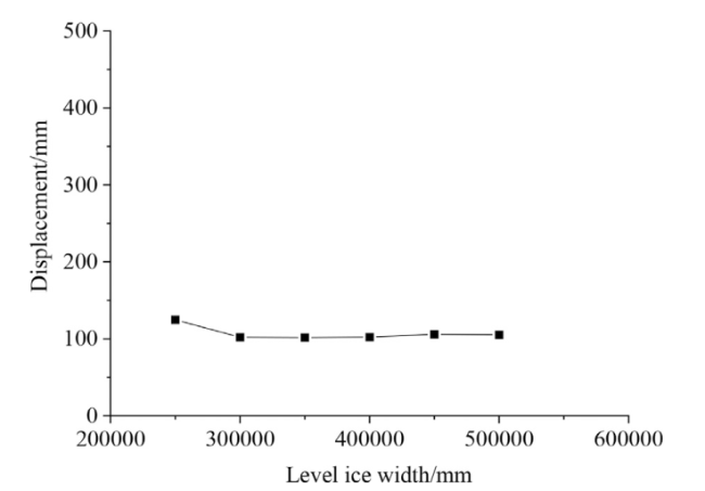
Fig. 13. The width-displacement curve of level ice. |
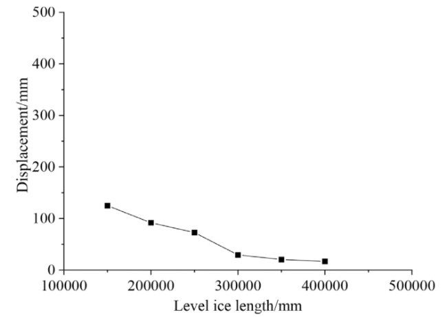
Fig. 14. The length-displacement curve of level ice. |
3.3. Modeling method of air and water
Table 5. Fluid material parameters. |
| Item | Water | Air |
|---|---|---|
| Density(kg/m3) | 1025 | 1.25 |
| Viscosity(N s/m2) | 8.684×10⁻⁴ | 1.764×10⁻⁵ |
| Pressure cutoff(Pa) | −10 | −1 |
| C0 | 101,325 | 0 |
| C1 | 2.25×10⁹ | 0 |
| C2 | 0 | 0 |
| C3 | 0 | 0 |
| C4 | 0 | 0.4 |
| C5 | 0 | 0.4 |
| C6 | 0 | 0 |
| E0(Pa) | 0 | 2.533×10⁵ |
| V0 | 1 | 1 |
The incorrect buoyancy will directly affect the ice load since the fluid field element size will affect the floating state of the structure. Therefore, it is important to choose a reasonable fluid field element size relative to the surface object. In this paper, we establish a finite element model of a rectangular shell, let it free-fall from an aerial position, and observe its vertical displacement and vertical velocity change. This is used to determine a reasonable fluid element size in the collision region [23]. The geometry of the rectangular shell finite element model is 20×5 × 5 m with a thickness of 0.1 m. The structure is made of No. 45 steel. The element size is 0.5 m, which is equivalent to the element size for level ice convergence when breaking ice on a ship. The bottom of the structure is 0.01 m from the water surface. The geometry of the fluid field finite element model is 60×30×30 m, in which the water geometry is 60×30×20 m and the air geometry is 60×30×10 m. The element size of the fluid field model is 1 m. The total number of elements is 63,304, and the total number of nodes is 68,330 in the finite element model, as shown in Fig. 15. The fluid field is set around the ambient boundary, and the fluid field is initialized with hydrostatic pressure, as shown in Fig. 16.
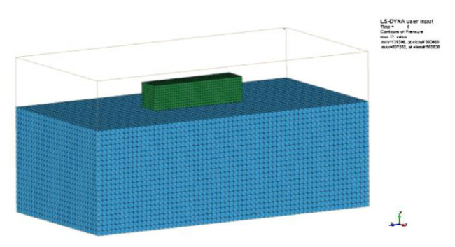
Fig. 15. Finite element model. |
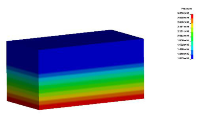
Fig. 16. Hydrostatic pressure initialization model. |
The variation in vertical displacement is shown in Fig. 17. The simulated draught value of the rectangular shell is approximately 3.643 m, and the theoretical draught value of the rectangular shell is 3.446 m according to the gravity-buoyancy balanced relationship. By comparing the theoretical and numerical solutions of the draught, this error can be accepted because the object is always undulating in the water and there is no sinking phenomenon. This can correctly simulate the floating motion of the real ship model with the combination of a 1 × 1 × 1 m element size for the fluid field and a 0.5 × 0.5 × 0.5 m element size for the level ice.

Fig. 17. Vertical displacement curve. |
For the ship-ice-water‒air coupling collision problem, the fluid mainly plays the role of interaction. Water is given priority, and the airfield only needs to maintain normal atmospheric pressure. The effect of the fluid field on the structure can be guaranteed when the buoyancy of objects such as ships is correct. Therefore, the fluid field can be useful only if the infinite field boundary condition is satisfied and does not lead to a decrease or absence of buoyancy. To verify the change in buoyancy with the height of the water, this paper modifies the height of the water to 2 times, 3 times, and 5 times the ship depth to observe the change in the object draught based on Fig. 15. The vertical displacement curve is given in Fig. 18, and the draught values are shown in Table 6. The results show that the simulated draught value will have a small fluctuation with the change in the fluid field dimension. However, the overall difference is not that large, and it is closer to the theoretical draft value. The vertical scale of the fluid field will not affect the floating state of the object, while the horizontal scale only needs to accommodate the ship and the level ice. Consequently, the horizontal scale of water and air can be determined by the ship and level ice scale in the ship-ice-water‒air coupling collision problem. The vertical scale of water can be between the ship's depth and above, and the vertical scale of air needs to be higher than the highest point of the superstructure. This can guarantee both computational accuracy and computational efficiency.
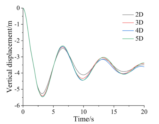
Fig. 18. Vertical displacement curve. |
Table 6. The draught value at different fluid field dimensions. |
| Fluid field dimension/D | Simulated draught value/m | Theoretical draught value/m |
|---|---|---|
| 2 | 3.521 | 3.446 |
| 3 | 3.567 | |
| 4 | 3.643 | |
| 5 | 3.583 |
4. Modeling method of vibration analysis considering ship-ice-water-air full coupling
In the ship-water‒air coupled vibration analysis, the ice load is applied to the hull structure for calculation, and the calculation scale mainly depends on the mesh sizes of the three. The role of water and air is also to ensure the correct floating state in the ship-ice-water coupled vibration analysis, which can follow the element size of water and air and mainly determine the model range. The role of the ship is to predict the structural vibration response, which is mainly to determine the element size of the excitation source near and the location of the vibration measurement points, and the division schematic is shown in Fig. 19.

Fig. 19. Schematic diagram of the meshing of the ship-water‒air coupling vibration model. |
4.1. Modeling method of ship structure
When using the FEM/BEM method for the prediction of structural vibration and noise in ships, the number of meshes increases with increasing frequency. For large vessels, the scale of the computational model is often unacceptable, and structural vibrations transmit energy in the hull mainly in the form of bending waves. In the region close to the vibration source, the structural vibration is larger and the vibration velocity declines faster, while the structural mesh scale is smaller in this region. In the region farther away from the vibration source, the structural vibration is smaller and declines slower, while the mesh scale is larger. Therefore, a gradient meshing model can be used for vibration and noise prediction of large-scale ship structures, the core of which is to determine the meshing size and division range [37].
According to fluctuation theory, the vibration wave mainly transmits energy in the form of a bending wave in the hull structure, which is attenuated by the damping effect of the structure. Generally, there should be at least 6∼8 nodes in one wavelength:
$\Delta \leq \frac{\lambda}{6}$
The wavelength of the bending wave in the plate is:
$\lambda_{B}=\frac{C_{B}}{f}$
The wave speed of the bending wave is:
$C_{B}=0.535 \sqrt{2 \pi h C_{l} f}$
$C_{l}=\sqrt{\frac{E}{12 \rho\left(1-u^{2}\right)}}$
Bringing Eqs. (4) and (5) into Eq. (2) gives the maximum element size equation:
$\Delta \leq 0.0892 \sqrt{2 \pi h C_{l} / f}$
where h is the plate thickness; E is the material modulus of elasticity; u is the Poisson's ratio; ρ is the density; f is the frequency; Cl is the longitudinal wave speed in the plate; CB is the bending wave speed in the plate; and λB is the bending wavelength in the plate.
The hull structure is composed of a large number of plates and beams. According to fluctuation theory, the propagation formula of a bending wave in an infinite beam structure is as follows:
$y(x)=y(0) e^{-j k x} e^{-\frac{1}{2} \zeta k|x|}$
where y(0) is the amplitude at the point of excitation; x are the coordinates with the excitation point as the origin and the beam length direction as the x-axis; k is the number of bending waves; and ζ is the damping ratio of the structure.
The wave velocity and the number of bending waves in the beam are as follows:
$C_{T}=4 \sqrt{\omega^{2} \frac{E I}{\rho A}}$
$k=\frac{2 \pi}{\lambda_{B}}=4 \sqrt{\frac{\rho A \omega^{2}}{E I}}$
where ω is the natural frequency; EI is the stiffness of the average straight beam; and A is the cross-sectional area of the beam.
Bring Eq. (9) into Eq. (7) gives:
$y(x)=y(0) e^{-j 4 \sqrt{\frac{\rho A \omega^{2}}{E l}} x} e^{-\frac{1}{2} \zeta 4 \sqrt{\frac{\rho A \omega^{2}}{E I}}|x|}$
For regions where the vibration response is less than $\frac{y(0)}{N}$:
$\frac{y(x)}{y(0)}=e^{-j 4 \sqrt{\frac{\rho A \omega^{2}}{E T}} x} e^{-\frac{1}{2} \zeta 4 \sqrt{\frac{\rho A \omega^{2}}{E I}}|x|}=\frac{1}{N}$
Neglecting the phases, the minimum length of the refined model region of the beam structure is obtained as:
$x=\frac{2 \ln (N)}{\zeta 4 \sqrt{\frac{\rho A \omega^{2}}{E T}}}$
Similarly, the minimum length of the refined model region for the plate structure is:
$x=\frac{2 \ln (N)}{\zeta} 4 \sqrt{\frac{E h^{2}}{12 \rho\left(1-u^{2}\right) \omega^{2}}}$
Based on fluctuation theory, it is known that the division range can be determined by Eqs. (12) and 13, and Eq. (6) can determine the maximum meshing size. Thus, the mesh division criterion for the gradient meshing model is realized. For the numerical analysis of ship-ice collision-induced vibration, the third gradient mesh is used to determine the division range for the regional structure close to the vibration source by Eq. (13), and the maximum meshing size for mesh division is determined by Eq. (6). The second gradient mesh is used for the superstructure and other areas far from the source, and the mesh size is uniformly divided using the frame space. The first gradient mesh is used to divide the mesh size of the structure using the strong frame size for the midship area.
In addition to the influence of high-power devices such as engines and propellers, the hull vibration of polar navigation ships also has ice-induced vibration caused by the ice-breaking load. The vibration sources are located in the bow and stern areas of the ship and are numerous. Therefore, a third gradient mesh is used for the area below the waterline at the bow and stern, a second gradient mesh for the area above the waterline at the bow and stern, and a first gradient mesh for the midbody area. The schematic diagram of gradient meshing is shown in Fig. 20.
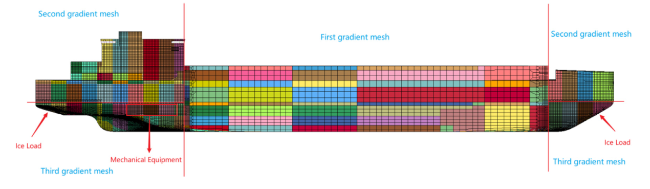
Fig. 20. Schematic diagram of gradient meshing. |
The density of the hull structure is known to be 7850 kg/m3, the modulus of elasticity is 2.01×10¹¹ Pa, and the Poisson's ratio is 0.3. The thickness of the plate is 36.5 mm in the ice-breaking area of the bow, and the thickness of the plate is 32.5 mm in the ice-breaking area of the stern. The frequency of the ice-breaking load is mainly within 100 Hz. The size of the third gradient mesh of the polar icebreaker is calculated according to Eq. (6). The size of the third gradient mesh is 169 mm in the collision region of the bow, and the size of the third gradient mesh is 160 mm in the collision region of the stern. When there is steady-state excitation, the third gradient mesh of the stern can be applied to the prediction of the vibration response of the stern by simply refining the meshing again at the main engine foundation. When there is transient excitation, the third gradient mesh of the bow and stern can be applied to the prediction of the ice-breaking vibration response. This also meets the meshing size requirements for ship-ice collisions. The mesh size requirements can be guaranteed, which include steady vibration, transient vibration, and ship-ice collision calculations, and the vibration response will provide a more accurate prediction during ice breaking.
4.2. Modeling method of level ice
Since the calculation method of complete ship-ice collision-induced vibration is too difficult, this paper applies the ice load of the ship-ice-water‒air coupled collision calculation as transient excitation on the hull structure to obtain the vibration response at different positions. However, the ice load involves two variation factors of time and area, and the effect on the results is larger when applied directly to the hull structure. Therefore, the area and loading method of the ice load need to be considered to apply the ice load more reasonably. First, the maximum value on the time domain curve of the collision force is selected, and then the loading area and the average pressure of ice load are determined according to the Requirements Concerning Polar Class of IACS Unified Requirements UR-II (IACS regulation). Finally, the location of the loading area is determined at the collision region of the elastoplastic ship model, and the average pressure is applied in this area to calculate the vibration response of the hull structure. The specific process is shown in Fig. 21 [38].

Fig. 21. Process of ice load transformation. |
To reflect the ice load of polar navigation ships of different ice classes in different areas, the IACS regulation divides the hull into four regions: Bow, Bow Intermediate, Midbody, and Stern. The calculation formulas of the ice load area and average pressure are selected according to the location of the ship-ice collision, as shown in Fig. 22. The collision location between a polar icebreaker and level ice is mainly the bow and stern, where the bow ice-breaking relies entirely on structural strength and mass, while the stern ice-breaking mainly relies on the propeller to break up large pieces of ice, and then the broken ice blocks collide with the hull structure. Taking bow ice-breaking as an example, the calculation formula of the ice load area and average pressure is determined according to IACS regulation [38].
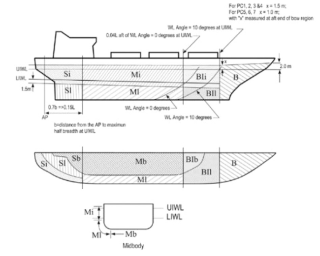
Fig. 22. Hull area extents. |
The ice load Fi, line load Qi, and pressure Pi of the bow area are determined as follows:
$F_{i}=f_{a i} \times \mathrm{CF}_{\mathrm{C}} \times \mathrm{D}^{0.64}[\mathrm{MN}]$
$\mathrm{Q}_{i}=F_{i}^{0.61} \cdot \mathrm{CF}_{\mathrm{D}} / \mathrm{AR}_{\mathrm{i}}^{0.35}[\mathrm{MN} / \mathrm{m}]$
$P_{i}=F_{i}^{0.22} \cdot \mathrm{CF}_{\mathrm{D}}^{2} \cdot \mathrm{AR}_{\mathrm{i}}^{0.3}[\mathrm{MPa}]$
where fai is the shape coefficient; CFC is the crushing failure class factor; D is the ship displacement [kt], which is not less than 5 kt; CFD is the load patch dimension class factor; and ARi is the load patch aspect ratio.
According to Eqs. (14)-(16), the load area of the bow area can be found as:
$\begin{array}{l} w_{\text {Bow }}=\frac{F_{\text {Bow }}}{Q_{\text {Bow }}}[\mathrm{m}] \\ b_{\text {Bow }}=\frac{Q_{\text {Bow }}}{P_{\text {Bow }}}[\mathrm{m}]\end{array}$
where FBow is the maximum force Fi in the Bow area [MN]; QBow is the maximum line load Qi in the Bow area [MN/m]; PBow is the maximum pressure Pi in the Bow area [MPa]; and wBow and bBow are the width and height of the design load patch, respectively.
The average pressure, Pavg, within a design load patch is determined as follows:
$P_{\text {avg }}=\frac{F}{b \times w}[\mathrm{MPa}]$
where F=FBow; b=bBow; w=wBow.
4.3. Modeling method of air and water
For the model range of the fluid field in vibration analysis, it is usually advisable to take more than twice the maximum bending wavelength of the analyzed frequency or directly take five times the ship width. Li [39] verified that the computational results converge when the fluid field model size exceeds four times the ship's width. To guarantee both computational accuracy and efficiency, it is suggested that the model range of the fluid field should be five times the ship width. The model range of the fluid field is also above 5 times the ship width in the ship-ice-water‒air coupled collision calculation. Therefore, combining the two conclusions to determine the width of the fluid field model in the ship-water‒air coupled vibration analysis can be consistent with the width in the ship-ice-water‒air coupled collision analysis, and the length can be twice the ship length and above. The calculation model of ship-water‒air coupling vibration is shown in Fig. 23.

Fig. 23. Calculation model of ship-water‒air coupling vibration. |
5. High efficient S-ALE coupling algorithm for dynamic problems
5.1. Principles of the S-ALE algorithm
The Arbitrary-Lagrangian-Eulerian (ALE) algorithm mainly solves the fluid-structure interaction (FSI) problem by considering the fluid's influence in LS_DYNA. The equations of conservation control of mass, momentum, and energy are given by introducing relative velocity w (w=v−u, where v is the speed of matter and u is the speed of the element), and then the master and slave contact surfaces are set by the penalty function method to realize the coupling of fluid-structure interaction. When a penetration occurs, a series of ordinary springs are automatically set between the master and slave contact surfaces to limit the occurrence of penetration by spring force [40].
$\frac{\partial \rho}{\partial t}=-\rho \frac{\partial v_{i}}{\partial x_{i}}-w_{i} \frac{\partial \rho}{\partial x_{i}}$
$v \frac{\partial v_{i}}{\partial t}=\sigma_{\mathrm{ij}, \mathrm{j}}+\rho b_{i}-\rho w_{i} \frac{\partial v_{i}}{\partial x_{j}}$
$\rho \frac{\partial E}{\partial t}=\sigma_{\mathrm{ij}} v_{i, j}+\rho b_{i} v_{i}-\rho w_{j} \frac{\partial E}{\partial x_{j}}$
where ρ is density; bi is force; E is energy; σij is the stress tensor; τ is shear stress; and P is pressure.
The ALE algorithm has the characteristics of geometry and element overlap of structure and fluid, which can reduce the calculation time of fluid-structure coupling problems. However, it is still difficult to calculate the large-scale fluid-structure coupling. To improve the efficiency and time of large fluid-structure coupling calculations, LS_DYNA adds a new Structured-ALE (S-ALE) algorithm based on ALE algorithm theory. The difference between the two algorithms is mainly the simplification of the operation of the structured element modeling. The ALE algorithm mainly relies on user definitions, which need to be generated in advance in the preprocessor and then read one by one. The S-ALE algorithm directly inputs the geometric size and spacing information in the calculation file, avoiding reading the nodes of all the elements used by the structured element one by one. Meanwhile, the subsequent modification of the element size is simplified, completely changing the idea and scale of modeling, as shown in Figs. 24 and 25. Therefore, the S-ALE algorithm has a reliable price reduction modeling method compared with the traditional ALE algorithm, which allows it to run faster with less memory and more stable computations. These advantages give the S-ALE algorithm broader application prospects in calculating large-scale fluid-structure interaction problems [40].
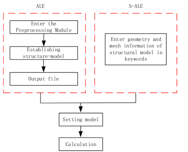
Fig. 24. Diagram of modeling process comparison. |
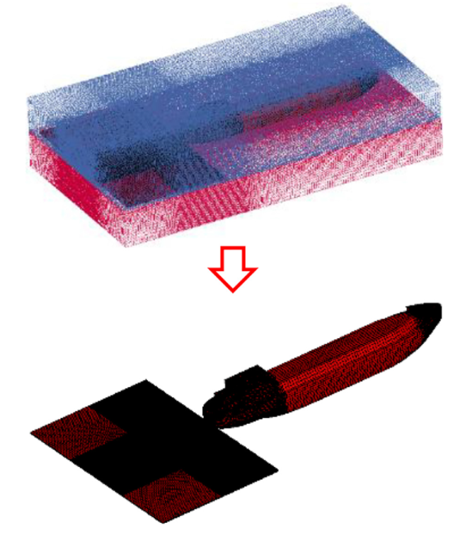
Fig. 25. Diagram of modeling transition. |
5.2. Comparison of the computational efficiency of ALE and S-ALE algorithms
To obtain a clearer understanding of the difference in computational efficiency between the two algorithms, the computational model of ship-ice-water‒air coupling collision in Fig. 26 was used to analyze the variation in memory usage and actual time taken by the two algorithms for the same number of elements, nodes, computation time, and cores. The total computer resources used included 256 GB of memory, 2.50 Hz main frequency, 28 cores, and a Win10 system.

Fig. 26. Model of ship-ice-water‒air coupling collision. |
It can be seen in Table 7 that the S-ALE algorithm reduces the memory by 35.23% and the actual time consumption by 47.86% compared with the traditional ALE algorithm. Therefore, the S-ALE algorithm is suitable for large-scale ship-ice-water‒air coupling calculations.
Table 7. Comparison data of computing resources. |
| Method | Number of elements | Number of nodes | Computation time | Cores | memory | actual time |
|---|---|---|---|---|---|---|
| ALE | 609,120 | 715,299 | 10s | 16 | 30.249944MB | 158 h38 min |
| S-ALE | 19.592610MB | 82 h43 min | ||||
| Comparison | - | - | - | - | 35.23% | 47.86% |
6. Conclusion
This paper systematically investigates methods that can be used for the numerical analysis of ship-ice collision-induced vibration. First, ideal and simplified analysis methods are studied for the ship-ice collision-induced vibration problem, and the advantages and processes of the four-phase ship-ice-water‒air coupling method are analyzed. Second, the mesh sizes and model ranges of the ship, level ice, water, and air models are determined based on the simplified numerical analysis of the ship-ice collision-induced vibration, and the conversion method of ice load is given in the vibration analysis of a fully coupled ship-water‒air problem. Finally, the highly efficient S-ALE algorithm is introduced based on the ALE algorithm, and the computational efficiency of the ALE and S-ALE algorithms are compared.
(1) For the numerical analysis of ship-ice collision-induced vibration, a simplified numerical analysis method can be used to predict the vibration response of the ship structure during the ice-breaking process. This method considers the coupling effects of four media: ship, level ice, water, and air. It can simultaneously realize the effects of fluid resistance and the gravity field on the floating state of a surface object and improve the calculation accuracy.
(2) In the ship-ice-water‒air coupling collision problem, the element size of the ship is 250×250 mm, the element size of the level ice is 0.5 × 0.5 × 0.5 m, and the element size of the fluid field is 1 × 1 × 1 m. The modeling range of level ice is six times the ship width and one time the ship length for the ship model. The horizontal dimension of the water and air can be determined by the ship and sea ice scale. The vertical dimension of the air can be chosen between the draught and the depth of the ship, which is higher than the maximum height of the ship. The vertical dimension of the water can be chosen between one time the depth and above. The above element size and modeling range can be directly implemented in the numerical simulation analysis of the ship-ice-water‒air coupling collision problem below the current speed.
(3) In the ship-water-air coupling vibration problem, the bow and stern of the polar ice-breaking transport vessel are refined according to the principle of gradient meshing. The mesh size of the bow is 169 mm, and the stern is 160 mm. The width range of the fluid field model is consistent with the width range in the ship-ice-water‒air coupled collision analysis, and the length is adopted as two times the ship length and above. This model can achieve the calculation requirements of both steady-state vibration and ice-induced vibration, which provides a basis for the study of steady-state and transient coupled vibration response of polar ships.
(4) The full coupling method of ship-ice-water‒air can simulate the ship-ice collision-induced vibration analysis problem more reasonably and effectively, which is of great help to the actual ice load and vibration response prediction of the ship. Meanwhile, the S-ALE algorithm has obvious advantages for the problems of large-scale fluid-structure coupling and can improve computational efficiency.
Declaration of Competing Interest
The authors state that they have no competing financial interests or personal relationships that can influence the work reported in this paper.
CRediT authorship contribution statement
Yuan-He Shi: Conceptualization, Writing - original draft, Writing - review & editing, Formal analysis, Validation. De-Qing Yang: Methodology, Supervision, Writing - review & editing, Project administration. Wen-Wei Wu: Methodology, Conceptualization.
Acknowledgment
The study is supported by the National Ministry of Industry and Information Technology of China. The authors would like to acknowledge the project's support.
