
1. Introduction
There are many offshore activities developed rapidly in the past decades such as gas and oil exploration and storage, deep sea expedition, and military missions [1,2]. Offshore floating platforms and vessels usually move in six degrees of freedom (DoF) excited by environmental forces, such as wave, ocean current or wind. The motions would bring up remarkable challenges to carry out offshore works, which limits many motion-sensitive activities. The real-time motion predictions of a floating platform or a vessel usually refer to predicting the motions of vessel in a short period of time [3]. It is meaningful to predict the real-time motions, as the performance of a motion compensation system can be enhanced. Besides, it can also give us useful early-warning information that is significant with regard to motion. The landing of an aircraft on a carrier also requires real-time motion predictions to improve the performance.
The dynamic motion responses of offshore platforms were deeply explored. Although excitations of environmental forces in real sea states are random, it is believed that the dynamic process is ergodic and stationary [4]. In the traditional analysis, the motion responses are usually demonstrated by response spectra or response amplitude operators (RAOs) about concerning the frequency domain. Besides, in the time domain, the statistical values such as mean, standard deviation, and some significant values are described. Such analysis is usually performed in the time domain or frequency based on series data from 3-h experiments or simulations. The spectra and statistical values are applied as key features to illustrate the motions. These results make contributions to the safety design of offshore platforms. However, the exact motions of the offshore platform motion are not illustrated in a short period of time.
The Kalman filtering technique has been used by Triantafyllou and Athans [5⇓-7] to predict vessel motions up to 5 s. The Kalman filter requires the state-space vessel model which is based on the full knowledge of hydrodynamics. As the damping, added mass, and wave excitation forces depend on frequency, it is crucial to estimate the peak frequency of the wave spectrum. Recently, there were some developed systems for real-time prediction of vessel motions [8,9], which were based on vessel seakeeping and nonlinear wave theories. These models require full knowledge of hydrodynamics. Direct analysis of time series such as the auto-regressive (AR) models does not require the prior knowledge about the responses of ship. It was demonstrated by Yumori [10] that an auto-regressive moving average model could predict the ship behavior about 2 to 4 s ahead.
Nowadays, machine learning [11⇓-13] is a popular field as it can provide us with a powerful framework to learn the features directly from the data without much knowledge about underlying physics. The trainable parameters in the machine learning model are determined by minimizing the loss between its predictions and ground truths. Sclavounos and Ma [14] applied the support vector machines to forecast a short-term wave in 5 s with good accuracy. Khan et al. [3] obtained the roll motion predictions up to 7 s by applying a three-layer fully connected neural network model. Li et al. [15] employed the artificial neural network to forecast the wave-excitation force in 2.5 s for a controller of the wave energy converter.
The well-known recurrent neural networks (RNNs) [16,17] have been successfully used in sequential data processing such as time series, speech, and language. The RNNs encode the temporal dependence of inputs into the history of the system dynamics. The long short-term memory (LSTM) model [18] is a type of RNN, which has been used to predict the heave and surge motions of a semi-submersible from a model test about one wave cycle if only based on the motion data [19].Especially, it is worth noting that a machine learning technique known as reservoir computing (RC) has good performance in forecasting some complex dynamical systems [20⇓⇓⇓⇓⇓⇓-27]. The framework of RC is derived from the RNN and is thus suitable for sequential/temporal information processing. The low-dimensional input vector is fed into a high-dimensional phase space called a reservoir. The internal network weights in the reservoir are specified by the adjacency matrix. The matrix is a sparse directed random matrix, whose elements are predetermined and not trained. And the readout weights for pattern analysis are trained to map the reservoir state to the desired output. Therefore, the RC model can alleviate the difficulty to learn the recurrent connections of standard RNNs and decrease the training cost.
In this paper, we propose the strategy to make the predictions of heave, surge, and pitch motions of a moored rectangular barge based on the RC model. The 3-DoF motions are excited by an irregular wave. The machine learning model is obtained only based on the 3-DoF motion data. The dataset came from a model test carried out in the deep-water ocean basin, at Shanghai Jiao Tong University, China. After training, the machine learning model can provide the predictions of surge, heave, and pitch motions for about two to four wave cycles with good accuracy. Thus, the machine learning model shows great potential to predict the motions of offshore vessels or platforms.
The rest of the paper is organized as follows. In Section 2, we describe the model test of moored rectangular barge which generated a dataset for the machine learning. In Section 3, we describe the basic idea of the machine learning technique - reservoir computing. In Section 4, we illustrate the training process and performance of the machine learning model. Finally, Section 5 presents the concluding remarks.
2. Model test
In this section, we illustrate a scaled model test carried out in the deep-water wave basin at Shanghai Jiao Tong University (SJTU), China, which generated a dataset for the machine learning model.
The length and width of wave basin are 50.0 m and 40.0 m, respectively. The wave basin is up to 10 m in depth with a large-area movable bottom. The wave maker was equipped to model ocean waves in the basin. The passive wave absorbing beach was equipped with damping grids and an optimized parabola profile for wave dissipation. The scaled model of rectangular barge is shown in Fig. 1(a). Fig. 1(b) presents the in-place model during testing. The scaled ratio was set to 1: 64. The main dimensions and properties of this rectangular barge are listed in Table 1. As shown in Fig. 2, the model was moored in the deep wave basin by 4 horizontal mooring lines attached to the model at the corners. The horizontal mooring system provided restoring force. An optical motion capture system was used for capturing the six-DoF motions. The irregular wave was generated following the JONSWAP spectrum as follows,
$ S(f)=\alpha H_{s}^{2} T_{p}^{-4} f^{-5} \exp \left[-1.25\left(T_{p} f\right)^{-4}\right] \gamma^{\exp \left[-\frac{\left(T_{p} f-1\right)^{2}}{2 \sigma^{2}}\right]},$
where γ=2 is the shape parameter, Tp is the spectral peak period, Fp=1/Tp is the spectral peak frequency, σ = 0.09 for f>Fp and σ=0.07 for f<Fp, and Hs is the significant wave height. The specified wave elevations were calibrated before starting the model test. The significant wave height Hs is 9.9 m and the spectral peak period Tp is 11.9 s in the prototype.

Fig. 1. Pictures of (a) the rectangular barge model and (b) the model tested in water. |
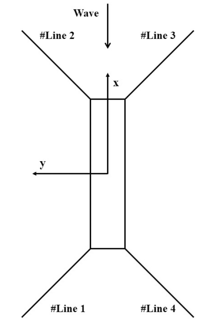
Fig. 2. Top view of the moored rectangular barge in the wave basin. |
Table 1. The main dimensions and properties of the rectangular barge. |
| Parameter | Unit | Prototype | Model |
|---|---|---|---|
| Hull length | m | 213.312 | 3.333 |
| Hull width | m | 49.088 | 0.767 |
| Normal Draft | m | 11.84 | 0.185 |
| Nominal Displacement | t | 123520.29 | 0.4597 |
| Vertical center of gravity | m | 17.344 | 0.271 |
| Longitudinal Center of Gravity | m | 106.688 | 1.667 |
| Roll gyradius | m | 15.808 | 0.247 |
| Pitch gyradius | m | 67.84 | 1.06 |
Instead of the barge model, three wave probes were placed at the center of the basin to record the wave elevation for wave calibration. Fig. 3(a) presents the time series of the wave elevation at the center of basin and Fig. 3(b) shows the corresponding power spectrum density compared with theoretical results. After the calibration of wave, the model was put into the basin and moored by the horizontal mooring system. Then, the waves were generated and motions are synchronously recorded for longer than 30 min (corresponding to 3 h in the prototype). The sampling rate was set at 25 Hz in the model scale corresponding to 3.125 Hz in the prototype. The head wave mainly excited the surge, heave and pitch motions of the barge. Therefore, we consider these 3-DoF motions in this study.
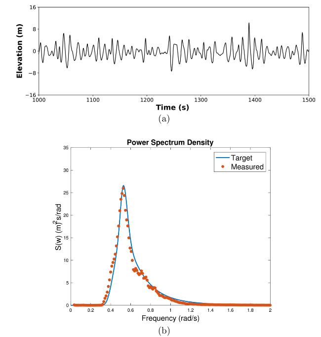
Fig. 3. The time history of the wave calibration (a) and the power spectrum density of the wave calibration compared with the target JONSWAP wave (b). |
Finally, the dataset generated from the model test for machine learning consists of 43,000 sampling points, i.e. 13,760 s. The statistics of surge, heave, pitch motions, and wave calibration in the prototype are shown in Table 2, including the maximum value, minimum value, mean, standard deviation, significant positive single amplitude, significant negative single amplitude, and significant double amplitude.
Table 2. Statistics of time domain of the 3-DoF motions of the rectangular barge and the wave calibration from the model test in the prototype. |
| Title | Unit | Max | Min | Mean | Std | Pos.Sign. | Neg.Sign. | Dou.Sign. |
|---|---|---|---|---|---|---|---|---|
| Surge | m | 12.68 | −18.34 | −1.86 | 3.81 | 7.00 | −7.34 | 13.81 |
| Heave | m | 1.93 | −2.52 | 0.04 | 0.61 | 1.20 | −1.23 | 2.36 |
| Pitch | deg | 4.67 | −4.81 | 0.01 | 1.44 | 2.82 | −2.87 | 5.61 |
| Wave | m | 14.82 | −10.28 | 0.00 | 2.44 | 5.69 | −4.54 | 9.78 |
3. Reservoir computing model
A machine learning technique known as “Reservoir Computing” (RC) model has been proven to be effective for the prediction of many complex dynamical systems [20⇓⇓⇓⇓⇓⇓-27]. The framework of RC is derived from the RNN and it can alleviate the difficulty to learn the recurrent connections of standard RNNs and decrease the training cost [27]. We demonstrate the main idea of the reservoir computing in this section.
An input vector u(t) of dimension Din is fed into a “reservoir” of dimension Dr through an I/R (input-to-reservoir coupler). An output vector v(t) of dimension Dout is coupled from the reservoir through an R/O (reservoir-to-output coupler). The general approach is illustrated in Fig. 4(a). The reservoir is a large, low-degree (κ) random network, with a Dr×Dr adjacency matrix A. The elements of A are chosen from a uniform distribution in [0,α], where α>0 is adjusted to make the largest eigenvalue of A (the spectral radius of A) equal to the desired value r. Following [21], [24], the functions of I/R and R/O can be represented in discrete time (t=0,Δt,2Δt,) with the specific implementation given by
$ \mathbf{r}(t+\Delta t)=\tanh \left[\mathbf{A r}(\mathrm{t})+\mathbf{W}_{\mathrm{in}} \mathbf{u}(\mathrm{t})\right]$
$ \mathbf{v}(t+\Delta t)=\mathbf{W}_{\text {out }}(\mathbf{r}(t+\Delta t), \mathbf{P})$
where r(t) represents the scalar states ri(t) (i = 1, 2,..., Dr) of the reservoir nodes; Win is a Dr×Din matrix, which maps the input u(t) to the reservoir state r(t); Wout is a Dout×Dr matrix, which maps r(t) to the output v(t). The elements of Win are chosen from a uniform distribution in [−σ,σ] and every node in the reservoir receives one scalar input from u(t), where each scalar input is connected to Dr/Din nodes in the reservoir. Wout depends on adjustable parameters given by the elements of the matrix P. Here, we define Wout as $ \mathbf{W}_{\text {out }}(\mathbf{r})=\mathbf{P}_{1} \mathbf{r}+\mathbf{P}_{2} \mathbf{r}^{2}$, where $ \mathbf{P}=\left(\mathbf{P}_{1}, \mathbf{P}_{2}\right)$ and the matrix elements in even columns of P1 and odd columns of P2 are set to be zeros. The goal of the system is to make v(t) approximate the target outputs vd(t). To accomplish this, during a training period −T⩽t⩽0, the input u(t) is fed into the reservoir, and the resulting r(t) along with u(t) are prerecorded. The output parameters P are chosen in order to minimize the least difference between v(t) and vd(t). The Tikhonov regularized regression procedure [28] is used to obtain an output matrix P, that minimizes the following function
$ \sum_{-T \leqslant t \leqslant 0}\left\|\mathbf{W}_{\text {out }}(\mathbf{r}(t), \mathbf{P})-\mathbf{v}_{d}(t)\right\|^{2}+\beta\|\mathbf{P}\|^{2}$
where β>0 is used to discourage over-fitting by penalizing large output weights.
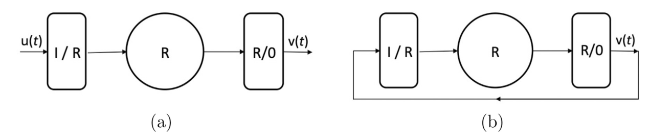
Fig. 4. The architecture of machine learning technique - reservoir computing model. (a) Training phase; (b) Predicting phase. |
$ \mathbf{r}(t+\Delta t)=\tanh \left[\operatorname{Ar}(\mathrm{t})+\mathbf{W}_{\text {in }} \mathbf{W}_{\text {out }}(\mathbf{r}(\mathrm{t}))\right]$
The predictions are then given by $ \mathbf{v}(t)=\mathbf{W}_{\text {out }}(\mathbf{r}(t))$. If one wants to predict the u(t) for t>t0 based on the true measurements of u up to time t0. The reservoir model can be reinitialized using Eq. (5) for a short period of time τ before t0 i.e., (t0−τ≤t≤t0), to determine the r(t0), and then can be used to predict time series for t>t0.
4. Machine learning prediction
In this section, we illustrate the strategy of using the machine learning technique - reservoir computing model to predict the 3-DoF (surge, heave, and pitch) motions of the moored rectangular barge, purely based on the motions data. Then, the predictions given by the machine learning model are evaluated.
We use the records from the model test in the prototype with 43,000 sample points (corresponding to 13,760 s) as the dataset. The timestep of sample points is 0.32 s. The first 38,000 samples (t∈[0,12160]s) of 3-DoF motion data are used as the training data to train the reservoir computing model. The next 1000 samples (t∈[12,160,12,480]s) are used as the validation set to determine the hyper-parameters of the reservoir computing model. And the last 4000 samples (t∈[12,480,13,760]s) of motion data are used as the test set to evaluate the generalization capability of the trained machine learning model.
First, we do the data prepossessing of motions before we put the data into the reservoir computing model. The 3-DoF motion data have different characteristics as the surge and heave are measured in meters while the pitch is measured in degrees. Besides, the magnitudes of the 3-DoF motions are also different. Thus, the data are normalized to eliminate the influence of dimensions, and maintain the stability and accuracy of the training process. Each motion data is normalized as follows,
$ \tilde{x}_{i}(t)=\frac{x\left(t_{i}\right)-a}{b} \text {, }$
where a and b are the mean and standard of the training dataset. Finally, we scale up the outputs to obtain the actual results.
The grid search is performed for determining the hyper-parameters (r,σ,β,κ) of the reservoir model by evaluating the predictions in 20 different initial conditions in the validation set with 200 time steps, i.e. 64 s. The hyper-parameters are chosen as the reservoir model prediction has the smallest mean absolute error in the validation set. In the prediction phase, as illustrated in Section 3, actual motion data with τ=50 time steps (i.e. 16 s) before the prediction start time are used to warm up the reservoir states. It is found that the larger value of τ would not improve the performance of reservoir predictions and thus the 50 time steps of true measurements are enough. Finally, the hyper-parameters of the reservoir computing model are chosen as shown in Table 3. Once the reservoir computing model is trained and the weights of the model are determined, the model can then be used to make a series of predictions for 3-DoF motions from any given start time.
Table 3. Hyper-parameters of the reservoir model for predicting the 3-DoF motions. |
| Hyper-parameter | r | σ | β | Dr | τ | κ |
|---|---|---|---|---|---|---|
| Value | 0.9 | 0.1 | 1e−7 | 3000 | 50 | 3 |
Then, we evaluate the performance of this machine learning model by using the trained reservoir computing model to make the predictions of surge, heave and pitch motions in the test set with t∈[12,480,13,760]s. We make the predictions of 3-DoF motions of the moored rectangular barge from 70 different initial conditions in the test set, which start from different values of t0 as t0=(12,480+16×k) s, where k is an integer ranging from 0 to 69. Fig. 5, Fig. 6, Fig. 7 present some examples of machine learning predictions of surge, heave, and pitch motions respectively in the test set, Fig. 8(a)-(c) show the overall mean absolute errors (MAEs) over the 70 predictions in the test set with different prediction lengths. The overall MAEs of the predictions in the test set are about 1.01 m for the surge predictions in 50 s, 0.23 m for heave predictions in 20 s, and 0.42 m for the pitch predictions in 30 s. The relative values of MAEs compared with the corresponding significant double amplitude of motions in Table 2 are about 0.073, 0.097 and 0.075 for surge, heave and pitch, respectively. It is illustrated that the machine learning model can predict the surge, heave and pitch motions for about 50 s, 20 s, and 30 s with good accuracy, respectively.
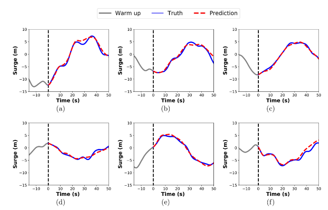
Fig. 5. Examples of surge motion predictions given by the machine learning model in the test set. Grey line: the true measured data used to warm up the state of machine learning model; Blue line: the true measured data; Red dashed line: the machine learning predictions. |
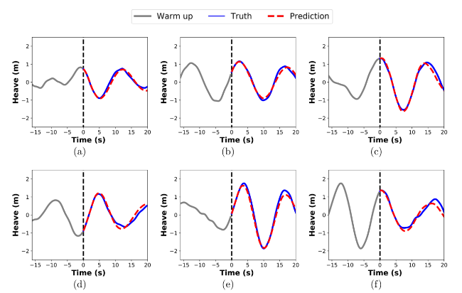
Fig. 6. Examples of heave motion predictions given by the machine learning model in the test set. Grey line: the true measured data used to warm up the state of machine learning model; Blue line: the true measured data; Red dashed line: the machine learning predictions. |
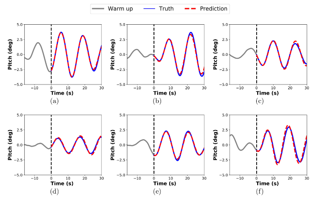
Fig. 7. Examples of pitch motion predictions given by the machine learning model in the test set. Grey line: the true measured data used to warm up the state of machine learning model; Blue line: the true measured data; Red dashed line: the machine learning predictions. |
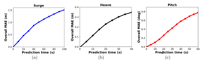
Fig. 8. The overall mean absolute errors (MAEs) of machine learning predictions in the test set with different prediction lengths for (a) surge, (b) heave, and (c) pitch. |
Therefore, using this data-driven machine learning model based on the 3-DoF motions of the moored rectangular barge, we are able to make predictions of surge, heave, and pitch motions up to several wave cycles into the future. It is meaningful to predict the real-time motions in practice, as the performance of a motion compensation system can be enhanced. Besides, it can also give us some useful early-warning information with regard to motions. The landing of an aircraft on a carrier also requires real-time motion predictions to improve the performance.
5. Concluding remarks
Many offshore activities and naval exploration are motion-sensitive, such as oil and gas exploration and storage, and aircraft landing. Therefore, it is significant to predict the real-time motions of a floating platform or a vessel, which can enhance the performance of a motion compensation system and provide us with helpful early-warning information.
In this work, we propose the strategy to predict the surge, heave, and pitch motions of a moored rectangular barge based on the machine learning technique. The dataset came from a model test performed at SJTU deep-water ocean basin, China. The motions of the moored barge were excited by an irregular wave. The reservoir computing model is applied to make future predictions purely based on the 3-DoF motion data of the barge. The trained machine learning model can provide predictions of the surge, heave, and pitch motions for about two to four wave cycles with good accuracy. The machine learning model can provide us with a powerful framework to learn the features directly from the data without prior knowledge about underlying physics. It shows the great potential for applying the machine learning technique to predict the motions of off-shore platforms or vessels.
Declaration of Competing Interest
Authors declare that they have no conflict of interest.
Acknowledgments
This work is partly supported by Shanghai Pilot Program for Basic Research - Shanghai Jiao Tong University (No. 21TQ1400202).
