
Glossary
Acronyms
AI: artificial Intelligence
ANN: Artificial Neural Networks
BEM: boundary element method
GPU: graphics processing unit
MAE: mean absolute error
MLP: multi-layer perceptron
MNRE: mean normalized relative error
NRE: normalized relative error
Ship parameters
: cross-sectional area
: waterplane area
: midships cross-sectional area
: amidships longitudinal-sectional area
: waterline beam
: block coefficient
: amidships coefficient
: midships coefficient
: prismatic coefficient
: waterplane coefficient
: draught
: ship principal inertias
: waterline length
: longitudinal position of the buoyancy center
vertical position of the buoyancy center
: ship displacement
Fr: froude number
Wave parameters
k: wave number
T: wave period
: wavelength
: wave amplitude
: wave angular frequency
Seakeeping parameters
: dimensionless added mass matrix
: dimensionless damping matrix
: dimensionless wave excitation vector of forces
: dimensionless wave excitation vector of moments
Others
: gravity acceleration
: ANN predicted output
: target output
(*): dimensionless
1. Introduction. State of art
Thanks to the advantages offered by Artificial Intelligence (AI) and Machine Learning (ML) such as generalization ability, simplicity, adaptive learning, and others, ML are being used in many different fields of engineering. But not many ML techniques have been applied in marine engineering. Recently, Ao et al. [1] developed a Deep Learning algorithm capable to predict bare hull ship resistance. A database was generated using Free Form Deformation technique to get a large number of variations of the base containership KRISO. The targeted outputs were obtained using a potential flow code. Then they applied an optimization processes to the ANNs’ hyperparameters to obtain the best ANN. The resulting algorithm achieved promising results with an acceptable error when compared to the solver used to obtain the targeted output. Zhou et al. [2] optimized the hyperparameters using different ML techniques, such as, Artificial Neural Networks (ANNs), Support Vector Regression (SVR), and Random Forest (RF), in order to develop an algorithm capable of predicting fuel consumption taking into account weather and ship conditions. They concluded that ANNs algorithms can provide a robust and accurate estimation of fuel consumption.
Other as Cepowski [3,4] developed a set of ANNs capable of predicting added resistance in waves, sway accelerations, and roll angles for Car Carriers. The author used these ANNs to optimize car carrier ships. The main advantage of this set of ANNs is the ability to make predictions without needing the exact ship's hull geometry. They only require the length to beam (L/B) and beam to draft (B/T) ratios, and hull shape coefficients as inputs. However, these trained algorithms are only capable of make predictions for Car Carriers within a limited range of principal dimensions.
AI has also been applied to seakeeping computing. Sayli et al. [5] used Non-linear meta-models [6,7] to predict the heave and the pitch Response Amplitude Operators for fishing vessels in head waves. It was used 13 different hull shapes, combining V and U sections. And the draft was modified to obtain 39 different ships. Then, using strip theory, seakeeping loads were computed in order to get the target outputs for training the AI algorithm. They used traditional naval architecture coefficients as input for ANNs, as Cepowski in [3,4]. And similarly, to previous works, ML techniques were used but they were tailored for specific types of ship. Alarrcin et al. [8] developed an ANN algorithm for the control algorithm of a container ship dynamic roll stabilizer. They used supervised learning with the most used network in regression problems, the Multi-Layer Perceptron (MLP) [9,10], combined with backpropagation. This ANN model consists of one input layer, several hidden layers, and one output layer. The main achievement is an ANN algorithm for dynamic roll control capable of significantly reducing roll amplitudes.
Ekinci et al. [11] demonstrated that AI algorithms can be applied successfully to estimate ship design parameters such as the beam, waterline length, deadweight, and draft to improve the ship definition in the early stages of design. They analyzed different AI methods and applied ANNs to optimize a chemical tanker. Abramowski [12] analyzed the effective power and preliminary data of conventional cargo ships depending on the ship velocity, vertical position of center of gravity, displacement, and cost. This author combined ANNs with other techniques such as genetic and simulated annealing algorithms to optimize the ship design. ANNs algorithms were trained to include a wide range of ships. Abramowski concluded that the combination of those methodologies opens wide possibilities when compared to traditional approaches used in the early stages of the ship design.
Yu and Wang [13] investigated the minimization of the ship wave resistance in calm waters using the Multi-Layer Perceptron (MLP). The original database used to train the MLP was formed by four well know hull forms: S60 with block coefficient Cb = 0.6 and Cb = 0.7); S175 series; and Wigley hulls. They applied transformation techniques on those four parent ships to increase the database to thousand different geometries. The algorithms inputs were parameters obtained from a principal component analysis, and the target bare hull resistance was obtained by computational analysis.
More recently Taghva et al. [14] predicted heave, roll, and pitch RAOs and added wave resistance of container ship based on the S175 hull using ANNs. As previous works, traditional naval architecture parameters were used to train the ANNs. The strip theory method was used to compute the seakeeping and added resistance in wave results for training the ANNs.
Other uses of AI are aiming at basic conceptual ship design. Gurgen et al. [15] trained ANN algorithms to predict principal dimensions for the conceptual design of chemical tankers. In this case, the database consists of 100 tanker ships. And ANNs were trained with basic ships parameters, such as freeboard, deadweight, length overall, and others. After training the ANNs, they obtained high correlation coefficients, and showing that AI can be used to determine initial ship's particulars with high accuracy levels when compared to common regression methods.
ANNs can be sensitive to patterns between the input and the targets, difficult to reproduce with simple regression methods. However, the main drawback of ANNs is that they required large databases. For limited databases their advantages vanish and the risk of overfitting [9] increases, impeding generalization
Recently Águila et al. [16] trained Recurrent Neural Networks (RNN) to predict seakeeping of the DTMB combatant ship in the time-domain. They compared Gated Recurrent Units (GRUs) and Long Short-Term Memory (LSTM) and concluded that LSTM are the best option for this specific analysis. GRUs and LSTM are types of RNN that address the ability of memory from previous points in time to help the network for future predictions. In this work, the authors used an original approach in which continuous functionals were approximated by LSTM.
Cepowski [17] continued previous works [3,4], and trained ANNS to predict added wave resistance using basic ship design parameters such as the length, beam, draft, Froude number and wavelength. The author showed the ability of AI to predict complex quantities with few basic data. While only few types of ships (passenger and ferry ships) can be predicted in previous works [3,4], in [17] Cepowski extended his algorithms to a few more typologies of ships. The dataset to train ANNs consists of computational results from 14 types of ships. Added resistance in waves coefficients were predicted by MLP, and compared with experimental results achieving a high accuracy.
Based on this literature review, several conclusions can be made:
· There are vast experimental seakeeping results, but they are scattered, limited, and non-homogenized to use in massive AI training. Then the large datasets of results required for training AI algorithms are obtained by numerical computations.
· Previous works have shown that, for many marine engineering applications, traditional form coefficient and principal dimensions are enough to define the hull geometry and feed ANNs.
· In previous works, the authors usually focused on obtaining ANN algorithms for very specific types of ships with a very limited training database. This results in algorithms that cannot be used for a wide range of ships, and might lead to overfitting.
2. Aim of this work
The main objective of this work is the development of Artificial Neural Networks (ANNs) capable of predicting the seakeeping of conventional ships. We define a conventional ship as a monohull vessel operating in displacement conditions. These ANNs will predict the Froude Krylov and wave diffraction and radiation loads as those computed using a standard frequency-domain first-order wave diffraction-radiation solver based on the Boundary Element Method (BEM) [18,19]. These loads correspond to the incident wave load, added mass, damping, and wave diffraction loads, and hereafter will be refereed as seakeeping loads.
The purpose is to obtain a seakeeping tool capable of providing results instantly with an accuracy similar to those provided by a frequency domain BEM code. This tool will predict seakeeping based on basic hull form coefficients allowing to include seakeeping performance within the early stages of ship design.
This work is presented as follows: first it is introduced the methodology that has been used to model the seakeeping problem; second it is explained how the ANN training dataset has been obtain; third it is described how the different ANN architectures are generated, detailing the analyses carried out to select the best ANNs; fourth the results obtained from the ANNs are compared to those obtained by BEM for a number of ship shapes; and fifth results are discussed and conclusions are provided.
3. Methodology
The methodology used to generate the AI architecture is based on seven steps (see Fig. 1). These steps are as follows:
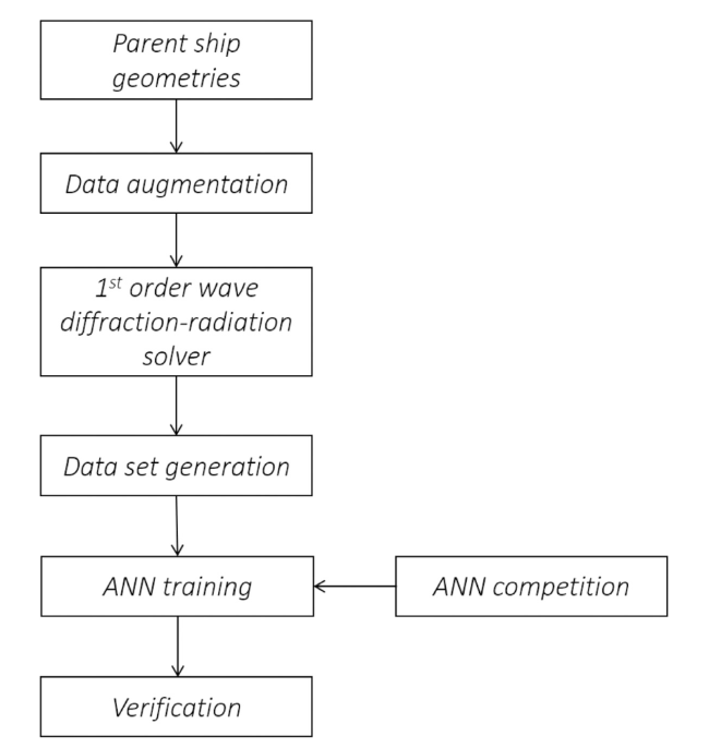
Fig. 1. Methodology employed to generate the ANN architecture. |
Step 1: Parent ships geometries database: Gathering of a parent ships database as broad as possible, including different types of conventional monohull ships (bulk-carriers, containerships, fishing vessels, etc.).
Step 2: Ships database augmentation [18]: The database is augmented by parametric variations of the beam-length and draft-beam ratios.
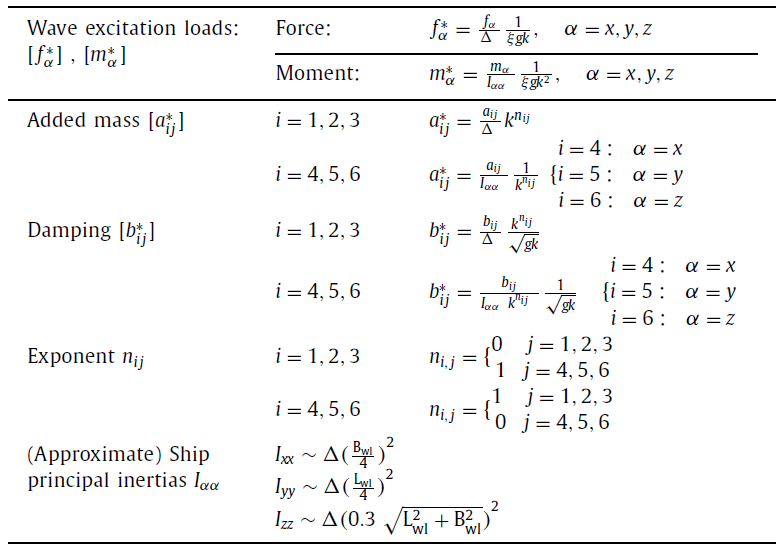
To carry out the comparison of results with a proper order of magnitude seakeeping loads are set dimensionless. Table 1 provides the corresponding dimensionless formulation for each hydrodynamics coefficient, taking as a reference term the diagonal term of the ship's mass matrix (displacement and approximate inertias using the shown expressions in Table 4). Then the dataset of results to train the ANNs is generated.
Table 1. Dimensionless seakeeping loads. |
 |
Step 5: ANN training: The ANNs are trained using the hull form coefficients as the input dataset. The targeted outputs Dataset is composed of: added mass and damping matrices, and excitation loads.
Step 6: ANNs competition: A competitive process among the different ANN architectures is carried out to select the best one (the one minimizing the errors).
Step 7: Verification: Finally, a verification process is carried out comparing the ANN results against BEM results for a number of ships not included in the parent ships database, and not used neither for the training nor for the validation.
4. Data mining and simulation
4.1. Generating the dataset
A dataset of seakeeping results for a large database of ships is required for training the ANN algorithms [20]. In this work, the database of ships is generated out of 50 different parent ship geometries, considering a wide range of ship types. Fig. 2 show the dimensionless cross-sectional area curves, and Tables 2 and A1 provide the form coefficients and the parent ships type.
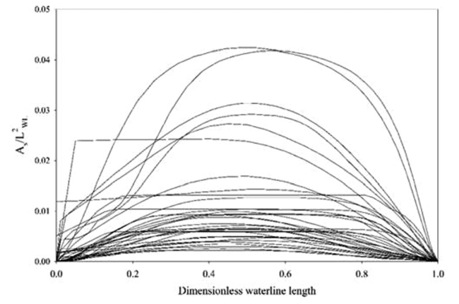
Fig. 2. Dimensionless cross-sectional area for each parent geometry. |
Table 2. Range of the dimensionless form coefficients for the parent ships. |
| Form coefficients | Range |
|---|---|
| Block coefficient Cb | 0.331-0.891 |
| waterplane coefficient Cwl | 0.625-0.946 |
| Midship coefficient Cm | 0.475-0.995 |
| Prismatic coefficient Cp | 0.522-0.901 |
| XB/Lwl | 0.391-0.554 |
| ZB/Lwl | −0.485-−0.276 |
For each parent ship, 400 hulls are generated using 20 parametric variations of length-to-beam and beam-to-draft ratios. The ranges for these ratios are $ 1.5 \leq \frac{\mathrm{L}_{\mathrm{wl}}}{\mathrm{B}_{\mathrm{wl}}} \leq 8.0< $ and $ 1.0 \leq \frac{B_{\mathrm{Bl}}}{\mathrm{D}} \leq 5.5 $. Then, the database of ships is based on 20,000 different hulls. Fig. 3 provides a spatial visualization for the database of ships used in this research. Fig. 4 shows the original geometry and two extreme parametric variations for a specific geometry. The output datasets are computed using the BEM for the 20,000 hulls.
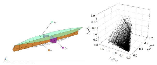
Fig. 3. Left: Amidship (Ac), midship (Am), and waterplane (Awl) sections of a ship. Right: Dataset representation based on sectional area ratios. |
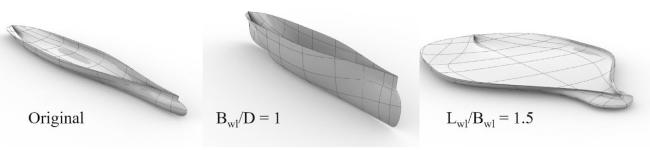
Fig. 4. Extreme parametric variation of a ship geometry. |
4.2. Seakeeping simulation particulars
In this work, a seakeeping BEM code, based on an improved version of Nemoh [18,22], is used to solve the first-order wave diffraction-radiation problem. A BEM code has been chosen instead of a strip code for several reasons. Based on Neumann [23] most strip theories are not valid for low frequencies. The strip theory does not have three-dimensional effects representing interactions between sections nor any forward-speed effects on the free-surface condition [24], compared with BEM formulation. Some comparison and validation about BEM code used can be found in a literature review. For instance, Parisella [25] compared the results of Nemoh with those computed by WAMIT [26], obtaining a low error. Anderson validated Nemoh with different calculation techniques [27]. For validation purposes, we compared the results obtained by BEM code used to obtain data base with those resulting from Journeé's experimentation [28]. Fig. 5 shows the comparison of heave and pitch RAO of the Wigley vessel.
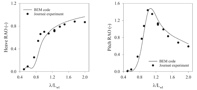
Fig. 5. Comparison between BEM code and results for Wigley III Journeé’s experimentation Fr = 0.2. |
For each of the 20,000 hulls, the first-order wave diffraction-radiation problem has been solved for 30 waves with wave lengths between 0.05Lwl and1.5Lwl, and for 7 incident wave directions between 0 and 180°. Froude-Krylov and wave diffraction loads haven been obtained for each wave frequency and direction. And added mass and damping matrices haven been obtained for each wave frequency.
Fig. 6 resumes the workflow strategy used to simulate the whole database of ships. Parametric variations of the parent's geometries have been carried out directly on the mesh generated for the base geometries.
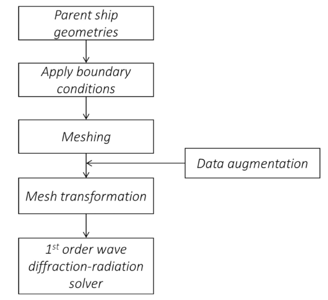
Fig. 6. Workflow for the seakeeping numerical simulation of the dataset of ships. |
For each parent geometry, a mesh sensitivity analysis has been carried out to ensure that convergence have been reached. Examples of the test carried out are presented here. Table 3, Table 4, Table 5, Table 6 shows a convergence analysis for three hull forms (the original and two extreme parametric variations B/D = 1.0 and L/B = 1.5), for four types of ships. Table 3, Table 4, Table 5, Table 6 provide the error differences computed between consecutive meshes for the normalized the diagonal terms of added mass, and damping matrices, and diffraction vector loads in percentage. From all those computed errors, the maximum is selected and shown in Table 3, Table 4, Table 5, Table 6. The meshes are noted by M capital letter, the refinement in number of panels is increased between meshes, so M i + 1 - M i shows error difference between them. Most of cases, mesh 1 has up to 200 panel, while mesh 8 reaches up to 10,000 panels. Fig. 7, Fig. 8, Fig. 9, Fig. 10 show the meshes analyzed. The error committed is less than 2% in most cases, when number of panels increases. The mesh selected is the number five.
Table 3. Mesh sensitivity analysis for container ship hull form. |
| Mesh diff. | Original | B/D = 1 | L/B = 1.5 | |||||||||
|---|---|---|---|---|---|---|---|---|---|---|---|---|
| Aii (%) | Bii (%) | fi (%) | mi (%) | Aii (%) | Bii (%) | fi (%) | mi (%) | Aii (%) | Bii (%) | fi (%) | mi (%) | |
| M 2 - M 1 | 1.41 | 2.39 | 0.45 | 0.10 | 0.13 | 0.59 | 0.13 | 0.00 | 2.20 | 2.86 | 6.90 | 0.73 |
| M 3 - M 2 | 0.94 | 0.32 | 0.53 | 0.03 | 0.76 | 2.52 | 0.41 | 0.03 | 9.26 | 7.62 | 7.02 | 0.80 |
| M 4 - M 3 | 1.00 | 0.76 | 0.10 | 0.01 | 0.17 | 0.33 | 0.03 | 0.00 | 8.67 | 5.96 | 7.92 | 0.82 |
| M 5 - M 4 | 0.64 | 0.45 | 0.21 | 0.00 | 0.54 | 1.38 | 0.14 | 0.00 | 1.47 | 2.13 | 1.01 | 0.11 |
| M 6 - M 5 | 0.15 | 0.15 | 0.09 | 0.00 | 0.17 | 0.68 | 0.09 | 0.01 | 0.57 | 0.63 | 1.06 | 0.10 |
| M 7 - M 6 | 0.35 | 0.17 | 0.06 | 0.00 | 0.09 | 0.16 | 0.00 | 0.00 | 0.39 | 0.52 | 0.65 | 0.07 |
| M 8 - M 7 | 0.76 | 0.35 | 0.21 | 0.02 | 0.52 | 0.67 | 0.13 | 0.00 | 1.16 | 1.55 | 2.15 | 0.18 |
Table 4. Mesh sensitivity analysis for cruise ship hull form. |
| Mesh diff. | Original | B/D = 1 | L/B = 1.5 | |||||||||
|---|---|---|---|---|---|---|---|---|---|---|---|---|
| Aii (%) | Bii (%) | fi (%) | mi (%) | Aii (%) | Bii (%) | fi (%) | mi (%) | Aii (%) | Bii (%) | fi (%) | mi (%) | |
| M 2 - M 1 | 0.76 | 0.33 | 1.01 | 0.02 | 0.10 | 0.05 | 0.03 | 0.00 | 2.48 | 0.66 | 0.12 | 0.01 |
| M 3 - M 2 | 7.60 | 0.79 | 1.58 | 0.11 | 3.38 | 18.54 | 1.69 | 0.14 | 8.77 | 9.16 | 19.44 | 2.26 |
| M 4 - M 3 | 0.40 | 0.18 | 0.30 | 0.01 | 0.15 | 0.08 | 0.01 | 0.00 | 0.74 | 0.26 | 0.10 | 0.00 |
| M 5 - M 4 | 7.16 | 2.27 | 2.09 | 0.41 | 0.28 | 0.42 | 0.10 | 0.00 | 0.81 | 7.58 | 7.96 | 0.90 |
| M 6 - M 5 | 2.71 | 1.44 | 2.02 | 0.27 | 0.20 | 0.31 | 0.04 | 0.00 | 1.26 | 7.43 | 4.89 | 0.38 |
| M 7 - M 6 | 5.57 | 1.47 | 1.78 | 0.26 | 0.04 | 0.14 | 0.02 | 0.00 | 2.13 | 2.30 | 2.41 | 0.15 |
| M 8 - M 7 | 2.99 | 0.50 | 0.57 | 0.11 | 0.41 | 0.42 | 0.09 | 0.00 | 2.35 | 1.54 | 1.75 | 0.08 |
Table 5. Mesh sensitivity analysis for tanker ship hull form. |
| Mesh diff. | Original | B/D = 1 | L/B = 1.5 | |||||||||
|---|---|---|---|---|---|---|---|---|---|---|---|---|
| Aii (%) | Bii (%) | fi (%) | mi (%) | Aii (%) | Bii (%) | fi (%) | mi (%) | Aii (%) | Bii (%) | fi (%) | mi (%) | |
| M 2 - M 1 | 0.32 | 0.20 | 0.11 | 0.00 | 2.01 | 0.71 | 0.09 | 0.00 | 0.36 | 2.36 | 0.34 | 0.04 |
| M 3 - M 2 | 0.33 | 0.13 | 0.06 | 0.00 | 0.02 | 0.10 | 0.02 | 0.00 | 0.08 | 0.06 | 0.03 | 0.00 |
| M 4 - M 3 | 0.05 | 0.14 | 0.07 | 0.00 | 0.18 | 0.07 | 0.01 | 0.00 | 0.06 | 0.55 | 0.13 | 0.02 |
| M 5 - M 4 | 0.56 | 0.20 | 0.06 | 0.00 | 0.05 | 0.17 | 0.01 | 0.00 | 0.12 | 0.03 | 0.02 | 0.00 |
| M 6 - M 5 | 0.09 | 0.06 | 0.05 | 0.00 | 0.08 | 0.08 | 0.03 | 0.00 | 0.11 | 0.31 | 0.05 | 0.00 |
| M 7 - M 6 | 0.23 | 0.21 | 0.15 | 0.02 | 0.10 | 0.17 | 0.05 | 0.01 | 0.13 | 0.38 | 0.19 | 0.02 |
| M 8 - M 7 | 0.10 | 0.10 | 0.01 | 0.00 | 0.18 | 0.03 | 0.01 | 0.00 | 0.06 | 0.30 | 0.06 | 0.01 |
Table 6. Mesh sensitivity analysis for frigate ship hull form. |
| Mesh diff. | Original | B/D = 1 | L/B = 1.5 | |||||||||
|---|---|---|---|---|---|---|---|---|---|---|---|---|
| Aii (%) | Bii (%) | fi (%) | mi (%) | Aii (%) | Bii (%) | fi (%) | mi (%) | Aii (%) | Bii (%) | fi (%) | mi (%) | |
| M 2 - M 1 | 6.46 | 2.61 | 1.29 | 0.07 | 1.79 | 2.79 | 0.73 | 0.05 | 5.34 | 8.16 | 2.76 | 0.20 |
| M 3 - M 2 | 3.30 | 0.37 | 0.45 | 0.03 | 0.49 | 0.20 | 0.09 | 0.00 | 0.60 | 0.34 | 0.58 | 0.06 |
| M 4 - M 3 | 0.20 | 0.12 | 0.16 | 0.00 | 0.24 | 0.25 | 0.10 | 0.00 | 0.07 | 0.14 | 0.15 | 0.01 |
| M 5 - M 4 | 0.47 | 0.60 | 0.24 | 0.01 | 0.19 | 0.08 | 0.04 | 0.00 | 0.27 | 0.14 | 0.36 | 0.03 |
| M 6 - M 5 | 0.60 | 0.22 | 0.29 | 0.01 | 0.55 | 0.41 | 0.19 | 0.01 | 0.16 | 0.19 | 0.19 | 0.02 |
| M 7 - M 6 | 0.15 | 0.10 | 0.04 | 0.00 | 0.02 | 0.01 | 0.01 | 0.00 | 0.04 | 0.02 | 0.06 | 0.01 |
| M 8 - M 7 | 0.55 | 0.31 | 0.11 | 0.01 | 0.36 | 0.54 | 0.07 | 0.00 | 0.08 | 0.07 | 0.17 | 0.01 |
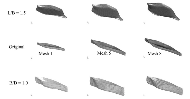
Fig. 7. Caption with three different meshes of a container parent ship. |
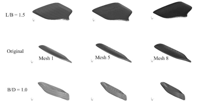
Fig. 8. Caption with three different meshes of a cruise parent ship. |
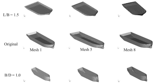
Fig. 9. Caption with three different meshes of a tanker parent ship. |
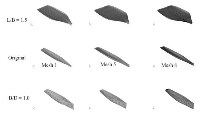
Fig. 10. Caption with three different meshes of a frigate parent ship. |
4.3. ANN inputs and targeted outputs
In the early stages of the design of a ship, the exact hull geometry is unknown, and this is needed to predict the seakeeping particulars using numerical simulations or model testing. However, main particulars of the ship geometry, as the length, beam, draft, and form coefficient can be bounded within a range based on similar ships.
The objective of this work is to obtain a fast and accurate AI algorithm capable of predicting the seakeeping particulars of a conventional monohull ship, so that could be used to predict the seakeeping performance in the early stage of design. And since the exact geometry is not known, the AI should be based on the ship´s geometry main particulars.
ANN inputs identification is a key point to enable the ANN to predict how changes in the hull geometry modify the seakeeping outputs. We define the ANN seakeeping target outputs as: the added mass and damping matrices, and the excitation loads for all six degrees of freedom. And these targets (ti) are assumed to mainly depend on the main dimensionless form factors of the hull geometry [29,30].
$ t_{i}=f\left(\frac{\mathrm{B}_{\mathrm{wl}}}{\mathrm{L}_{\mathrm{wl}}}, \frac{\mathrm{D}}{\mathrm{L}_{\mathrm{wl}}}, C_{\mathrm{b}}, C_{\mathrm{wl}}, C_{\mathrm{m}}, C_{\mathrm{c}}, \frac{\mathrm{X}_{\mathrm{B}}}{\mathrm{L}_{\mathrm{wl}}}, \frac{\mathrm{Z}_{\mathrm{B}}}{\mathrm{D}}\right), $
where Lwl is the waterline length, Bwl is the maximum waterline beam, D is the draft, Cb is the block coefficient, Cwl is the waterplane coefficient, Cm is the midship coefficient, Cc is the amidships coefficient, and XB and ZB are the longitudinal and vertical position of the buoyancy center, respectively.
For each nonzero component of the added mass and damping matrices, an ANN is built. An ANN is also built for every component of the excitation loads and wave heading. And 70% of the database of ships is used for the training, while 15% is used for the validation and the other 15% is used for the test.
5. Predictive algorithm
In this section, the process carried out to select the best ANN is presented. The selected ANN will be the one that minimize the prediction error. The Multi-Layer Perceptron (MLP) [9,10] model has been used for the regression problem. Tensorflow 2.1.0 [31] along with GPU Nvidia acceleration libraries [32] have been used for the ANN development. GPU architecture are capable of speeding up the training process, achieving training times up to 10 times faster when compared to CPU architectures [9].
In order to obtain an optimal ANN architecture, a large number of ANNs with different parameters and hyper-parameters are trained and verified. Then, the errors are compared to select the best one. Eq. (1) provides a formulation for the mean absolute error (MAE) used [33⇓⇓-36], where ti is the value obtained by numerical simulation, pi is the ANN predicted value, and n is the total number of parameters. And Table 7 shows the parametric variation carried out to generate the different ANN architectures.
$ MAE=\frac{\sum_{i=1}^{n}\left|t_{i}-p_{i}\right|}{n} $
Table 7. Parametric variation of ANN architecture hyper-parameters. |
| Hyper-parameter | Variation |
|---|---|
| Number of hidden layers | 1-2-3 |
| Number of neurons per hidden layer | 10-20-30-40 |
| Optimization algorithms | Adam [37] RMSprop [38] models |
| Activation functions for each layer | Sigmoid [39] ReLU [40,41] |
| Number of training epochs | ∈ [100, 300] |
| Overfitting prevention | Batch Normalization [42] Dropout [43,44] Regularization functions L1 [45] Regularization function L2 [46] |
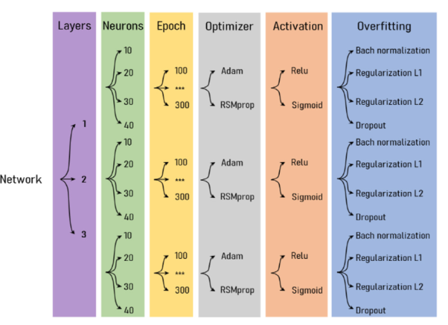
Fig. 11. Graphic representation for the ANN architectures generated by parametric variations of hyper-parameters. |
Fig. 12 shows the competition process applied to select best ANN to predict the added mass in heave (a33). Each ANN (individual point in Fig. 12) is trained with a combination of the hyper-parameters from 1 to 5 (see Table 7). The best combination comes from the minimization of the MAE. Pareto front shows the minimum MAEs in the first step of the competition process applied to different number of neurons and layers. Then, overfitting prevent techniques (dropout), batch normalization, and regularization are applied, in next two septs, to those points having minimum MAE. In second step, dropout techniques are applied in those winner architectures from the first step. Then, in step three, the combinations of hyperparameters with lowest MAE are tested with batch normalization and regularization techniques.
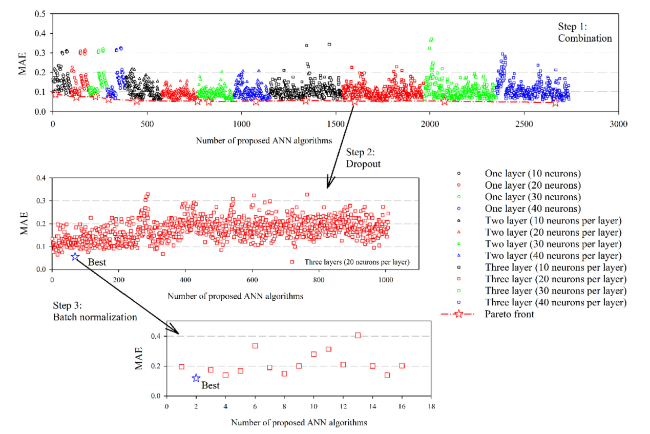
Fig. 12. MAE versus number of neurons and layers. |
After applying the three training steps shown in Fig. 12, the ANN with the lowest MAE is selected. It is worth mentioning that steps 2 and 3 do not always improve on the training performed in step 1. Fig. 12 shows an example of this, where the best ANN had been trained in the first step of the process.
From the training process it can be concluded that one layer is not enough to reach fitted predictions. Increasing the number of layers from one to two, the curves fitting improves up to 25%, and the increasing from two to three the gain is up to 15% additional. It should be noted, that the greater number of layers the greater risk of overfitting.
As for the number of neurons per layer, using 30 neurons fitted predictions are achieved with MAE errors below 5%. And it is observed that the Adam optimizer provides better results than the RMSprop. Furthermore, the results improve when the two activation functions are included in the ANN.
6. Numerical assessment and computational performance
6.1. Numerical assessment
This work focuses on predicting almost instantly the seakeeping loads for a wide range of conventional monohull ships. This range includes crude carriers, container ships, supply vessels, and many others as reported in Section 6.
To demonstrate the validity ANNs developed, five assessment cases are computed and compared to the results obtained by the BEM code used to generate the target outputs of the ANNs. This inter-code comparison is carried for five hull geometries different to those of the parent ships database. Fig. 13 compares the dimensionless form factor for the parent ships database and the assessment cases. Table 8 provides the main hull form parameters as well as their typology and Fig. 14 shows sections and 3D views for the assessment cases.
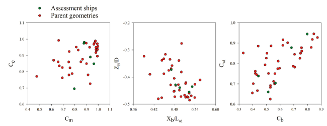
Fig. 13. Dimensionless ship form parameters for the parent ships used for the trainings and the five assessment ships. |
Table 8. Main dimensionless hull parameters for the five assessment ships. |
| Assessment test | Typology | $ \frac{\mathrm{B}_{\mathrm{wl}}}{\mathrm{L}_{\mathrm{wl}}} $ | $ \frac{D}{\mathrm{~L}_{\mathrm{wl}}} $ | Cb | Cwl | Cm | Cp | $ \frac{\mathrm{X}_{\mathrm{B}}}{\mathrm{L}_{\mathrm{wl}}} $ | $ \frac{Z_{B}}{D} $ |
|---|---|---|---|---|---|---|---|---|---|
| 1 | Anchor Handling | 0.286 | 0.100 | 0.683 | 0.878 | 0.963 | 0.710 | 0.495 | −0.439 |
| 2 | Landing craft | 0.318 | 0.036 | 0.798 | 0.945 | 0.933 | 0.855 | 0.523 | −0.455 |
| 3 | Trawler | 0.257 | 0.060 | 0.513 | 0.660 | 0.881 | 0.582 | 0.483 | −0.429 |
| 4 | Yacht | 0.230 | 0.034 | 0.441 | 0.739 | 0.796 | 0.554 | 0.470 | −0.372 |
| 5 | Container ship | 0.140 | 0.048 | 0.566 | 0.704 | 0.878 | 0.646 | 0.532 | −0.435 |
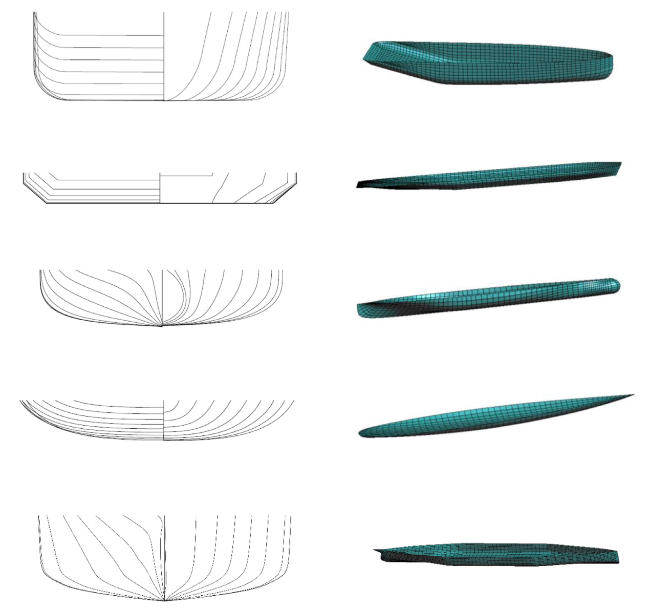
Fig. 14. Hull shapes below waterline for the five tests. Left: Body plan; Right: 3D view. |
Appendices B - E show graphical comparisons of the results obtained for ANNs versus BEM. The dimensionless diagonal values of the added mass and damping matrices are compared for different wavelengths. In addition, results of excitation loads for 7 headings and RAOs for 3 headings (0, 30, and 60°) are also compared.
6.2. Computational performance
One of the objectives of this work is to develop an AI capable of predicting seakeeping wave loads so that this AI can be used in the early stages of the ship design. Then, this tool should be capable of making fast predictions that can be used iteratively within the ship design process.
One of the main advantages of ANNs is that, once they have been trained and calibrated, they can compute complex problems almost immediately. In the case of this work, it is expected that seakeeping wave loads for a conventional monohull ship can be obtained much faster than using a traditional BEM code. And equally important, without the need of the exact hull geometry and the corresponding computational mesh.
Fig 15 shows the computational time required for computing all the seakeeping loads for 6000 hulls, including the computational time for reading the input file, carrying out the ANN computation, and writing all the outputs. For each of those cases, 30 wave frequencies and 7 wave directions are considered. This experiment was carried out with a computer with the following particulars:
- CPU: AMD Ryzen 7 3700 × 8 core Processor.
- GPU: Nvidia GeForce RTX2060.
- RAM: 32 GB.
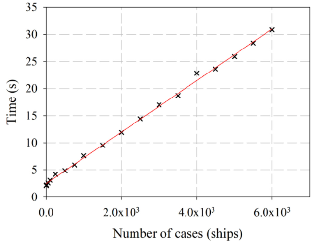
Fig. 15. Computational time in seconds versus number of cases computed. |
It is observed that the computational velocity is about 200 cases/second. Given this computing velocity, and optimization algorithm based on a systematic variation of the ship form parameters could be used in the early design of a ship.
7. Results discussion
The fitting of an ANNs curve to a BEM curve is measured by the Mean Normalized Relative Error (MNRE) defined as follows,
$ N R E_{i}=\frac{\left|t_{i}^{*}-p_{i}^{*}\right|}{\max \left(1,\left|t_{i}\right|\right)} $
$ M N R E=\sqrt{\frac{\sum_{i=1}^{n} N R E_{i}{ }^{2}}{n}}, $
being NREi the normalized error in a point i, ti* the dimensionless target,pi* the dimensionless prediction, and n the number of curve points.
Table 9. Normalized relative mean error for predicted dimensionless added masses. |
| MNRE (%) | a11* | a22* | a33* | a44* | a55* | a66* | Average |
|---|---|---|---|---|---|---|---|
| Anchor Handling | 0.35 | 4.44 | 4.45 | 4.34 | 4.17 | 3.26 | 3.50 |
| Landing craft | 0.58 | 1.13 | 1.47 | 12.02 | 3.40 | 1.58 | 3.36 |
| Trawler | 0.20 | 4.01 | 3.18 | 4.62 | 3.18 | 4.84 | 3.34 |
| Yacht | 0.19 | 4.14 | 4.21 | 6.05 | 1.68 | 0.97 | 2.87 |
| Container ship | 0.24 | 5.50 | 5.33 | 5.99 | 7.25 | 3.93 | 4.71 |
| Average | 0.31 | 3.84 | 3.73 | 6.61 | 3.94 | 2.92 | 3.56 |
Table 10. Normalized relative mean error for predicted dimensionless dampings. |
| MNRE (%) | b11* | b22* | b33* | b44* | b55* | b66* | Average |
|---|---|---|---|---|---|---|---|
| Anchor Handling | 0.38 | 6.07 | 1.26 | 0.73 | 3.93 | 6.77 | 3.19 |
| Landing craft | 0.23 | 1.87 | 5.89 | 13.14 | 6.40 | 1.04 | 4.76 |
| Trawler | 0.43 | 3.75 | 1.76 | 2.27 | 4.77 | 5.16 | 3.02 |
| Yacht | 0.24 | 1.04 | 5.25 | 7.05 | 7.12 | 0.44 | 3.52 |
| Container ship | 0.31 | 2.44 | 3.95 | 3.28 | 4.10 | 1.84 | 2.65 |
| Average | 0.32 | 3.03 | 3.62 | 5.30 | 5.27 | 3.05 | 3.43 |
Fig. D.1 shows the dimensionless excitation loads (sum of the diffraction and the Froude-Krylov loads) for surge (f11*) and pitch (my*). It is compared for seven headings and four wavelengths. The MNRE values for the excitation forces are shown in Tables F.1 to F.5. The average value for predicter forces goes from 1.78 to 3.28%. The largest deviations are observed for pitch moments with wave headings closed to the ship's transversal direction.
Figs. E.1-E.5 show the RAOs for heave, roll and pitch for 0, 30, and 60° headings. Tables G.1-G.5 provide MNRE values for the heave, roll, and pitch RAO curves. The average difference between curves ranges from 1.34% to 3.38%. Let's point out that RAO curves are not directly predicted by ANN, but obtained from postprocessing the ANN results along with ships particulars such as position of the gravity center, and the mass and inertia matrix.
In general, the prediction of dimensionless added masses and damping values is better than those for the excitation loads. As a first approach, in this work it was assumed that optimizing an ANN for the added masses in heave (a33) would predict well the other outputs. This was assumed to reduce the large number of combinations given to solve full ANN optimization problem, leading to train millions of ANNs. Also, it is observed that trained ANNs naturally remove the irregular frequencies typically obtained from BEM codes, improving the targeted outputs.
8. Conclusions
This work demonstrate that algorithms based on ANNs could be suitable to predict the seakeeping loads needed to include seakeeping in early design stages of conventional monohulls ships. A large database and widespread has been used to achieve an accurate ANN. Starting from a database of 50 parent ships (see Table A1), data augmentation technique was used to increase the number of hulls up to 20,000. This augmentation was based on systematic geometric variations of the parent ships. Then, a BEM solver was used to compute a large output for training the ANNs.
One of the main achievements of this work is to obtain an AI algorithm capable of predict the seakeeping loads acting on a ship with no need of the exact geometry of the hull. Instead basic hull form coefficients, used in the early design, are required. And the generated algorithm will be able to predict the seakeeping particulars of any conventional monohull ship whose shape coefficients are within the limits shown in Table 1.
A competitive process has been proposed to select best combination of hyper-parameters. Then a set of ANNs capable of predict different components of the seakeeping loads have been obtained.
In this work it has been demonstrated the potential of ANNs to fast computation of seakeeping loads achieving more than 200 ships per second. Moreover, the ANNs can naturally remove irregular output data computed by BEM solvers.
Declaration of Competing Interest
The authors declare that they have no known competing financial interests or personal relationships that could have appeared to influence the work reported in this paper.
Appendix A
Table A1. Parent ships. |
| Number of ships | Type | L/B | B/D | Cb | Fr |
|---|---|---|---|---|---|
| 1 | Cargo Ship | 4.492 | 2.500 | 0.56 | 0.322 |
| 2 | Tugboat | 3.233 | 2.284 | 0.50 | 0.454 |
| 3 | Bulk carrier | 6.753 | 2.311 | 0.75 | 0.171 |
| 4 | Bulk carrier | 6.389 | 3.852 | 0.74 | 0.186 |
| 5 | Container ship | 6.644 | 2.538 | 0.55 | 0.275 |
| 6 | Container ship | 6.235 | 4.125 | 0.53 | 0.259 |
| 7 | Supply vessel | 4.013 | 2.839 | 0.53 | 0.610 |
| 8 | Supply vessel | 4.757 | 4.457 | 0.33 | 0.652 |
| 9 | Cruise ship | 8.432 | 4.386 | 0.60 | 0.191 |
| 10 | Cruise ship | 7.825 | 6.351 | 0.58 | 0.238 |
| 11 | Tanker ship | 5.951 | 2.714 | 0.87 | 0.131 |
| 12 | Drill ship | 5.951 | 4.750 | 0.84 | 0.153 |
| 13 | FPSO | 5.858 | 4.521 | 0.83 | 0.129 |
| 14 | harbor tug | 2.922 | 2.607 | 0.62 | 0.342 |
| 15 | harbor tug | 2.362 | 3.861 | 0.66 | 0.307 |
| 16 | Heave lift ship | 3.657 | 5.556 | 0.85 | 0.158 |
| 17 | Patrol vessel | 5.902 | 2.855 | 0.49 | 0.474 |
| 18 | Patrol vessel | 6.156 | 4.503 | 0.40 | 0.452 |
| 19 | Cargo vessel | 5.860 | 2.250 | 0.71 | 0.240 |
| 20 | Cargo vessel | 5.520 | 3.374 | 0.71 | 0.304 |
| 21 | Frigate | 6.347 | 3.159 | 0.51 | 0.514 |
| 22 | Frigate | 6.003 | 6.022 | 0.40 | 0.541 |
| 23 | Ro-On Ro-Off | 7.063 | 4.127 | 0.53 | 0.234 |
| 24 | Supply vessel | 3.640 | 2.566 | 0.62 | 0.411 |
| 25 | Yacht | 4.806 | 2.947 | 0.42 | 0.325 |
| 26 | Yacht | 9.163 | 3.215 | 0.43 | 0.299 |
| 27 | Yacht | 6.253 | 3.165 | 0.42 | 0.457 |
| 28 | Benchmark hull | 10.000 | 1.587 | 0.43 | 0.250 |
| 29 | Cargo ship | 2.482 | 5.034 | 0.59 | 0.234 |
| 30 | Container ship | 3.644 | 3.703 | 0.53 | 0.265 |
| 31 | Container ship | 7.042 | 2.659 | 0.56 | 0.305 |
| 32 | Cargo vessel | 5.701 | 2.690 | 0.70 | 0.281 |
| 33 | Yacht | 3.526 | 2.304 | 0.44 | 0.346 |
| 34 | Cargo vessel | 6.667 | 2.312 | 0.76 | 0.220 |
| 35 | Yacht | 6.250 | 2.158 | 0.50 | 0.348 |
| 36 | LNG ship | 6.187 | 4.104 | 0.76 | 0.187 |
| 37 | Bulk carrier | 6.771 | 1.926 | 0.77 | 0.194 |
| 38 | Bulk carrier | 6.459 | 2.992 | 0.79 | 0.202 |
| 39 | Supply vessel | 4.077 | 3.455 | 0.47 | 0.681 |
| 40 | Container ship | 6.545 | 2.198 | 0.59 | 0.292 |
| 41 | Container ship | 6.185 | 5.077 | 0.61 | 0.309 |
| 42 | Drill ship | 5.838 | 3.455 | 0.87 | 0.138 |
| 43 | Drill ship | 6.326 | 5.833 | 0.89 | 0.160 |
| 44 | FPSO | 5.728 | 9.042 | 0.81 | 0.159 |
| 45 | harbor tug | 3.862 | 1.714 | 0.61 | 0.308 |
| 46 | Patrol vessel | 6.606 | 3.289 | 0.37 | 0.469 |
| 47 | Cargo vessel | 6.489 | 3.783 | 0.76 | 0.279 |
| 48 | Cargo vessel | 5.203 | 1.798 | 0.74 | 0.265 |
| 49 | Frigate | 6.389 | 4.174 | 0.45 | 0.523 |
| 50 | Frigate | 6.123 | 2.086 | 0.45 | 0.579 |
Appendix B
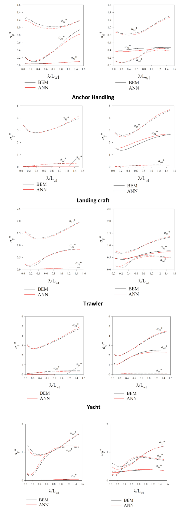
Fig. B.1. Added mass comparison between ANN and BEM for the five assessment ships. |
Appendix C
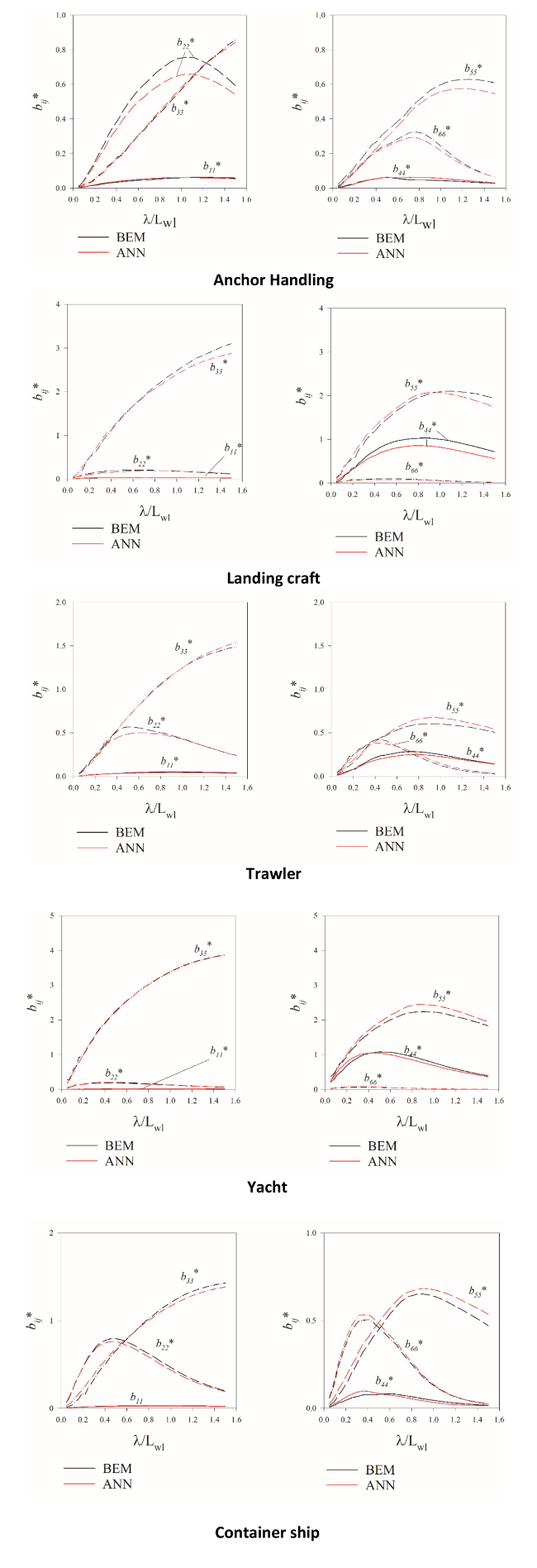
Fig. C.1. Damping comparison between ANN and BEM for the five assessment ships. |
Appendix D
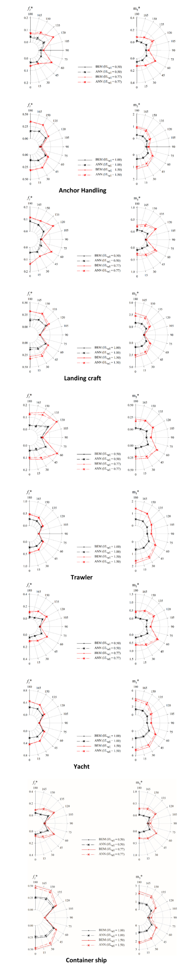
Fig. D.1. Wave excitation loads comparison between ANN and BEM for the five assessment ships. |
Appendix E
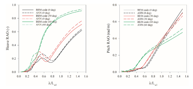
Fig. E.1. Heave and Pitch RAO comparisons between ANN and BEM for the container assessment ship. |
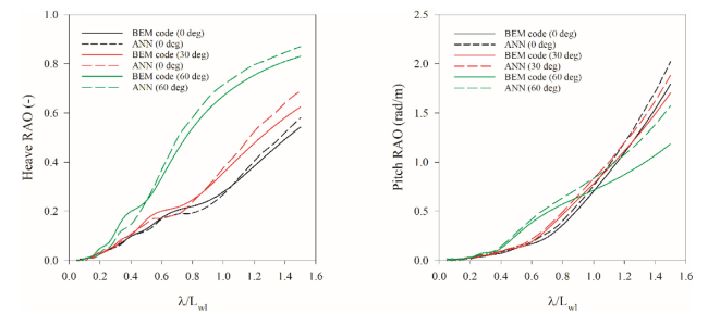
Fig. E.2. Heave and Pitch RAO comparisons between ANN and BEM for the yacht assessment ship. |
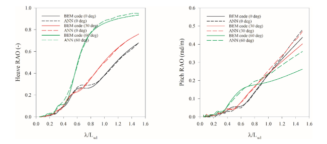
Fig. E.3. Heave and Pitch RAO comparisons between ANN and BEM for the Trawler assessment ship. |
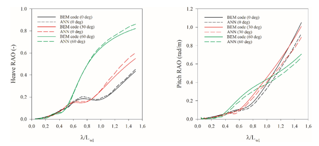
Fig. E.4. Heave and Pitch RAO comparisons between ANN and BEM for the Landing craft assessment ship. |
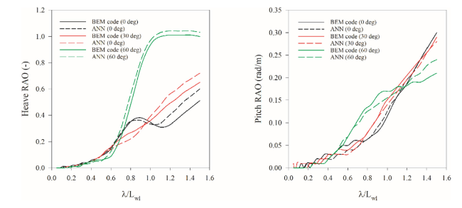
Fig. E.5. Heave and Pitch RAO comparisons between ANN and BEM for the anchor handling assessment ship. |
Appendix F
Table F.1. Assessment ship 1 (Anchor Handling): MNRE for excitation loads. |
| Heading | 0° | 30° | 60° | 90° | 120° | 150° | 180° | Average | |
|---|---|---|---|---|---|---|---|---|---|
| MNRE [%] | fx | 1.27 | 0.47 | 0.89 | 1.71 | 0.46 | 0.69 | 1.01 | 0.93 |
| fy | 0.01 | 1.58 | 2.19 | 9.36 | 4.21 | 1.61 | 0.01 | 2.71 | |
| fz | 2.88 | 2.37 | 1.37 | 1.29 | 2.72 | 2.34 | 1.36 | 2.05 | |
| mx | 0.01 | 2.67 | 11.59 | 7.50 | 4.02 | 4.06 | 0.01 | 4.27 | |
| my | 5.18 | 6.53 | 2.60 | 2.87 | 4.26 | 3.96 | 2.98 | 4.05 | |
| mz | 0.01 | 0.92 | 1.71 | 0.50 | 1.23 | 2.44 | 0.01 | 0.97 | |
| Average | 1.56 | 2.43 | 3.39 | 3.87 | 2.82 | 2.52 | 0.90 | 2.50 | |
Table F.2. Assessment ship 2 (Landing craft): MNRE for excitation loads. |
| Heading | 0° | 30° | 60° | 90° | 120° | 150° | 180° | Average | |
|---|---|---|---|---|---|---|---|---|---|
| MNRE [%] | fx | 3.43 | 2.57 | 0.51 | 0.27 | 1.63 | 1.04 | 1.54 | 1.57 |
| fy | 0.01 | 0.51 | 1.04 | 1.53 | 2.16 | 1.10 | 0.01 | 0.91 | |
| fz | 1.57 | 1.17 | 2.10 | 1.51 | 2.78 | 1.77 | 4.71 | 2.23 | |
| mx | 0.01 | 2.05 | 6.12 | 11.18 | 1.99 | 2.65 | 0.01 | 3.43 | |
| my | 7.76 | 7.84 | 7.72 | 0.70 | 6.25 | 8.22 | 9.21 | 6.81 | |
| mz | 0.01 | 0.94 | 1.52 | 0.21 | 1.56 | 0.29 | 0.01 | 0.65 | |
| Average | 2.13 | 2.51 | 3.17 | 2.57 | 2.73 | 2.51 | 2.58 | 2.60 | |
Table F.3. Assessment ship 3 (Trawler): MNRE for excitation loads. |
| Heading | 0° | 30° | 60° | 90° | 120° | 150° | 180° | Average | |
|---|---|---|---|---|---|---|---|---|---|
| MNRE [%] | fx | 0.98 | 1.33 | 0.47 | 0.51 | 0.50 | 1.61 | 0.50 | 0.84 |
| fy | 0.01 | 1.72 | 3.32 | 2.19 | 4.52 | 1.20 | 0.01 | 1.85 | |
| fz | 1.36 | 1.19 | 1.98 | 2.00 | 1.83 | 1.99 | 2.02 | 1.77 | |
| mx | 0.01 | 4.58 | 2.76 | 2.54 | 4.16 | 6.27 | 0.01 | 2.90 | |
| my | 5.71 | 4.13 | 2.48 | 1.23 | 1.01 | 1.62 | 1.86 | 2.58 | |
| mz | 0.01 | 0.76 | 0.80 | 1.69 | 0.96 | 0.78 | 0.01 | 0.71 | |
| Average | 1.35 | 2.29 | 1.97 | 1.69 | 2.16 | 2.24 | 0.74 | 1.78 | |
Table F.4. Assessment ship 4 (Yatch): MNRE for excitation loads. |
| Heading | 0° | 30° | 60° | 90° | 120° | 150° | 180° | Average | |
|---|---|---|---|---|---|---|---|---|---|
| MNRE [%] | fx | 0.71 | 0.32 | 0.38 | 0.28 | 0.96 | 0.34 | 0.77 | 0.54 |
| fy | 0.01 | 3.28 | 1.98 | 0.86 | 5.45 | 3.83 | 0.01 | 2.20 | |
| fz | 3.33 | 3.94 | 4.24 | 2.95 | 3.48 | 2.34 | 3.11 | 3.34 | |
| mx | 0.01 | 8.38 | 5.48 | 3.21 | 5.61 | 8.31 | 0.01 | 4.43 | |
| my | 4.24 | 6.29 | 4.66 | 0.74 | 7.14 | 6.35 | 5.79 | 5.03 | |
| mz | 0.01 | 0.72 | 0.36 | 0.61 | 0.53 | 0.52 | 0.01 | 0.39 | |
| Average | 1.38 | 3.82 | 2.85 | 1.44 | 3.86 | 3.62 | 1.62 | 2.66 | |
Table F.5. Assessment ship 5 (Container ship): MNRE for excitation loads. |
| Heading | 0° | 30° | 60° | 90° | 120° | 150° | 180° | Average | |
|---|---|---|---|---|---|---|---|---|---|
| MNRE [%] | fx | 1.74 | 2.29 | 1.53 | 1.43 | 1.84 | 1.85 | 1.62 | 1.76 |
| fy | 0.01 | 1.57 | 1.82 | 1.01 | 2.98 | 1.23 | 0.01 | 1.23 | |
| fz | 2.63 | 3.95 | 1.90 | 2.25 | 1.41 | 1.07 | 2.49 | 2.24 | |
| mx | 0.01 | 8.25 | 16.08 | 14.37 | 6.59 | 4.94 | 0.01 | 7.18 | |
| my | 4.48 | 4.09 | 2.38 | 16.53 | 4.43 | 5.91 | 6.24 | 6.29 | |
| mz | 0.10 | 0.99 | 0.32 | 4.54 | 0.47 | 0.29 | 0.01 | 0.96 | |
| Average | 1.50 | 3.52 | 4.01 | 6.69 | 2.95 | 2.55 | 1.73 | 3.28 | |
Appendix G
Table G.1. Assessment ship 1 (Anchor Handling): MNRE for RAO. |
| Heading | 0° | 30° | 60° | 90° | 120° | 150° | 180° | Average | |
|---|---|---|---|---|---|---|---|---|---|
| MNRE [%] | RAO33 | 3.76 | 3.47 | 3.31 | 2.43 | 3.42 | 2.63 | 1.76 | 2.97 |
| RAO44 | 0.28 | 0.13 | 0.22 | 0.24 | 0.22 | 0.16 | 0.00 | 0.18 | |
| RAO55 | 0.79 | 0.69 | 1.23 | 1.38 | 0.79 | 0.58 | 0.63 | 0.87 | |
| Average | 1.61 | 1.43 | 1.59 | 1.35 | 1.48 | 1.12 | 0.79 | 1.34 | |
Table G.2. Assessment ship 2 (Landing craft): MNRE for RAO. |
| Heading | 0° | 30° | 60° | 90° | 120° | 150° | 180° | Average | |
|---|---|---|---|---|---|---|---|---|---|
| MNRE [%] | RAO33 | 0.96 | 1.90 | 1.37 | 2.36 | 1.58 | 1.07 | 1.59 | 1.55 |
| RAO44 | 0.00 | 0.50 | 1.88 | 2.89 | 1.23 | 0.58 | 0.00 | 1.01 | |
| RAO55 | 4.45 | 4.54 | 2.98 | 2.56 | 3.76 | 5.39 | 6.56 | 4.32 | |
| Average | 1.81 | 2.31 | 2.08 | 2.61 | 2.19 | 2.35 | 2.72 | 2.29 | |
Table G.3. Assessment ship 3 (Trawler): MNRE for RAO. |
| Heading | 0° | 30° | 60° | 90° | 120° | 150° | 180° | Average | |
|---|---|---|---|---|---|---|---|---|---|
| MNRE [%] | RAO33 | 1.05 | 0.67 | 1.72 | 1.90 | 1.15 | 2.27 | 2.07 | 1.55 |
| RAO44 | 0.00 | 0.25 | 0.53 | 1.21 | 0.79 | 0.21 | 0.00 | 0.43 | |
| RAO55 | 1.34 | 2.14 | 3.77 | 5.88 | 2.10 | 0.69 | 1.34 | 2.47 | |
| Average | 0.80 | 1.02 | 2.01 | 3.00 | 1.35 | 1.06 | 1.14 | 1.48 | |
Table G.4 Assessment ship 4 (Yatch): MNRE for RAO. |
| Heading | 0° | 30° | 60° | 90° | 120° | 150° | 180° | Average | |
|---|---|---|---|---|---|---|---|---|---|
| MNRE [%] | RAO33 | 1.41 | 2.57 | 3.47 | 1.64 | 2.76 | 1.86 | 2.40 | 2.30 |
| RAO44 | 0.00 | 0.37 | 0.83 | 1.86 | 1.53 | 0.51 | 0.00 | 0.73 | |
| RAO55 | 5.29 | 4.16 | 12.21 | 8.40 | 6.92 | 6.85 | 5.97 | 7.11 | |
| Average | 2.23 | 2.37 | 5.50 | 3.97 | 3.74 | 3.07 | 2.79 | 3.38 | |
Table G.5. Assessment ship 5 (Container ship): MNRE for RAO. |
| Heading | 0° | 30° | 60° | 90° | 120° | 150° | 180° | Average | |
|---|---|---|---|---|---|---|---|---|---|
| MNRE [%] | RAO33 | 2.69 | 3.81 | 2.92 | 2.85 | 2.13 | 0.88 | 2.68 | 2.57 |
| RAO44 | 0.00 | 0.12 | 0.39 | 0.48 | 0.38 | 0.18 | 0.00 | 0.22 | |
| RAO55 | 1.92 | 1.62 | 1.96 | 6.73 | 1.75 | 2.32 | 2.61 | 2.70 | |
| Average | 1.54 | 1.85 | 1.76 | 3.35 | 1.42 | 1.13 | 1.76 | 1.83 | |
