
1. Introduction
In order to design maritime structures ranging from wharfs to oil rigs, it is important to estimate the wave climate and the extreme values, as well as to evaluate the impacts of possible future climate change [1,2]. Performing extreme analysis on time series of wave data, such as in situ measurements, satellite estimates, or numerical model results, can provide an assessment of possible rare events [3,4]. In this regard, a review of statistical models for extreme events was conducted by Jonathan and Ewans, to assist the design of marine structures [5]. Although stochastic methods are able to estimate extreme values of return periods for time-series, application of these methods to extensive geographical areas, using numerical models with time-series in each computational element in space may be overwhelming [6,7]. Complex coupled ocean-atmosphere model systems, long records of observed data, large datasets of remotely sensed satellite observations, and high-resolution numerical model outputs can potentially lead to unmanageably huge datasets [8⇓⇓-11]. Moreover, stochastic methods can be applied to assess wave regimes over large geographical study areas, including parameters such as significant wave heights (Hs), mean wave periods (T0), and mean wave directions (MWD). Data mining tools may be used to facilitate data analysis, including redundancy, and classification of areas of high rates of similarity [12,13]. More specifically, spatial data mining methods can be applied to identify spatial features, patterns and relationships [14,15]. For this purpose, techniques to classify and cluster have become well-developed scientific tools [16,17] permitting the division of data into categories with similar characteristics [18].
However, although there are a variety of different clustering methods, application of these techniques to spatial time-series data have faced several challenges, due to the variations in time and space. Thus, the idea of spatial clustering was proposed to categorize the scatter of spatial data into classes, with maximal resemblance, optimizing the degree of uniformity. In order to move forward with this concept, a number of methodologies have been generated, such as k-means, density-based spatial clustering of applications with noise, self-organizing maps (SOMs), etc. [19⇓⇓⇓-23]. Nevertheless, most of these require considerable improvement to determine spatial patterns, including neighbors, in order to be applicable as clustering methods [24]. To cope with the issues of spatial clustering, unsupervised artificial neural networks, or SOMs, have been applied to a wide variety of spatial data [25].
As an unsupervised neural network, the Self-Organizing Map (SOM) methodology, also known as Kohonen Map or Self-Organizing Feature Map, is a competitive learning technique [26,27]. The spatial version of SOM is presented by Bação et al., [28,29]. A specific inter-relatedness of spatial dimensions and the significance of this sub-space in a geographer's analyses can be identified by GeoSOM [30]. Taking Tobler's First Law into consideration, GeoSOM investigates clusters within identical geographic boundaries, instead of global clusters produced by standard SOM methodologies. Applying the SOM technique or other associated methods in oceanography was initially restricted to remote-sensing data, and in situ biological/geochemical analyses data [31⇓⇓⇓⇓⇓-37]. Moreover, in recent years, application of SOM clustering techniques has been increasingly developed in other areas of oceanography [38⇓⇓-41]. Employing this approach to identify patterns in oceanographic data, including ocean currents, sea surface heights, sea surface temperature, satellite ocean color, chlorophyll, etc. can lead to remarkable results [42⇓⇓-45].
A powerful unsupervised clustering method resulting from the SOM methodology is called the neural gas (NG) method. Martinetz and Schulten (1991) introduced the NG algorithm, which is an artificial neural network inspired by SOM [46]. The NG algorithm determines the optimal data representations according to feature vectors. The name for this algorithm is taken from the dynamics of the feature vectors during the adaptation process, which distribute themselves like a gas within the data space. This technique has wide application in image processing or pattern recognition [47,48].
Although clustering techniques based on artificial neural networks fail to take extreme or rare events into consideration, for example maximum values for Hs to T0 over a long time period, there are important benefits to these methods, such as unsupervised learning, and provision of multidimensional knowledge from a two-dimensional lattice. Thus, SOMs have become categorized as among preferable clustering methods [49]. Moreover, adaptations have been applied to allow consideration of maximum values in a time series [50⇓⇓⇓⇓⇓-56]. For example, in the area of Acqua Alta oceanographic tower in the northern Adriatic Sea, in estimates of extreme values for Hs, Tm, θm in potential longshore wave energy flux calculations, Barbariol et al. found that the peak-over-threshold SOM method displayed the best performance [49]. Therefore, the principal technical question of this present study is how to apply the artificial neural network visualization and clustering methodologies to extreme values in time series over a vast geographical area. Part of this question has also been considered by Camus et al. using the maximum dissimilarity algorithm, denoted MDA [57,58].
As mentioned, one of the weaknesses of clustering methods is to neglect the extreme values. Therefore, in our approach, to avoid the neglect of uncommon data or extreme values in the GeoSOM-NG clustering technique, a pre-processing data technique (calling PG-GeoSOM-NG) is applied. In PG-GeoSOM-NG, the dataset is partitioned into distinct parts and the resulting peak data for these partitioned parts are taken into the clustering function as independent elements. Following this strategy not only maintains the rare and peak data of the time series, but also provides an efficient method to efficiently evaluate the events that have the highest and lowest percentage incidences. This approach was applied for both present and future climate.
2. Methodology
2.1. Study area
The elongated, S-shaped basin of the Atlantic Ocean extends from Europe and Africa to the Americas. For this study, the domain of interest covers approximately 12 million square kilometers of the Northwest Atlantic Ocean including the East Coast of U.S.A, and Canada and southern part of Greenland from the warm waters off Florida and the Sargasso Sea to the cold waters of the Arctic Ocean, as far as Davis Strait. The study area is from −74°E to −40°E, and 25°N to 65°N. Although rapid changes in topography occur, especially in coastal areas, most of the area is considered as deep water. In the present climate, large areas in the northwest portion of this domain are affected by Arctic Sea ice during winter, which is expected to decrease with future climate change impacts. Additional complexity comes from the extensive size of the study domain, distinctive coastal topographies, and the wide range of prevailing storm climates, resulting in diverse wave climate regimes.
2.2. Models and data
2.2.1. Waves
In order to simulate wave parameters, WW3 wave model was implemented for the study domain. This is a third-generation spectral waves model, using version 5.16 with ST4 source term physics parameterizations, with grid spacing 0.125° × 0.125°, and implemented with 29 frequencies extending over a range from 0.0412 to 0.5939 HZ, with a multiplier of 1.1, and 36 directions at 10° increments. Simulations extend from 1979 to 2017 (39 years) representing the present climate and 2060-2098 (39 years) as a future climate scenario following RCP 8.5, as described by Wang et al. [59].
In the current research, the percentage of occurrence for distinctive parameters is computed according to the following equation in each spatial mesh area of the lattice, for each season, and for both present and future climates.:
$ \operatorname{Occ}(\%)=\frac{m}{n} \times 100$
Here, mis the total number of waves in each range of the wave parameters (e.g., number of significant wave heights in a timeseries which are between 2 to 3 m) for the present climate, and each season, and n is the entire amount of data for the present climate condition and during a winter/summer season, and similarly for the future climate. Therefore, for each climate condition, n is 13,840, based on the 39-year durations, and 6-hourly model outputs, for present and future.
2.2.2. Representative concentration pathway
In the Fifth Assessment Report (AR5) published by the Intergovernmental Panel on Climate Change (IPCC), several Representative Concentration Pathways (RCP) scenarios are introduced, specifically RCP2.6, RCP4.5, RCP6, and RCP8.5. These are suggested future climate scenarios according to the possible radiative forcing values that might be attained by 2100 [60]. To meet the extreme condition, the high-end baseline scenario, RCP8.5, was adopted. In this scenario radiative forcing achieves more than 8.5 w/m2 by end-of-century, 2100 [61].
2.2.3. Unsupervised neural gas clustering algorithms
Recent advances in computational methods and systems have undoubtedly enabled scientists to run high resolution complicated oceanography models, although the extraction of concealed patterns and discovery of new knowledge may be difficult because patterns may still remain hidden. In this regard, challenges mostly arise from the nature of the spatio-temporal data sets. Therefore, new approaches in spatial analysis and visualization are needed in order to represent the data in a visual form that can better result in pattern recognition and hypothesis generation, and to allow for better understanding of the geographical processes and support discovery of new knowledge. To do so, we apply the clustering technique mentioned above, which is an unsupervised data mining method that tries to classify a dataset into meaningful groups in order to discover inner patterns of the underlying phenomenon. Based on this methodology, each cluster contains the most similar objects, of the entire dataset. When cluster analysis of spatial data is completed, spatial autocorrelations based on feature locations and attribute values can be determined.
One of the most reliable clustering methods which can be used for mapping high-dimensional data into lower-dimensional feature maps is the Self-Organizing Maps (SOM) approach, which was proposed at the beginning of the 1980s by Kohonen [62]. In SOM, the clustering process is fulfilled by means of competitive-cooperative learning. Thus, elements of the output units compete among themselves in each iteration, in order to constitute the best-matching units (BMUs).
The Neural Gas (NG) clustering algorithm is possibly motivated by the Self Organizing Map (SOM) approach, and nonlinear mapping from a high-dimensional input space to a similar dimensional output space. Unlike SOM, the neurons of NG are not connected by any neighborhood relation. For each input signal ξ, the NG algorithm sorts the units of the network based on the distance of their reference vectors to ξ. According to this “rank order” methodology, a given number of units is adapted. The number of adapted units and the adaptation strength are reduced based on a specific (optimal) plan. The full algorithm of the NG method is as follows:
1. Start by letting the set A contain N units C,
$ A=\left\{c 1, c 2, \ldots, c_{N}\right\}$
with reference vectors $ W_{c_{i}} \in R^{n}$ randomly selected according to p(ξ). Initialize the time parameter t:
$ t=0$
2. Extend an input signal ξ at random according to p(ξ).
3. Order all elements of set A according to their distance to ξ, i.e., discover the subsequence of indices (i0, i1,..., iN−1) such that Wi0 is the reference vector closest to ξ, where Wi1 is the reference vector that is second-closest to ξ and Wik; with k = 0, …, and N-1 is the reference vector such that k vectors Wj exist with $ \left\|\xi-W_{j}\right\|<\left\|\xi-W_{k}\right\|$. Here, we denote the number k associated with Wi by ki(ξ,A).
4. Adapt the reference vectors according to
$ \Delta W_{i}=\varepsilon(t) \cdot h_{\lambda}\left(k_{i}(\xi, A)\right) \cdot\left(\xi-w_{i}\right)$
with the following time-dependencies:
$ \lambda(t)=\lambda_{i}\left(\lambda_{f} / \lambda_{i}\right)^{t / t_{\max }}$
$ \varepsilon(t)=\varepsilon_{i}\left(\varepsilon_{f} / \varepsilon_{i}\right)^{t / t_{\max }}$
$ h_{\lambda}(k)=\exp (-k / \lambda(t))$
5. Increase the time parameter t:
$ t=t+1$
6. If t<tmax continue with step 2:
For the time-dependent parameters, suitable initial values (λi,εi) and final values (λf,εf) have to be chosen.
2.2.4. Extreme value analysis of wave time series data (EVA)
The distinction of fields like marine engineering is that they involve structural design in shallow or deep waters. Assessment of vulnerability risk in coastal areas basically depends on extremal value analysis of time series of variables like wave parameters for n-year return periods where n changes can range from 2 to 10,000 years, depending on the application [63]. Although a great number of statistical methods have been introduced to evaluate the peak quantities, three methods are considered in this study, namely Weibull, Exponential, and Gumbel. These are the most commonly applied methods in oceanography and coastal engineering. We also apply Chi-squared, and Kolmogorov-Smirnov test statistics, regarding the use of fit-able techniques and estimates of the goodness-of-fit of the chosen distributions and evaluation method combinations. For estimating the uncertainty of quantile evaluations, Monte Carlo simulations are applied [64].
2.2.5. Climate change and variability in extreme value analysis
Determination and application of wave regimes in a given area are important factors in a vast array of engineering and research works, such as marine and naval design, coastal hazard assessments, as well as related biological studies etc. Moreover, in many studies, the wave regimes are assumed not to change in future warmer climate scenarios [65⇓⇓⇓-69]. In some cases, such assumptions can be acceptable on account of the short operation life expectancy or temporary use of some marine structures, and installations. However, permanent or long time-scale operational structures should be designed and built with climate change scenarios taken into consideration. Recent studies have shown that wave regimes in different parts of the world will be clearly affected by changing climate conditions [70⇓-72]. In this research, the extreme values of Hs, and T0 were calculated and compared for the present and future climates for 5, and 100-year return periods.
3. Results
3.1. Spatial-temporal correlation of wave parameters
In order to show the correlation between different parameters of the wave climate, four correlation matrices for summer and winter of present and future climates were computed. In the correlation matrices, every cell represents the correlation index between two parameters. The spatial-temporal correlations among wave parameters were evaluated and then compared. These parameters include significant wave height (Hs), mean wave period (T0), and mean wave direction (MWD) for the present and future climates and a climate change scenario (RCP 8.5, from IPCC 2013). The Hs, T0, and MWD parameters were separated into 11, 7, and 16 distinction groups, respectively, on account of the wide variations experienced by these 3 parameters over the modeling period, and also to have much better estimates of correlation changes.Fig. 2 displays values of computed correlation coefficients between all 34 variables in panels i ∼ iv. The upper, and lower triangular matrices depict the correlation coefficients for different climate conditions and seasons. The presentation in these figures is arranged to give better assessment of the relationships between the parameters and allow comparisons of changes in their correlation, for winter and summer seasons, and present and future climates. In this regard, as mentioned previously, Fig. 2 panel i gives the parameter correlations during wintertime, comparing the present and future climates. In Fig. 2 panel ii, the correlation assessment during summertime for the present and future climates are carried out. On the other hand, in order to have an evaluation of changes in each climate condition (present and future climates), Fig. 2 panels iii, and iv are presented.

Fig. 1. General view of the study domain including eastern parts of the U.S. and Canada and southern Greenland. |

Fig. 2. Matrices of correlation coefficients between wave regime parameters, for present and future climates for: (i) wintertime, (ii) summertime. Comparisons of correlation coefficients for summer and wintertime for: (iii) present climate, (iv) future climate. |
According to Ranter [7], three distinct ranges of correlation coefficients can be taken into account, classified as ‘weak’, ‘moderate’, and ‘strong’, for the ranges 0.00-0.29, 0.30-0.69, and 0.70-1.00, respectively. In Fig. 2, those domains consisting of strong, moderate, and weak correlations are displayed by a spectrum of dark red to dark green colors; thus, dark red represents the strongest correlation and dark green represents the weakest, with negative correlation coefficient. Yellow represents moderate correlation. The strong correlations of MWD, Hs, and T0 for each domain of parameters are presented in Table 1. For each range of Hs and T0, the dominant values for wave direction, significant wave height and mean wave period are also displayed in Table 1. For example, when Hs is between 3 to 4 m, for wintertime in the present climate, a strong correlation is evident with waves in the SSE-NE direction. By comparison, for the future climate, waves tend to come from E-NNE; the dominant wave period, for these waves, changes between 6-10 s for the present climate to 6-12 s for the future climate. On the other hand, although summertime wave periods do not change for both climate conditions, the majority of these waves come from SSE-E and SE-SEE, for the present and future climates, respectively. For other ranges of data similar information may be extracted and are shown in Table 1. In summary, variations in wave parameters are displayed in Table 1 and Fig. 2 for MWD, Hs, and T0 for both summertime and wintertime, for present and future climates.
Table 1. The strong ranges of correlations between parameters (Hs, MWD, and T0) for both winter and summertime and present and future climates. |
| Parameter | Season | MWD Present | MWD Future | T0(s)/Hs(m) Present | T0(s)/Hs(m) Future |
|---|---|---|---|---|---|
| Hs<1 | Winter | — | — | T0<4 | T0<4 |
| Summer | — | N-NW | T0<4 | T0<4 | |
| 1<Hs<2 | Winter | N-SWW | N-NW; NWW-W | T0(4-6) | T0(4-6) |
| Summer | — | — | T0(4-10) | T0(4-6) | |
| 2<Hs<3 | Winter | N-NW; W-SWW | N-NNW; NWW-SWW | T0(4-8) | T0(4-8) |
| Summer | SSE-SEE | — | T0(4-8) | T0(4-6) | |
| 3<Hs<4 | Winter | SSE-NE | E-NNE | T0(6-10) | T0(6-12) |
| Summer | SSE-E | SE-SEE | T0(6-8) | T0(6-8) | |
| 4<Hs<5 | Winter | SSE-NE | SSE-NE | T0(6-10) | T0(6-12) |
| Summer | SE-E | — | T0(6-8) | T0(6-8) | |
| 5<Hs<6 | Winter | SSE-NE | SSE-NE | T0(8-10) | T0(8-12) |
| Summer | SEE-E | E-NEE | T0(6-8) | T0(6-8) | |
| 6<Hs<7 | Winter | SSE-NE | SSE-NEE | T0(8-10) | T0(8-12) |
| Summer | — | — | T0(6-8) | — | |
| 7<Hs<8 | Winter | SSE-NE | SSE-NEE | T0(8-10) | T0(8-12) |
| Summer | — | — | — | — | |
| 8<Hs<9 | Winter | SE-NE | SSE-NEE | T0(8-10) | T0(8-12) |
| Summer | — | — | — | — | |
| 9<Hs<10 | Winter | SE-NE | SSE-NEE | T0(8-10) | T0(8-12) |
| Summer | — | — | — | — | |
| 10<Hs | Winter | SE-NEE | SSE-E | T0(8-12) | T0(8-12) |
| Summer | — | — | — | — | |
| T0<4 | Winter | — | — | Hs<1 | Hs<1 |
| Summer | — | — | Hs<1 | Hs<1 | |
| 4<T0<6 | Winter | NNW-NW; NWW-SWW | — | Hs (1-3) | Hs (1-3) |
| Summer | — | — | Hs (1-3) | Hs (1-3) | |
| 6<T0<8 | Winter | — | NE-NNE | Hs (2-5) | Hs (2-5) |
| Summer | — | — | Hs (1-7) | Hs (1-6) | |
| 8<T0<10 | Winter | SSE-NNE | SSE-NE | Hs (Hs >3) | Hs >3 |
| Summer | — | NE-N | Hs (1-3) | — | |
| 10<T0<12 | Winter | E-NNE | SSE-NEE | Hs >10 | Hs >10 |
| Summer | — | NNE-N | — | — | |
| 12<T0<14 | Winter | — | — | — | — |
| Summer | — | — | — | — | |
| 14<T0 | Winter | — | — | — | — |
| Summer | — | — | — | — |
3.2. Wave regime assessment
In this section, the prevailing wave climate during summer and winter seasons are independently extracted and compared, for 2 sets of 39 years for present and future data. Wave parameters used in this analysis consist of MWD, Hs, and T0, with units of degrees, meters, and seconds, respectively, on a spatial wave model grid of 141 × 161 with resolution, 0.125° × 0.125°. In each element of the grid, the occurrence percentage (%) is computed from Eq. (1). Due to the importance of considering the maximum values in the study area and in order to have a good assessment of the wave regime at each point, wave parameters are categorized in different spatial areas based on their variation ranges. This is now presented.
3.2.1. Mean wave direction
To assess the dominant wave direction in each season (winter and summer) and for each climate condition (present and future), the wave direction occurrence in each element is calculated. Mean wave directions are divided into 16 sectors (each 22.5°). In Fig. 3, the resulting dominant mean wave directions and their corresponding occurrence percentages over the entire study domain are shown.
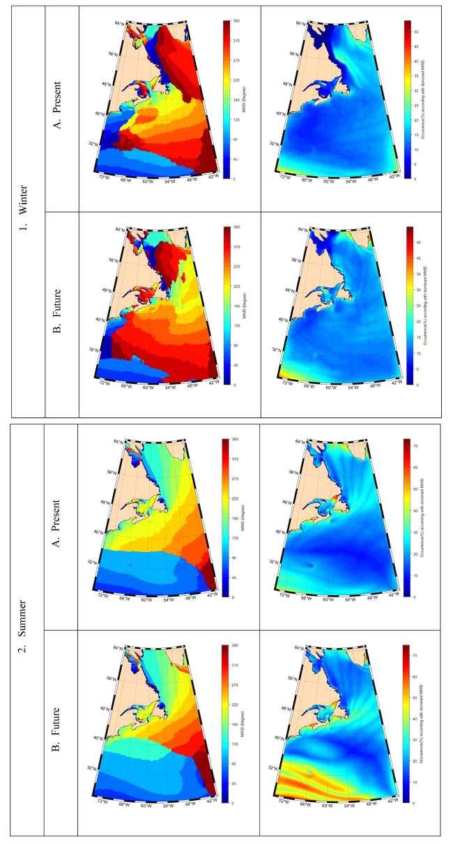
Fig. 3. Dominant mean wave directions in the study area for (1.) wintertime, and (2.) summertime, (A) present and (B) future climate, and (i) dominant MWD, (ii) occurrence (%). |
➢Mean wave direction during winter season
In Fig. 3 panels 1Ai, and ii, dominant mean wave directions for the present winter climate and corresponding occurrence percentages are depicted. The results show that between 5 to 30 percent of waves come from the N-E (0-90°) direction (blue colours), in the areas to the north of Newfoundland and Labrador, south of Gulf of St. Lawrence Sea, southeast of Greenland, as well as southwest of the study area. Some small areas to the east and north of Nova Scotia experience waves in the E-S direction (90-180°) (green colours) with occurrence between 10 to 20 percent. Waves in the direction of S-W (180-270°) mostly come from the central part of the study area (yellow colours) with occurrence between 10 to 20 percent. Waves in a large area of the southeast and northeast of the study area, some parts of Hudson strait, and Gulf of St Lawrence come from W-N (270-360°) directions (red colours) with occurrence between 20 to 35 percent.
For the climate change scenario, in spite of some changes in dominant wave direction patterns in specific areas, the dominant wave direction patterns are preserved, as shown in Fig. 3 panels 1Bi and ii. The results show that most of the waves come from N-E (0-90°) direction (blue colours) with occurrences that vary between 5 to 48 percent, specifically in areas north of Newfoundland and Labrador, coastal areas off southeast of Greenland, and the southwest part of the study area. Some small areas to the east and north of Nova Scotia, the northeast part of the study domain, and Davis Strait are also expected to experience waves in E-S directions (90-180°) (green colours) with occurrences between 10 to 30 percent. Waves in the S-W direction (180-270°) can be mostly seen in the central part and northeast part of the study area (yellow colours) with occurrences between 10 to 15 percent. Moreover, waves in large parts of the south and north regions of the study area, some parts of Hudson strait, Gulf of St Lawrence and Labrador Sea, come from the W-N (270-360°) direction (red colours) with occurrences between 10 to 35 percent.
➢Mean wave direction during summer season
In Fig. 3 panels 2Ai, and ii, the dominant mean wave directions in the study area for the present summer climate are displayed. The results show that most of the waves come from the N-E (0-90°) direction (blue colours) with varying occurrences between 15 to 40 percent, for areas off the north coast of Newfoundland and Labrador, the southern part of the study area, and Ungava Bay. In coastal areas of Nova Scotia, northwest part of Labrador Sea, and Hudson Strait, between 20 to 60 percent of waves come from the E-S (90-180°) direction (green colours). Waves in the S-W direction (180-270°) mostly come from the central part of the study area (yellow colours). About 10 to 20 percent of waves in the southwest part of the domain come from the W-N (270-360°) direction (red colours).
For the future climate, as shown in Fig. 3 panels 2Bi, and ii, although similar patterns to the present climate are evident, waves in N-E direction (0-90°) are present, extending to the central part of the study area and their occurrences are increased by 70 percent. Waves in the E-S direction (90-180°) can be seen in the northwest part of the Labrador Sea, off the east and south coasts of Nova scotia; the occurrences are expected to change between 15 to 45 percent. In the S-W direction (180-270°), we see no significant change in the wave patterns, compared to the present climate, whereas waves in the W-N direction (270-360°) are expected to extend to central parts of the domain, and their occurrences to change, by between 15 to 30 percent.
3.2.2. Significant wave heights
In order to determine the maximum ranges of significant wave heights and corresponding occurrence (%), during winter and summer seasons for the present and future climates, the dominant occurrences of maximum significant wave heights in each computational element were estimated and presented in Fig. 4. In each element, the occurrences of Hs in 17 sub-ranges were calculated (Hs: <1, 1-2, 2-3, 3-4, 4-5, 5-6, 6-7, 7-8, 8-9, 9-10, 10-11, 11-12, 12-13, 13-14, 14-15, 15-16, and >16), and the maximums for Hs in these sub-ranges were extracted during the modeling periods. Thereafter, the corresponding incidences of maximums in the sub-ranges of Hs in each element were computed. As an example, we take one element in the northern part of the Bay of Fundy. The maximum Hs during present wintertime is 2-3 m, and the corresponding occurrence is 0.1% which is reasonable and unsurprisingly small. There is a subtle difference between this method and other standard methods for extracting maximum Hs and corresponding occurrence (%). Specifically, in this method the maximum range of Hs, including all values in a defined range, are calculated and then the corresponding occurrence is extracted. By comparison, in more simple standard methods, the maximum value of Hs during the modeling period is selected and its occurrence is extracted. Selecting the maximum range instead of the maximum value can bring about a much better understanding, in comparison with other methods. Moreover, this method helps to promote insight regarding the occurrences of maximum events and identification of different regimes in the study area. For example, at a specific location during the 39-year time interval, if the maximum Hs is 4.887 m and its occurrence is 0.003%, then based on our calculation the maximum range of Hs is 4-5 m and the corresponding occurrence is 1.5% because we take all data in the range 4-5 m into account. Accordingly, the maps prepared in this study follow this idea. In the following sections, the maximum Hs values and their corresponding incidence percentages for the present and future climate conditions and winter and summer seasons are studied.
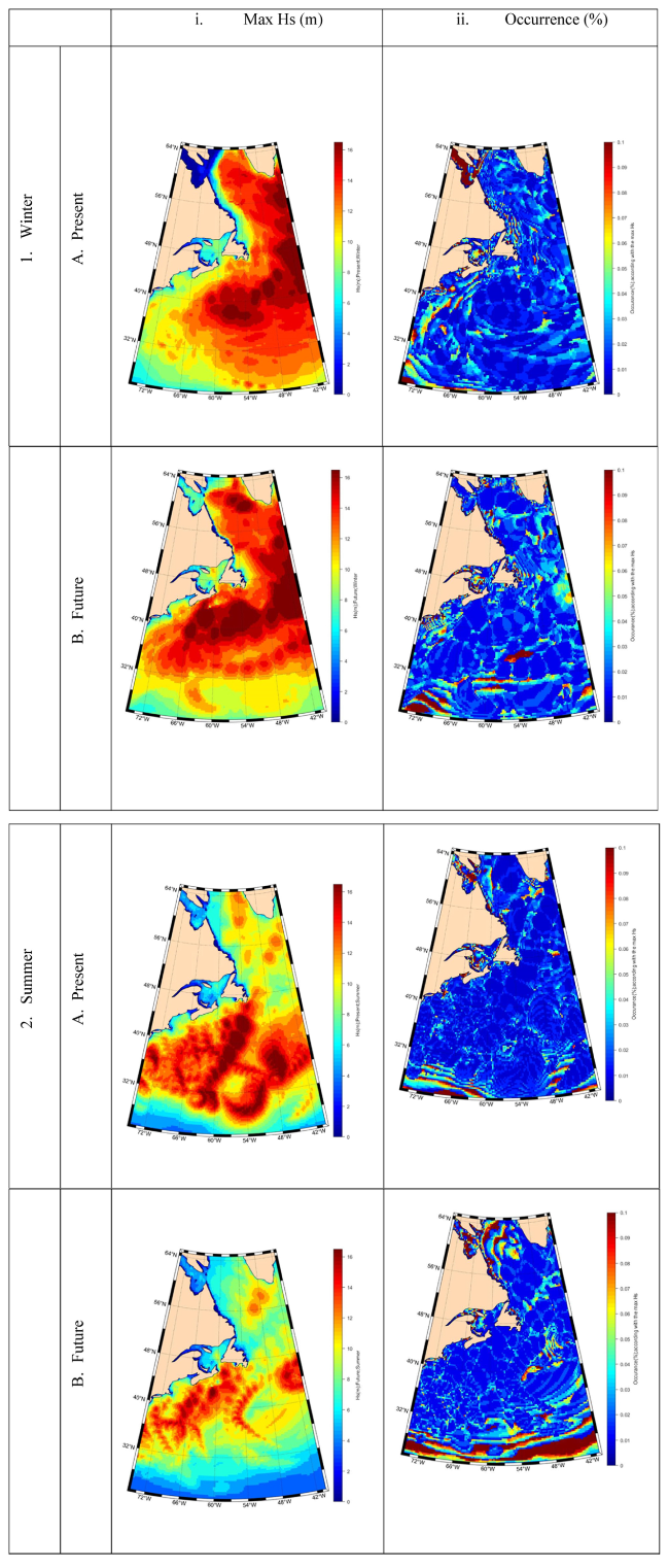
Fig. 4. Present winter season, (i1A) maximum Hs, and (ii1A) occurrence percentage. Future winter (i1B) maximum Hs, (ii1B) occurrence percentage. Present summer season, (i2A) maximum Hs, (ii2A) occurrence percentage. Future summer scenario, (i2B) maximum Hs, (ii2B) occurrence percentage. |
➢Significant wave height during winter seasons
Fig. 4 panel 1Ai shows the maximum values of Hs for the present winter season. Almost all areas beyond the coastal areas are in the range of Hs>10 m, whereas coastal and nearshore areas, like the Gulf of St. Lawrence, experience smaller values. Northern areas like Hudson Strait and Ungava Bay have wave heights in the range of 0 to 1 m because of winter sea ice. The corresponding percentages of incidence for maximum Hs range for the present wintertime climate are depicted in Fig. 4 panel 1Aii. Results show a higher percentage of incidence in the northwest part of the study area because of sea ice during the winter season. By comparing the two panels (1Ai and 1Aii), we infer that although areas with higher values of Hs (>10 m) cover most of the open ocean areas, the percentage occurrence map is similar over most of the study area
Similar analyses was carried out for the future winter scenario in Fig. 4 panels 1Bi and 1Bii. Results imply that maximum Hs values are estimated to be greater than 10 m and extend towards the western part of the study area, closer to coastal areas, compared to the present climate. A notable change is that higher values of Hs are estimated to occur in the northwest part of the study area, with relatively high waves extending even into Hudson Strait and Ungava Bay, reflecting an expected reduction in sea ice in the future scenario, even during winter season. In this situation, the occurrence percentage exhibits a similar pattern in the future climate as for the present climate, modulated by a slight movement of the area with the highest percentage of incidence towards the central part of the study area. Meanwhile, in Hudson Strait and Ungava Bay, although the maximum Hs range tends to increase, the incidence percentage appears to notably decrease.
➢Significant wave height during summer seasons
Fig. 4 panel 2Ai shows the maximum values of Hs for summer seasons in the present climate. Most areas with range Hs>10 m are far from the coast, whereas the percentage of occurrences in areas in this range of Hs are similar and in the range of smaller than 0.01%. Smaller values for maximum Hs are also expected in other areas, including almost all of the coastal areas, the northern part of the Gulf of St. Lawrence, Davis and Hudson Straits, Ungava Bay. On the other hand, areas such as the southern and northwest parts of the study area, Bay of Fundy, and southern part of the Gulf of St. Lawrence experience a higher percentage of occurrences. For the present winter climate, the percentage of incidence values corresponding to maximum Hs are shown in Fig. 4 panel 2Aii.
A similar analysis is carried out in Fig. 4 panels 2Ai and 2Aii, for the future summer scenario, showing maximum Hs values that exceed 10 m in many areas except the extreme northwest, west, and southwest parts of the domain, adjacent to coastal areas. Despite significant increases in areas with Hs>10 m, the maximum Hs in the most of these areas will decrease compared the present climate. In other words, maximum wave heights in areas with smaller significant wave heights are bound to increase, whereas maximum Hs in areas with higher Hs tend to decrease for the future climate change scenario. In addition, in Hudson Strait, Hs values appear to decrease during summer seasons; in other coastal areas Hs is expected to increase. The occurrence percentage for this condition, also represents a considerable increase especially in the northwest and southern parts of the study domain.
3.2.3. Mean wave period parameter
For analysis of mean wave period (T0), and corresponding occurrence (%) for winter and summer of present and future climate scenarios, values for each element are calculated and displayed in Fig. 5. Thus, in each element, the occurrences of T0 in different ranges (T0: <4, 4-6, 6-8, 8-10, 10-12, 12-14, and >14 s) are calculated; the maximum T0 ranges during the modeling period are extracted and the corresponding incidence percentages in each element are computed. As an example, consider one element in the center of the Gulf of St. Lawrence. The maximum T0 during the modeling period for the present winter climate is in the range of 10-12 s, and the corresponding occurrence with this range of T0 is 0.011%. The methodology to extract T0 maps is similar to that for Hs maps. Results for maximum T0 values and corresponding incidence percentages for present and future climates, and winter and summer seasons, are presented.

Fig. 5. Maximum range of mean wave period T0 and corresponding occurrence percentage for: (i1A) T0 the present winter climate, (ii1A) occurrence percentage for present winter climate, (i1B) T0 for future winter scenario, (ii1B) occurrence percentage for future winter scenario, (i2A) T0 for present summer climate, (ii2A) occurrence percentage for present summer climate, (i2B) T0 for the future summer scenario, (ii2B) occurrence percentage for future summer climate. |
➢Mean Wave Period during winter season
According to Fig. 5 panel 1Aii, maximum T0 ranges in areas including Hudson Strait and Ungava Bay are between 4-6 s and the incidence percentages are higher than 0.09%. By comparison, in the southeast part of the study domain, these values are in the range 11-12 s and the incidence percentages are between 0.01 to 0.04%, and in the west part of the study area, we expect 13-14 s and the incidence percentages are higher than 0.09%. For the future climate in Fig. 5 panel 1Bi, an increasing trend can be easily identified in most areas, from deep water to adjacent coastal areas. In Hudson Strait, the maximum wave period ranges have an increasing trend that may be due to climate change impacts on non-frozen northern waters during the winter season. The incidence of maximum wave period ranges for the future winter season is depicted in Fig. 5 panel 1Bii. Results show that the percentage of incidence for these maximum values will decrease in the entire study area, due to climate change.
➢Mean Wave Period during summer season
For the present summer climate, Fig. 5 panel 2Ai shows the maximum T0 values. Results imply that some scattered areas in the east, southeast, west and center, including Davis Strait, experience wave periods exceeding 14 s. By comparison, other areas including Hudson Strait, Ungava Bay, Gulf of St. Lawrence, and southern Labrador Sea suggest values of T0 in the range of 5-12 s. A similar analysis is carried out for the future summer scenario in Fig. 5 panels 2Bi and 2Bii. Unlike the future winter scenario, the maximum T0 values are considerably reduced and areas with T0>14 s can be recognized only in the west center of the study domain. The percentage of occurrence in the study domain varies from 0 to 0.1%. Some scattered areas in northwest Labrador Sea, central Gulf of St. Lawrence, southwest and southeast areas in the study area show the highest values of occurrence percentage.
3.3. Training geosom and visualizations
In this paper, we apply the GeoSOM algorithm in SPAWNN, a toolkit for SPatial Analysis with Self Organizing Neural Networks, which developed as a standalone, independent, open-source application software under the GNU General Public License (GPL) [73]. GeoSOM is used to discover the outliers. This is a key step because the data distribution can be distorted by outliers, thereby affecting the follow-on analysis.
To project the NG output layer, the neuron numbers were determined as 234, based on the methodology we applied to identify the optimal number of clusters. We follow the approach of Martinetz et al. (1993), regarding linear and power methods for the neighborhood and adaptation options. Thus, the power method was considered and the initial and final values for neighborhood are taken as λi=25, λf=0.01. For the adaptation method, these values are εi=0.5, εf=0.005. By trial and error, we find that the training cycles are restricted to tmax=1,000,000.
To confirm these estimated values, we conducted primary tests and associated analysis that revealed a fair agreement between the computational effort needed for training the networks. To conduct spatial clustering of the wave regime parameters (Hs, T0, and MWD), a 34 × 161 × 141 matrix was taken into account to extract normalized wave parameter data for the present climate from 1979 to 2017 (39 years). Here, 34 is the number of sectors, 161 and 141 are the number of elements in X and Y directions, respectively, based on numerical wave model outputs. The raw data was extracted from the outputs from the WWIII wave model. Fig. 6(i) displays the projected geographical map and clusters in the study area and Fig. 6(ii) shows the neighbor weight distances that originate from the two-dimensional NG output layers. As seen in Fig. 4, there are 234 clusters that are discerned in the study area; each cluster includes 34 parameters composed of Hs (11 groups), T0 (7 groups), and MWD (16 groups) that have maximum similarity and homogeneity with each other. In other words, each cluster includes the waves which have essentially identical percentages of defined ranges for Hs, MWD, and T0.

Fig. 6. (i) projected clusters in the study domain, and the corresponding color for each cluster number. (ii) 2-dimensional Geo-NG components of wave parameter data. |
3.4. Extreme value analysis (EVA)
In hydrodynamic modeling of the ocean, for applications like the design of marine structures etc., one of the fundamental steps is an extreme value analysis, for example for studies of coastal erosion, risk analysis for inundation in coastal areas, and related concerns. In order to determine the extreme values for wave parameters, two parameters are adopted, Hs and T0. Based on our NG clustering analysis, 234 representative points including 6-hourly time series for the present climate (1979 to 2017) and future climate scenario (2060 to 2098), for winters and summers were selected. Thus, an extremal analysis is conducted for Hs and T0 time series at the centroid points, for the present and future winter and summer seasons, for 5 and 100-year return periods.
➢Extremal analysis of significant wave heights
Extreme values for Hs for winter in the present climate for the 5-year return period are given in Fig. 7 panel 1Ai. Values are between 0 m and 1 m for the northwest part of the domain, in Hudson Strait and Ungava Sea, and continue in this range for much of the northeast coastal area, including the Gulf of St. Lawrence, coastal areas of Newfoundland and Labrador, and waters off Nova Scotia and Bay of Fundy. Deeper offshore waters have higher extreme values for Hs, up to 15 m in the eastern part of the study domain, reflecting the longer fetch along the dominant North Atlantic storm track, particularly between 40- and 60-degrees north latitude.
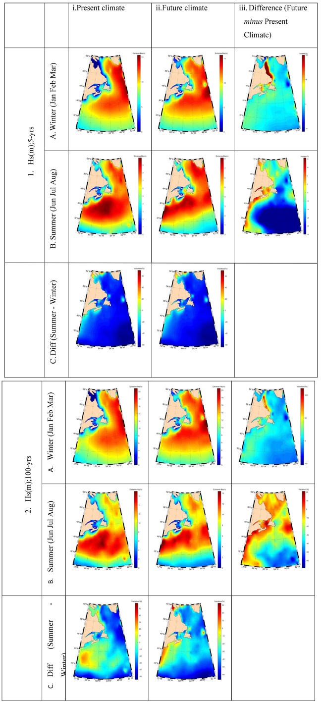
Fig. 7. Extreme Hs values for (i.) present climate, (ii.) future climate scenario, (iii.) difference of future minus present climate (%). The 5-year return period is shown in (1.), and the 100-year return period in (2.). Winter season is A, summer season is B, and the difference of summer minus winter season (%) is C. |
Estimates for extreme values for Hs for the future winter climate scenario, are given in Fig. 7 panel 1Aii. Although the results are similar to those of the present climate, there also are differences, as shown in Fig. 7 panel 1Aiii. For example, extreme values of Hs are estimated to clearly increase in most open ocean areas, by up to about 20%. For particular areas, such as waters off the Labrador coast, the change in extreme Hs values can be as much as 100% due to reductions in sea ice, and to a lesser extent, changes in North Atlantic storms. Other areas experiencing notable change in extreme values for Hs are the Gulf of St. Lawrence, and northern waters off Newfoundland and southern Baffin Bay.
For the present summer climate, most coastal and nearshore areas in waters off North America experience extremes in Hs of up to about 3 m. This is displayed in Fig. 7 panel 1Bi. Higher values tend to occur in deeper waters in open ocean areas reaching up to about 10 m in central and eastern regions of the study domain. This reflects the intensity of the dominant summer hurricane storm tracks in the North Atlantic. By comparison, extremes in Hs for the future summer scenario tend to have lower values for most of the study domain, as shown in Fig. 7 panel 1Bii. The maximum is about 8.0 m. Differences between present and future summer scenario are displayed in Fig. 7 panel 1Biii. Areas where extremes in Hs might be expected to increase, up to about 15% or so, are estimated in areas such as Hudson Strait, the Gulf of St. Lawrence, coastal areas, and southwest areas of the study domain. Most offshore and open ocean areas experience notable reductions in extreme Hs, as much as 30%.
More comparisons are given in Fig. 7 panels 1 Ci and ii to assess the changes of extreme Hs between summer and winter seasons in each climate condition. In the present climate, the results suggest extreme Hs values experience changes between summer and winter that are between 0 to 70% in some coastal areas, particularly in the northeast part of the study domain (e.g., Hudson Strait and Ungava Sea), due to changes in sea ice conditions. Other areas show decreases, ranging from 0 to −60%, with maximum reductions occurring in eastern and southeastern parts of the domain. In the future climate scenario, changes in extreme Hs between summer and winter are also between 0 to 70%, particularly in Hudson and Davis Straits areas, whereas other areas experience reductions, also in the range 0 - 60%, with maximum decreases occurring in southeast parts of the study domain.
For 100-year return period, we show the extreme Hs values and the differences in Hs values for the present climate and the future scenario climate, and for winter and summer seasons in Fig. 7 panel 2. This suggests that the patterns for Hs extreme values, and their changes, are similar to those for the 5-year return period. Unsurprisingly, the values for Hs extremes are larger for the 100-year return period than for the 5-year return period; however, some areas such as Hudson Strait remain unchanged, because of the sea ice regime.
➢Mean wave period extreme values
For present winter conditions, extreme mean wave periods, T0, for a 5-year return period are shown in Fig. 8 panel 1Ai. Relatively low values are estimated for coastal waters off North America with notable maximum low extremes in T0 (less than 2 s which is negligible) suggested for Hudson Strait and Ungava Bay in the northwest, the Gulf of St. Lawrence, waters around the St. Lawrence Estuary, Anticosti Island, Prince Edward Island and Nova Scotia. Extremes for mean T0 in coastal areas are typically in the range between 3.3 to 7.5 s which are still much lower than open ocean areas, e.g., beyond the continental shelf. More distant areas beyond the coast are estimated to have higher values for extremes in T0. The largest values tend to occur in Davis Strait and southwestern areas of the Labrador Sea. These areas are relatively remote from the dominant North Atlantic storm track region.
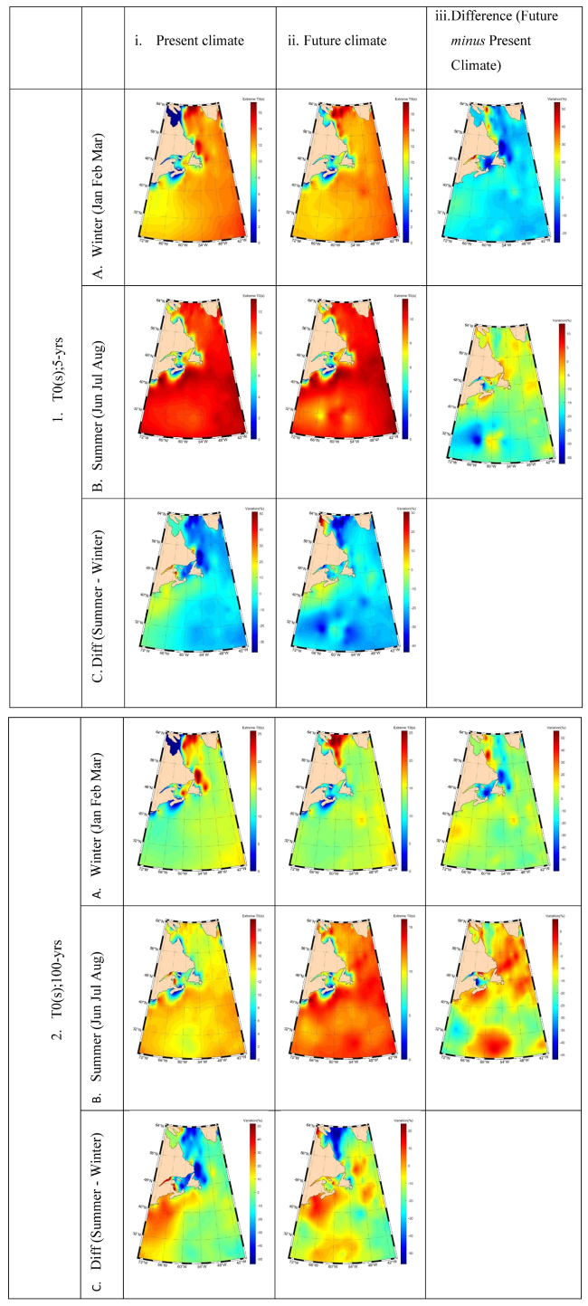
Fig. 8. Extreme T0 values for (i.) present climate, (ii.) future climate, (iii.) difference of future minus present climate (%). The 5-year return period is shown in (1.), and the 100-year return period in (2.). Winter season is A, summer season is B, and the difference of summer minus winter (%) is C. |
For the future winter scenario, extreme mean T0 values are estimated in Fig. 8 panel 1Aii. Although similar patterns are suggested for the future climate as were seen in the present climate in panel 1Ai, there are also many areas that appear to experience change. Notable areas are western parts of southern Baffin Bay and western Labrador Sea, where extremes in T0 are estimated to increase to up to 8 sec. or about 50%, as shown in panel 1Aiii. Similar large changes are also estimated for the St. Lawrence Estuary, perhaps 30%−40%. The dominant mechanism for change is reduced sea ice. Changes in storms tracks are estimated to play a relatively smaller role, as suggested by Wang et al. [72].
For the present summer climate, most nearshore and coastal areas in the western part of the study domain are estimated to experience extreme T0 values in the range between 3.0 to 7.0 s. This is shown in Fig. 8 panel 1Bi. Extremes in T0 become larger in coastal regions that are more distant from the shoreline, as well as open ocean regions. Extremes in mean T0 tend to be in the range between 10 to 13 s over a large part of the southwest area of the study domain. By comparison, for the future summer scenario, extremes in T0 have similar patterns. Comparing future minus present, differences in extremes in T0 are in the range up to about +10 to −35%, as indicated in Fig. 8 panel 1Biii.
More comparisons were done to assess changes of extreme T0 between summer and winter seasons in Fig. 8 panels 1 Ci and 1Cii. For the present climate, the difference of summer minus winter suggest increases of between 0 to 50% in the southeastern parts of the study domain, whereas other areas experience decreases of 0 to 40% and maximum reductions in Davis Strait and the Labrador Sea. Correspondingly, in the future climate, results suggest decreases by 0 to 44% in northern and southern parts of the study domain, with maximum reductions in Davis Strait. Some coastal areas can experience increasing trends; as an example, maximum increases in T0 are estimated up to 30% in Hudson Strait.
Extreme T0 values and differences in T0 extremes for the present climate and future climate scenario, for winter and summer seasons, are presented for the 100-year return period in Fig. 8 panel 2. These patterns and their expected changes are similar to those suggested for the 5-year return period. As with Hs, it is not surprising that estimates for extremes in T0 are increased for the 100-year return period, compared to the 5-year period. This increase is up to about 9 s in the northwest region of the domain, around Davis Strait, for the future winter climate, reflecting the expected reductions in sea ice in a warming climate.
4. Conclusions and discussion
The objective of this study was to construct a comprehensive assessment of wave regime and extreme values, for the present climate and future climate scenario, for winter and summer seasons in the Northwest Atlantic. In this regard, wave parameters, Hs, T0 and mean wave direction, MWD, for two 39-year periods were considered; the present climate represented by 1979-2017, and the future climate represented by 2060-2098. These data sets were simulated by WW3 model following IPCC climate scenario RCP8.5.
Using these data sets, wave characteristics in the entire study area were studied and areas with different ranges of Hs, T0 and MWD were extracted. A comprehensive understanding of the wave regime in each part of the study area was obtained, for winter and summer seasons and for current and future climatic conditions. In order to assess the extreme wave parameters in the entire study area, we used the GeoSOM clustering method, and applied the Neural Gas technique. Thus, for centroid points of 234 clusters, time series of Hs, T0, and MWD were extracted for four data sets; namely, present climate for winter and summer seasons, and future climate scenario also for winter and summer seasons. Extreme values for 5-year and 100-year return periods were estimated using three stochastic models; Gumbel, Exponential and Weibull distribution functions.
Unsurprisingly, the wave regimes for winter and summer seasons are completely different. Although wave patterns for the present climate and future climate scenario are somewhat similar, there are also scattered areas where notable changes occur due to the impacts of climate change. A dominant factor is sea ice. In the future climate scenario, areas of the Gulf of St. Lawrence, Labrador Shelf, southern Baffin Bay and Hudson are expected to experience notable reductions in sea ice and more open water. In general, low values of Hs correlate with low values of T0; and similarly for respective high values of these variables. But it is not possible to establish reliable correlations of either variable to MWD, in general over the study domain. Following the dominant North Atlantic storm track region, Hs tends to increase towards the northeastern region of the study domain.
Our results are consistent with earlier studies, for example Wang and Swail [74]. The impact of climate change tends to increase extreme values of Hs in northwestern coastal areas in winter, and to decrease Hs in central parts of the study domain during summer. These trends reflect the two main factors due to climate change, the modulation of the dominant North Atlantic storm tracks, and reduction in sea ice.
Data Availability Statement
Marine winds to drive WW3 are provided by a regional climate model simulation as described by Zhang et al. [75], driven HadGEM2-ES global climate model following IPCC AR5 climate change scenario rcp8.5. The latter data are available on https://esgf-index1.ceda.ac.uk/search/cmip5-ceda/
Declaration of Competing Interest
The authors declare that they have no known competing financial interests or personal relationships that could have appeared to influence the work reported in this paper.
Acknowledgments
We were supported by Canada's Competitive Science Research Fund (CSRF) Program, Ocean Frontier Institute and Marine Environmental Observation, Prediction and Response Network in this study.
