
Abbreviations and notations
ϵR: relative error (-)
ρ: material density (kg.m-3)
C: speed of sound in medium (m.s-1)
B: plate breadth (m)
Bs: mesh base size (m)
Cf: force coefficient (-)
Cp: pressure coefficient (-)
D: thickness of air cushion (m)
CFD: computational fluid dynamics
CFL: courant number (-)
DOF: degrees of freedom
F: impact force (N)
K: kinetic length of fluid (m)
Km: velocity reduction coefficient (-)
M: plate mass (kg)
MA: hydrodynamic added mass (kg)
p: pressure (Pa)
P1, P2, P5: recorded pressure points (Pa)
t: CFD solution time (s)
T0: duration of impact (s)
U: velocity of water (m/s)
v: impact velocity (m/s)
VOF: volume of fluid
%ap: percentage of pocket area to plate area ratio
%tp: percentage of pocket depth to plate thickness
%volp: percentage of pocket volume to plate volume
ΔL×ΔW×Δt: dimensions of air pocket (mm)
1. Background
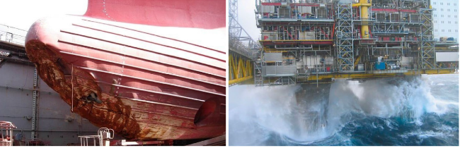
The effects of impact pressures resulting from a solid's interaction with a liquid's free surface have been a topic of investigation by numerous methods of analysis for the greater part of the last century, ongoing to the present day [5,18,20,30,37]. As shown in Fig. 1, the significance of accurate prediction of slamming force and pressures lies in engineering applications for coastal and offshore structures, fluid sloshing effects in tanks, the marine industry, and amphibious aircraft. In an attempt to quantify the anticipated magnitudes of fluid impact loading on fixed and floating structures in maritime environments, many offshore industry codes of practice provide inexplicit solutions for the prediction of slamming pressures. In practice, both API-RP-2A and ISO 19902 acknowledge that the water-free surface's shape, entrained air's compressibility, and the air-water presence during wave slamming may influence forces. Nevertheless, the slamming force in the current design practice is simply calculated by a variant of the drag equation [4,12,16]. Recently, the American Bureau of Shipping (ABS) classification society has developed guidance notes on wave impact analysis which provide a similar perspective to the API and ISO approaches such that the wave impact pressure coefficient is not specified and must be determined by the user [3]. DNV-RP-C205 recommended practice expands on a similar method through the inclusion of a slamming force coefficient dependent on submergence, and a geometry-specific slamming pressure coefficient; the latter is supplied with a condition that the approach should not be employed for the prediction of extreme local pressure values [12]. This acknowledgement of the complicated nature of local processes which may occur during wave slamming events without the offer of full remediation constitutes the necessity for enquiry into the behaviour of these phenomena.
Recent advancements in numerical analysis in fluid dynamics, heat and mass transfer using high-fidelity methods such as Computational Fluid Dynamics (CFD), Smoothed Particle Hydrodynamics (SPH) and Lattice Boltzmann Method (LBM) have solved complex fluid-structure interaction problems including the prediction of slamming forces and localised pressures on structures with air entrapped in pockets that are formed by the shape of the fluid's free surface during impact and/or the geometry of the solid surface itself [2,6,18,38]. For instance, [6] conducted a numerical study into hurricane wave events on concrete bridge girders concluded using Reynolds-Averaged Navier-Stokes (RANS) and compressible Euler equation CFD solvers and found that viscous effects of fluid are negligible in these types of scenarios. His experimentally validated model experienced a reduction in hydrodynamic forces by the implementation of the bridge deck or diaphragm outlets to vent air entrained within the structure. The role of entrapped air on the underside of coastal bridge decks was scrutinised in a similar analysis by the simulation of non-linear shallow-water waves. These were modelled to collide with a structure in a numerical wave tank employing a volume of fluid (VOF) based approach. The authors concluded that the air compressibility in the two-phase model had a slight cushioning effect [31].
A recent study conducted by [2] reaffirmed these findings in the scenario of wave slamming on the underside of a fixed offshore platform. The deck underside experienced a significant reduction in slamming pressure magnitude (∼22%) when the air phase was modelled in CFD as compressible. Another key finding of this investigation was the significance of the air phase fraction during peak pressure events; a high air proportion was present in all simulated cases. Other studies have proven that the reduced inertia and high compressibility of a volume of air allow for rapid accelerations of fluid mass, consequentially amplifying pressure surges. Research into this phenomenon has concluded the existence of a critical volume, resulting in the greatest magnitude of pressure impulse [23]. Kim et al. [18] developed a CFD model of wave slamming events on a spar-type vertical column and identified the importance of the air volume fraction in these phenomena. The author's proved compressibility's influence on the speed of sound in water, cwater and subsequent pressure results; testing of a lower cwater value yielded lower pressure magnitudes.
Lately, slamming load prediction by drop tests has attracted many researchers both experimentally and numerically. Physical drop tests are useful for assessing pressure sensors and providing values for the validation of CFD tools, in particular incompressible flow conditions [11]. For example, Zhang et al. [40] modelled perforated plates with different aspect ratios and discovered their slamming coefficients numerically using the VOF and URANS equations. They realised that the compressibility of air influenced the slamming force and reduced it considerably on the flat plate water entry. Nair and Bhattacharyya [26] conducted a CFD study utilising a VOF scheme implemented in FLOW3D software to capture the free surface accoiated with the water impact and subsequent entry of three rigid axisymmetric bodies, a sphere and two cones. They concluded that while the penetration depth, vertical velocity and vertical acceleration time histories were reproduced well by CFD in comparison with experimental results, the peak pressure on impact required a much finer mesh and appropriate choice of the time step. Furthermore, Mai et al. [22] conducted an experimental study by dropping a rigid flat plate in a free-falling scenario onto aerated and non-aerated water conditions, and the pressure distribution on the bottom of the plate was recorded. As a result, it was deduced that aeration decreases the impact load not only due to the air presence but also water surface distortion. In addition, Truong et al. [35] conducted a numerical investigation into the slamming on a flat-stiffened plate considering the fluid-structure interactions and stated that the air cushioning effects should be considered during very small deadrise impacts because of resulting different responses and due to longer impact duration. Moreover, Swidan et al. [32,33] predicted the slamming loads on wedge-shaped catamaran hulls utilising CFD and experimental investigations. They concluded a relationship between the body velocity and slamming force. On the other hand, CFD results showed a better agreement to the experiment than 2D SPH which is also supported by the findings of Sasson et al. [29].
Notably, it was observed during such model testing and numerical simulations of drop tests that air entrapment and the formation of air pockets between the impacting object and the water surface become inevitable. Chung et al. [10] experimentally ascertained that air pockets at low angles of incidence tend to reduce the impact pressure and when the angle of incidence increases, a jet is generated. Kang [17] conducted an experimental investigation into shallow-water impacts, and Oh et al. [27] analysed the generation process of air pockets during a flat impact of a box-type model. Elhimer et al. [13] also found a reduction of the impact load when a cone enters a gas-liquid mixture due to the increase in the air volume fraction. However, as concluded in these studies the quantitative assessment of the effect of generated air pockets remains challenging.
It can be noted that there is a lack of research into the role of air entrapment associated with slamming events in particular water impact loads on offshore structures such as jacket structures, jack-ups and semisubmersibles which have different hull forms from ship structures. The deck underside of such structures may attract air to be entrapped during the water impact loading process. Furthermore, the current design practices for offshore structures do not consider the effect of air phase or its compressibility on the magnitude, scaling and distribution of slamming forces and pressures. Such research efforts should include systematic investigations into the quantification of the air content, air/water compressibility and the shape of air pockets. As recommended by Dias and Ghidaglia [11] in their review on the recent progress on the evaluation of impact/slamming pressures, CFD analyses could be useful to identify the type and nature of impacts.
The study detailed in this paper aims at developing a numerical simulation of a flat plate still water entry process to isolate a solid-meets-liquid impact event such that the effect of air entrapment can be quantified. With a functionally verified and validated CFD model the various theoretical methods of shock pressure prediction may be evaluated. Subsequently, physical parameters such as the inclusion of a void (pocket) on the plate's impact surface to encourage the entrapment of air are incorporated into the model and resultant responses observed. Considerations will be given to the compressibility of both air and water phases, and the phase volume fraction during simulation attempts. Monitoring of the many loading impact processes that occur in a relatively small timeframe will provide a thorough understanding of the phenomena associated with slam events.
The remaining sections of this paper are set out as follows: Section 2 reviews the theoretical studies of water impact problems. Section 3 describes the CFD approach and numerical simulation setup for flat plate and air pocket models for which the commercial CFD STAR-CCM+ code was used in this analysis with simulations executed on the University of Tasmania (UTAS) Kunanyi cluster. Section 4 discusses the obtained results of numerical tests for different conditions. Section 5 concludes the main findings of this study.
2. Review of theoretical studies
Theoretical analysis of solid-liquid impact phenomena has been a focal point of research pioneered by Von Karman [37] on his studies of seaplane float impacts during landing. This simplified momentum theory approach of a unit-length two-dimensional wedge-shaped solid striking a flat surface of incompressible, inviscid fluid laid the foundation for drop-test style research on slamming pressures of perpetually increasing intricacy. Although the primary finding of this study was an experimentally validated formula for peak localised pressure (pmax) occurring at the centre point of the wedge, the asymptotic nature of the equation resulted in pmax→∞ as the float deadrise angle, α→∞ due to the incompressible characteristic of the fluid. Subsequent investigation on a flat-bottom float identified that the propagation of shock pressure on the solid occurs at the fluid's speed of sound, cwater. The resulting equation given in Eq. (1) is
$p_{\max }=\frac{\rho v^{2}}{2}\left(\frac{2 c_{\text {water }}}{v}\right)=\rho v c_{\text {water }}$
where ρ is fluid density, was concluded to overestimate experimental pressures due to elastic deformation of the float's surface upon impact. A US Navy report by Chuang [9] on the effects of slamming highlighted this overestimation, accrediting it to a compressible layer of air trapped between the impacting body and the water free surface. The cushioning effect from this layer of air was observed to impose a greater rise time of the impact pressure pulse, some of which would be forced into the adjacent layer of water to create an inhomogeneous mixture of air and water, greatly reducing both ρ and c. Consequentially, Chuang's formula (Eq. (2)) derived through theoretical reasoning and experimental observation incorporated cair for the calculation of impact pressures, predicted in imperial units as
$p_{\max }=\frac{\rho c_{\text {air }} v}{32 \times 144}\left(\frac{1.4+\pi^{2}}{e^{-1.4}+1}\right) \approx 4.5 v$
in psi (v in ft/s) for a 116 kg plate, [L×B] = [510 × 675] mm. Chuang hypothesised plate mass (M) and hydrodynamic added mass (MA) to be contributing factors in the generation of slamming shock pressure. As seen in Eq. (3), Okada and Sumi [28] built on Chuang's findings, implementing these parameters into theoretical formulae through the integration of a MA-dependant velocity reduction coefficient (Km) to their pmax equation,
$p_{\max }=\frac{M_{A} K_{m} v}{B T_{0}}$
Where Km=MA(M+MA)−1 and 1/T0=0.144×103(v/B)0.673 (T0 is the empirically derived duration of impact). MA is calculated on a unit length basis as ρπB2/8. This equation was proven to agree with experimental results for B = [200-600] mm plates up to v= 3.25 m/s for a range of masses between 70 and 135 kg.
The first attempt of modelling compressed air entrapped between liquid and solid impact surface was performed by Bagnold [5] to study ocean wave behaviour impacting a vertical wall in a controlled environment. Representing the wave impact event analytically as a 1D water piston in an adiabatic process, Bagnold's assessment of the impulsive force created by the compressed layer of air highlighted the existence of a parameter deemed the kinetic mass of the breaking fluid (ρAK). The piston volume was calculated as an area equivalent to the cross-sectional area (A) of a body travelling through the fluid of length K in the direction of motion. Using wave pressure data from oscillograms and momentum theory, the length K from each impact event was back-calculated using Eq. (4) as
$K=\frac{\int^{p} d t}{\rho U}$
where U is the velocity of advancing water, K was empirically discovered to coincide with one-fifth of wave amplitude. Employing D as the thickness of the air cushion between wave and solid surface, the pressure rise during impact was concluded to be:
$\frac{p_{\max }}{p_{0}}=1+2.7 \frac{\rho U^{2} K}{p_{0} D}$
within ±10% of full-scale experimental values for results between 2 and 10 atmospheres of pressure (p0 denotes atmospheric pressure). Developing a similar methodology of wave-impact research, Mitsuyasu [25] validated Bagnold's analytical solution experimentally, expanding the analytical model for a larger momentum of water mass through an assumption of finite compression of the entrapped air pocket as
$\frac{p_{\max }}{p_{0}}=1 \pm 1.18 \sqrt{\frac{\rho U^{2} K}{p_{0} D}}+12 \frac{\rho U^{2} K}{p_{0} D}$
The formula included ± to account for the minimum value of oscillating pressure observed post-impact. Mitsuyasu acknowledged the complexity of the actual water-air-solid junction, found to generate numerous simultaneous mechanisms occurring locally at differing regions of the impact zone. It was thus concluded that pressure maxima are caused by compression of the entrapped air cushion.
As was highlighted above, deck impact loads (also known as wave-in-deck loads) are one of the most critical loading events that affect the structural design of offshore structures. However, due to physical complexities generated by the presence of air pockets on the underside of top-deck structures, i.e., air entrapped between structural members during the wave impact, accurately predicting the magnitude and distribution of the wave impact loads is still a major technical challenge. The principles of Bagnold and Mitsuyasu can be adapted for the offshore engineering practice by developing an equivalent simplified drop test on the basis of wave paramteres, air gap and deck geometry. Fig. 2(a) depicts an orthogonally stiffened deck which is one of the most common methods to increase the strength of a deck plate of an offshore platfrom in order to withstand various loadings including wave impacts. The void spaces created using these longitudinal and transversal structural beams will form air pockets during wave slamming, shown in Fig. 2(b). In offshore practice, such wave slamming loading process can be replaced by a simple drop test. As previously discussed, theoretical studies show that the resultant force and impact pressure affected by forming of air pockets can be related to the depth of the pocket (D), size of the pocket (l = a) and the vertical velocity of the wave (w), which will be fully discussed in the next section.
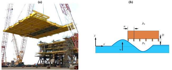
Fig. 2. (a) An orthogonally stiffened deck of an offshore platform and (b) schematic profile view of wave impact and air entrapment for an offshore deck model (not to scale). |
3. CFD investigation
Numerical modelling has recently experienced rapid development and in conjunction with the today's available computer power, CFD tools are used for numerous applications. Various commercial codes, such as STAR- CCM+, ANSYS FLUENT and ANSYS CFX, are available for modelling and solving complex problems such as water entry impact events. The commercial CFD code STAR-CCM+ was used in this analysis with simulations executed on the University of Tasmania (UTAS) Kunanyi cluster. Based on isothermal and laminar flow assumptions, a system of partial differential equations governing the conservation of mass and momentum of a fluid was solved numerically using finite volume method [36].
In addition, the free surface equation and its motion were solved and captured using the VOF model. The VOF model implemented in the solver was then used to determine the relative volume fraction of water and air phases in each computational cell. Physical properties, such as density and dynamic viscosity, were calculated as weighted averages based on this fraction. The VOF model solved the continuity equation for the secondary phase (herein water) to capture the interface between the two phases. The model adopted the homogeneous multiphase theory, which assumes that the velocities of the phases were equal. This required that only a single momentum equation was solved throughout the domain and the resulting velocity field was then shared by the water and air phases [7]. The VOF model also solved volume-fraction equations. To solve these equations numerically, the computational domain was divided into finite control volumes described in the mesh generation section below.
The software discretises the spatial domain into finite volumes (cells), using an unsteady RANS solver to compute unknowns. In turbulent flows, field properties become random functions of space and time. To resolve this, the velocity and pressure fields can be expressed as the sum of mean and fluctuating parts. Substituting these mean and fluctuating terms into the incompressible form of Navier-Stokes equations effectively yields the RANS equations. In this study, the RANS equations were incorporated in one simulation to study the effect of turbulence flow on the loading impact process through the application of the SST k-ω turbulence model which resolves both near field and far field viscous flow [19,24]. For more info about how these equations are implemented in the solver, please refer to the User Guide of the software tool [7].
An implicit unsteady solver is employed with a second-order temporal discretisation using five inner iterations per time step. Six degrees of freedom (DOF) dynamic fluid-body-interaction motion is assigned to the plate; all DOFs but motion in the z-direction (vertical) are constrained. Plate material is assumed rigid and is modelled as such. Solver default atmospheric pressure and material physical properties such as speed of sound, density and viscosity are employed. Where a simulation is run with a compressible air or water phase, user-defined field functions given by Eqs. (7) and (8), were created for instantaneous material density as [1]:
$\rho_{i}=\rho_{i}^{\prime}+\frac{p}{c_{i}^{2}}$
and subsequently its pressure derivative as
$\frac{d \rho_{i}}{d p}=\frac{1}{c_{i}^{2}}$
where ρ and c are the phase's density and speed of sound, respectively (331 m/s and 1450 m/s in air and water, respectively), ρi′ is the reference (incompressible) density of air and water phases (1.18 kg/m3 and 1000 kg/m3 for air and water, respectively), and p is pressure. At every time step, p value is obtained for each node throughout the numerical domain by solving the Poisson equation.
The following solution parameters were found to be important to achieve satisfactory results. These settings were selected as a reasonable compromise between accuracy and computational time. The second-order discretisation of unsteady terms in momentum equations and the High-Resolution Interface Capturing (HRIC) scheme for the solution of the volume fraction equations was adopted in all simulations. The pressure-velocity coupling was performed by the SIMPLE (Semi-Implicit Method for Pressure Linked Equations) algorithm. Second order discretisation for convective terms of VOF model was also selected. It was found that a time step dt of 20 - 100 μs and 5 iterations per time step are adequate to maintain optimal HRIC solution. Pure HRIC scheme is used when the local Courant number, also known as Courant-Friedrichs-Lewy (CFL) number as given in Eq. (9), is below the lower limit (0.5), whereas a pure first-order upwind scheme is automatically activated for Courant number higher than the upper limit (1.0). For intermediate limits, both schemes are blended [7]. It should be noted that the CFD code automatically changes the scheme used for the transport volume fraction based upon the upper and lower limits of Courant number used.
The CFL number is a dimensionless value representing the time a particle stays in one mesh cell, and it must be below 1 [7]. If the CFL number exceeds 1, the time step is too large to see the particle in one cell, which skips the cell. When the CFL number exceeds the value of 1, instabilities are amplified throughout the domain and may cause divergence of the simulation [1,14]. In all simulated cases reported in this paper, the CFL number was kept below 0.5 to meet the software recommendations explained above. To quantify a suitable simulation time step and minimum mesh size combination for a given velocity, the Courant number is calculated for each simulation as
$C F L=v \frac{d t}{d z}$
where dt is the time step, and dz is the mesh spacing in the direction of movement.
3.1. Flat plate model
The experimental model of Ma et al. [21] was selected to validate the CFD simulations and predictions. The experimental drop tests were conducted at Plymouth University's 35 m long by 15.5 m wide ocean basin, in a water depth of 1 m. The testing arrangement as illustrated in Fig. 3 consisted of a [L×B×t] = [250 × 250 × 12] mm flat impact plate with a mass of 32 kg. The flat plate vertically impacted the still water surface at a velocity of 7 m/s. As the plate is assumed to be rigid, elastic deformations effects were not considered. Five pressure transducers (denoted as P#) were positioned on the impacting plate's water contact surface with a sampling frequency of 50 kHz (dt = 20 μs) for data acquisition.
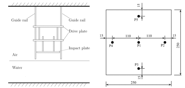
Fig. 3. Experimental configuration [21]. Left: side view of drop rig. Right: impact surface of the plate. Note: P1-P5 indicate the position of pressure transducers (all dimensions in mm). |
As the plate's impact surface is symmetrical about two planes, one-quarter of the computational domain was modelled with the solver's symmetry plane boundary conditions selected for the respective surfaces. Two geometrical regions were generated, namely the stationary background region, and the transient overset region surrounding the plate. To facilitate mesh refinement in critical regions of the model an overlap block was created to encompass the impact event, in conjunction with a free surface block to ensure the accurate representation of free surface behaviour. The geometrical coordinates of block corner extents are presented in Table 1. Note that the origin of the coordinate system is located at the still water line beneath the geometrical centre of the full plate. Boundary conditions for the model are presented in Table 2. The computational domain and locations of model blocks are illustrated in Fig. 4.
Table 1. Dimensions of computational domain. |
| Block | Corner 1 [m] | Corner 2 [m] | ||||
|---|---|---|---|---|---|---|
| x | y | z | x | y | z | |
| Background | 0 | 0 | -1.000 | 0.625 | 0.625 | 0.500 |
| Free surface | 0 | 0 | -0.060 | 0.625 | 0.625 | 0.060 |
| Overlap | 0 | 0 | -0.250 | 0.500 | 0.500 | 0.387 |
| Plate | 0 | 0 | 0.125 | 0.125 | 0.125 | 0.137 |
| Overset | 0 | 0 | -0.125 | 0.375 | 0.375 | 0.262 |
Table 2. CFD model boundary conditions. |
| Boundary name | Location | Type |
|---|---|---|
| Top | Upper surface of the computational domain | Pressure outlet |
| Bottom | Lower surface of the computational domain | No-slip wall |
| Far-field | Outer vertical surfaces of the Background block | Velocity inlet |
| Symmetry X | Background and Overset block x-z plane | Symmetry plane |
| Symmetry Y | Background and Overset block y-z plane | Symmetry plane |
| Overset interface | Shared Background-Overset region boundaries | Overset mesh |
| Plate | All plate surfaces | No-slip wall |
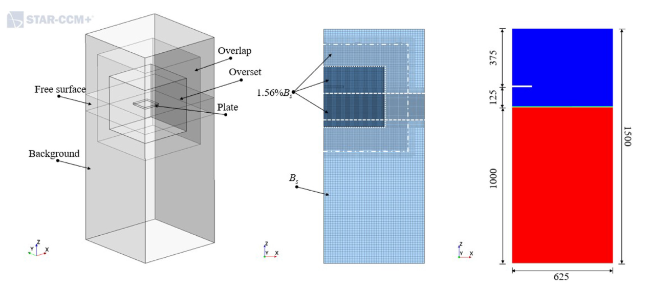
Fig. 4. Computational domain. Left: blocks and regions. Middle: mesh refinement regions as a percentage of base size. Right: initial VOF fractions, blue denotes air, red denotes water, plate shown in white (dimensions in mm). |
The trimmed cell mesher function with volumetric controls was used for all meshing operations except for surface controls for localised refinement on the plate surface. To ensure consistent transitions between mesh regions and optimal interpolation of solver variables, an equal mesh edge length was used for the overlap and free surface blocks (generated as isotropic), and all plate surfaces. Fig. 4 (middle) illustrates the level of each region's refinement as a percentage of a global mesh variable base size, Bs. Time series files of plate kinematics, impact force (Fz) and pressures are generated for each simulation. Numerical pressure data is recorded at points coinciding with the location of pressure transducers P1, P2 and P5 (Fig. 3) on the benchmark model plate's impact surface.
3.2. Flat plate with pocket models
Illustrated in Fig. 5, a central square pocket was modelled on the plate's impact surface, simulated in various dimensions of length, width, and depth (denoted as ΔL×ΔW×Δt). Several pocket configurations were created and tested. All simulation parameters except for this feature and the adjustment of vwere maintained as per the validation benchmark case discussed in Section 3.1. Table 3 details the dimensions of 22 pocket configurations numerically simulated.
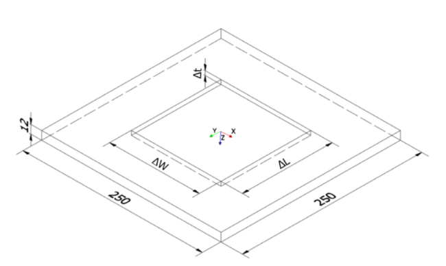
Fig. 5. The impact plate with void (pocket) of variable volume created on the impact surface (dimensions in mm). |
Table 3. Dimensions of pockets on plate impact surface. |
| ∆L or ∆W [mm] | ∆t [mm] | Volume [mm3] | ∆L or ∆W [mm] | ∆t [mm] | Volume [mm3] |
|---|---|---|---|---|---|
| 31.3 | 1.5 | 1465 | 125.0 | 6.0 | 93,750 |
| 62.5 | 1.5 | 5859 | 120.0 | 6.8 | 97,920 |
| 62.5 | 3.0 | 11,719 | 140.0 | 5.0 | 98,000 |
| 62.5 | 6.0 | 23,438 | 125.0 | 4.5 | 70,313 |
| 125.0 | 1.5 | 23,438 | 125.0 | 8.0 | 125,000 |
| 65.0 | 6.0 | 25,350 | 130.0 | 7.4 | 125,060 |
| 56.5 | 8.0 | 25,538 | 135.0 | 6.9 | 125,753 |
| 80.0 | 4.0 | 25,600 | 125.0 | 9.0 | 140,625 |
| 120.0 | 5.0 | 72,000 | 125.0 | 11.2 | 175,000 |
| 85.0 | 10.0 | 72,250 | 240.0 | 6.0 | 345,600 |
| 100.0 | 7.5 | 75,000 | 125.0 | 7.5 | 117,188 |
4. Results and discussion
4.1. Model verification and validation results
Simulation mesh uncertainty was quantified through the application of the generalised Richardson's extrapolation method, as outlined by [39]. A model with incompressible air and water phases was initially employed at a 100 μs time step (dt) for the following study, impacting the experimental model's velocity of 7 m/s. Three degrees of mesh coarseness were assessed using a Bs as the sole parameter modified between simulations, refined using a ratio of 2.0. Respective simulation results are summarised in Table 4 (see also Fig. 6), noting the peak pressure values at P2 and P5 are approximately identical due to the geometric symmetry (see Fig. 3). The relative error for each mesh size (total cell count) is presented in Fig. 7. All force and pressure results display monotonic convergence with a <1% error margin under the finest mesh arrangement relative to the coarse mesh indicating a stable, high-fidelity simulation. Under a medium mesh coarseness, P2 and P5 maintain a similar margin of error, Fmax and P1 results are within a 5% range. Due to the increased computational demand between medium and fine mesh cell count, a medium mesh coarseness is used in subsequent analyses.
Table 4. Mesh convergence study. |
| Mesh | Bs [m] | Cell count | CFL | Fmax [kN] | P1 [kPa] | P2 [kPa] | P5 [kPa] |
|---|---|---|---|---|---|---|---|
| Coarse | 0.48 | 649,833 | 0.09 | 35.2 | 805 | 483 | 482 |
| Medium | 0.24 | 4,759,790 | 0.19 | 45.7 | 1,035 | 619 | 616 |
| Fine | 0.12 | 36,470,179 | 0.37 | 47.3 | 1,076 | 620 | 616 |
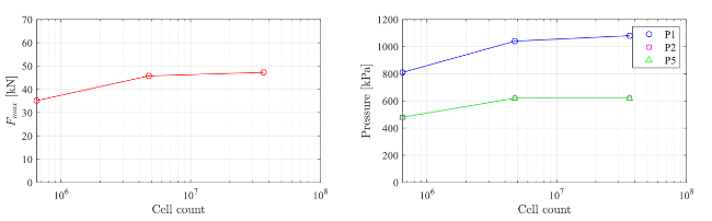
Fig. 6. Results of convergence study using total cell count at v = 7 m/s. Left: Convergence of impact force. Right: Convergence of impact pressures. |
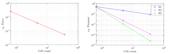
Fig. 7. Results of convergence study using total cell count versus relative error at v = 7 m/ s. Left: impact force. Right: impact pressure. Note: coarse mesh is the reference case for the convergence study. |
For validation of the model, a 20 μs time step (dt) is employed to match experimental pressure transducers’ sampling rate (i.e., 50 kHz). Numerical impact velocity is equal to the experimental value (7 m/s). Both air and water phases are modelled as compressible. Numerical and experimental results are presented in Table 5, time histories of impact force and P1 pressure are shown in Fig. 8. Both force and pressure plots show that secondary loading on the plate due to oscillatory behaviour of the air cushion is represented in the numerical model, however, the precise timing of these processes does not coincide with the experimental signals. The magnitudes of the CFD results are in good agreement with the experimental values (within 10% relative error) except for P5. Divergence of this pressure value may be attributed to an experimental irregularity; under ideal conditions, the geometrical similarity of this sensor's positioning (see Fig. 3) should return a magnitude that duplicates P2’s value. Interestingly, one also notes that the magnitude of slamming force and pressure is too sensitive to the time step (dt) being used in CFD simulations, e.g., 100 μs versus 20 μs (pressure peaks in Table 4 vs Table 5).
Table 5. Experimental and numerical results for impact force and pressures at v = 7 m/s. |
| Results | Fmax [kN] | P1 [kPa] | P2 [kPa] | P5 [kPa] |
|---|---|---|---|---|
| Experiment | 105.4 | 3762 | 1492 | 1073 |
| CFD | 99.1 | 4035 | 1348 | 1332 |
| CFD/Exp. [-] | 0.940 | 1.073 | 0.903 | 1.241 |
| Relative error, ϵR [%] | -6 | 7 | -10 | 24 |
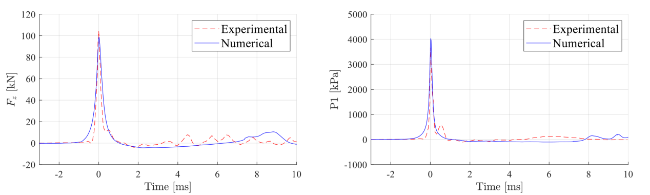
Fig. 8. Comparison of experimental and numerical results at v = 7 m/s. Left: slamming force. Right: slamming pressure at P1. |
The effect of the turbulence flow on the loading impact process with air pocket models was also conducted. To investigate the effects of turbulence occurring on the pocketed plate's surface upon impact, a k-ω SST model was simulated for numerous configurations of pocket geometry. Fig. 9 illustrates overlapping results for the 50% by proportion void (pocket size = ΔL×ΔW×Δt= 0.5 (L × W × tp) = 125 mm ×125 mm ×6 mm, W = B) for laminar flow and turbulence model for maximum plate pressure and plate centre pressure. Overall, the difference in fluid behaviour and results between laminar and turbulent fluid models was found to be negligible. Such a finding is consistent with previous studies on the numerical prediction of symmetric water impact loads on wedge shaped hull form [32]. Due to the instantaneous nature of the impact event, the flow is assumed as laminar for all the simulations and results reported hereafter.

Fig. 9. Time history of impact pressure using laminar flow and turbulence flow models for the pocket size at 50% of plate length, width, and thickness and impact velocity v = 7 m/s. |
4.2. Prediction of impact pressure
Numerical predictions of the maximum impact pressure (pmax) are compared with the theoretical estimations using the methods discussed in Section 2 for a range of impact velocity magnitudes (3-15 m/s). To maintain numerical validity, simulated impact velocities beyond the listed range were not attempted. The summary of such comparisons is given in Table 6. As shown in Fig. 10, there is a discrepancy among methods for the pmax prediction such that CFD results are lower than those of Von Karman method (calculated without consideration of the air cushion) and higher than those of Chuang method, and Okada & Sumi method. Results from the latter two methods display similar trends to one another throughout the tested range of v; Chuang predictions are consistently greater in magnitudes and closely approaching the numerical results at v = 3 m/s. At higher v values (> 12 m/s), the numerical results become closer to those estimated by the Von Karman method. The deviation between CFD and analytical/empirical results may be attributed to differences in experimental geometry, impacted masses and tested v values. At the highest velocity tested (v = 15 m/ s) CFD results approach Von Karman values, potentially proving that at a large impact momentum the effects of the air cushion may be negligible. Contrary to the various theoretical of shock pressure prediction, the non-linear gradient of the numerical values implies that pmax= (constant) ×v2, as shown in Fig. 10.
Table 6. Comparison of numerical and theoretical results of maximum impact pressure (pmax). |
| v [m/s] | CFL | CFD [kPa] | Chuang [kPa] | Okada and Sumi [kPa] | Von Karman [kPa] |
|---|---|---|---|---|---|
| 3 | 0.02 | 354 | 289 | 128 | 4339 |
| 5 | 0.03 | 1364 | 482 | 300 | 7232 |
| 7 | 0.04 | 4035 | 674 | 527 | 10,125 |
| 9 | 0.05 | 6956 | 867 | 802 | 13,018 |
| 15 | 0.08 | 19,986 | 1445 | 1885 | 21,697 |
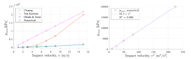
Fig. 10. Left: comparison of theoretical and numerical predictions of pmax. Right: relationship between v2 and pmax with line of best fit 91.7v2, R2 = 0.999. |
4.3. Influence of volume fraction
The results of this section were obtained at the impact velocity v = 7 m/ s for the flat plate as well as the flat plate with pocket models. CFD snapshots at different time instants were captured and discussed to highlight the loading impact process and the role of air entrapment which is represented by the volume fraction of air/water phases. Overall, the CFD tool facilitated the analysis of the complex loading processes occurring during fluid impact slamming through observation in a spatiotemporal sequence. Air entrapped on the plate's impact surface has been tracked using results from the VOF method's phase volume fraction feature and compared to a pressure profile of the impact surface. As the plate approaches the water free surface prior to impact, a layer of air becomes entrapped between solid and fluid and compresses at the plate's centre. As shown in Fig. 11, the largest magnitude of pressure in the impact event occurs at a 95% water volume fraction in which the compressed air (∼ 5% volume fraction) created the shock pressure spike on the plate's surface (at t = 17.88 ms). Fig. 12 shows a series of snapshots detailing the expansion of air layer post the impact event at different solution times (t = 18.88 ms and t = 19.88 ms). Fig. 13 illustrates the post-impact process ∼8 ms after the maximum magnitude of shock pressure (t = 26.22 ms) in which continuing a downward trajectory through the water medium, the air expands and a volume of gas is vented; pressure values reduce and the remaining entrapped air recompresses, and the process is repeated. A secondary pressure spike was observed at the plate centre prior to propagation outward towards the plate edge, the ring of peak pressure is reflected by a volume fraction of water >90%.
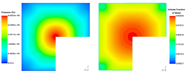
Fig. 11. Snapshots showing plate impact surface during maximum loading at t = 17.88 ms. Left: pressure distribution. Right: volume fraction of water. |
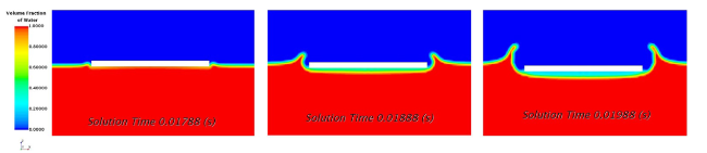
Fig. 12. Snapshots showing expansion of air layer post-impact at different solution times. Left: t = 17.88 ms (impact time). Middle: t = 18.88 ms. Right: t = 19.88 ms. |

Fig. 13. Snapshots showing pressure and volume fraction contours at t = 26.22 ms. Left: propagation of pressure wave on the plate surface. Middle: peak volume fraction of water on plate surface following pressure wave. Right: side view of water volume fraction. |
Fig. 14 shows the highest magnitude of slamming pressure on the plate's surface with a void (pocket) of 50% by proportion to plate length, width, and thickness i.e., ΔL×ΔW×Δt= 0.5 (L × W × tp). Unlike the flat plate impact, the pressure spike withing the modelled pocket is not symmetrical such that the largest magnitudes throughout the impact event do not occur exclusively at the plate's centre. The augmented area below the pressure curve indicates that the plate surface with air pocket is subjected to a greater magnitude of pressure impulse (∫p dt) during the slam event. It can be seen in Fig. 15 that the loading processes of the flat plate with air pocket differ by an ∼80% increase in pmax in comparison with the flat plate case (∼7100 kPa vs 4000 kPa) and occurring at a smaller volume fraction of water (88% vs 95%) i.e. larger air content entrapped (∼12% vs 5%). As shown in Fig. 16, after the initial pressure spike (t = 18.5 ms), the volume of the compressed air layer oscillates, first expanding then recompressing to impart a secondary pressure spike of approximately 750 kPa (see Fig. 17) at t ∼ 30 ms (∼11 ms after the primary loading). The volume fraction of water at this secondary loading event is ∼40%, indicative of a greater volume of entrapped air than the flat plate case (∼60% vs ∼5% volume fraction of air).
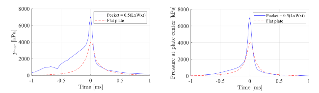
Fig. 14. Initial impact pressure spike Left: peak pressure magnitude for entire plate surface. Right: pressure at plate centre. |
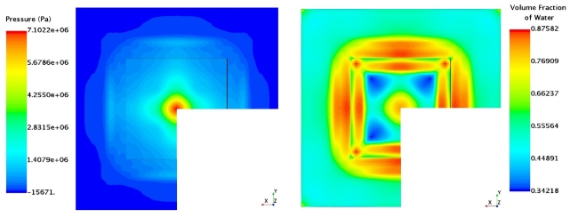
Fig. 15. Snapshots showing the plate impact surface during maximum loading at t = 18.5 ms. Left: pressure distribution. Right: volume fraction of water. |
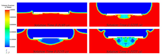
Fig. 16. Snapshot showing the volume fraction of water at different solution times from t = 18.5 ms (impact time) to t = 35.5 ms. |
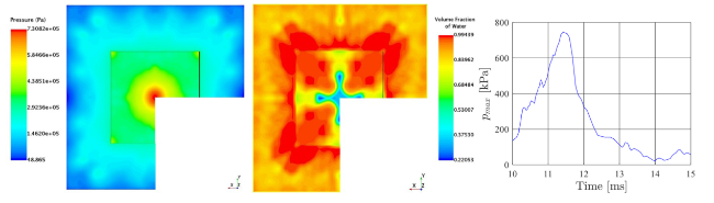
Fig. 17. Secondary pressure spike at t = 30.04 ms. Left: pressure distribution. Middle: volume fraction of water. Right: pmax time history of secondary peak. |
A comparison of three pocket depths (12.5%tp, 25%tp and 75%tp) at the instant of maximum loading is shown in Fig. 18. Visible are the differing shapes of entrapped air behaviour upon the impact; the shallowest pocket has the lowest volume of air and experiences the greatest loading of both pressure and force (pressure and force coefficients, Cf and Cp are explained in Section 4.4). The cushioning effect provided by the deepest pocket reduces both forms of loading significantly, achieved through compression inside the pocket and air expelled from this cavity cushioning non-pocket surfaces.

Fig. 18. Snapshots showing the interaction between the impacting plate and air-water mixture at the time of maximum loading at v = 7 m/s for various pocket depths and volumes. |
4.4. Parametric study into pocket geometry
The inclusion of a void (pocket) on the plate's impact surface was proven to influence slamming force and pressure results. The cushioning effect was found to be caused by the compression of a volume of air within the pocket, and air expelled from the pocket adding to the layer between non-pocket plate regions and the free surface of the water phase. In this section, the slamming force and pressure maxima are converted to coefficient form given in Eqs. (10) and 11, respectively, as
$C_{f}=\frac{2 F_{\max }}{\rho_{\text {fluid }} B^{2} v^{2}}$
$C_{p}=\frac{2 p_{\max }}{\rho_{\text {fluid }} v^{2}}$
Pocket depth, area and volume are non-dimensionalised as percentage values of the respective plate parameter, %tp, %ap and %volp. Overall, numerical results indicated that the presence of a pocket on a flat impact surface has the explicit effect of reducing slamming force which can be attributed to the cushioning effect of air within the void. The compression of this entrapped air has been shown to peak in pressure at a specific (critical) volume for a given impact velocity. Quantitative analyses into the effect of the pocket size on Cf and Cp are given below.
For comparative purposes, validation case coefficient results (v = 7 m/s) are Cf = 62.3 and Cp = 158.5, and a v = 3.5 m/s the flat plate (non-pocket) impacts returns Cf = 41.3 and Cp = 95.3 (represented by horizontal dashed lines in Fig. 19-Fig. 21). Fig. 19 displays a constant pocket void area with changing the pocket depth parameter alone. Resultant Cf values display a clear negative response to a deeper pocket. Both simulated impact velocities have a similar Cf floor value of ∼20 at depths >50%tp. Cp values increase up to 25%tp and decrease past this point. Unlike v = 7 m/s, 3.5 m/s results gradually reduce in a defined sequence all of which are lower in value than the flat plate's Cp result.
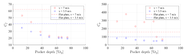
Fig. 19. Pocket depth effect on plate loading. Left: force coefficient. Right: pressure coefficient. |
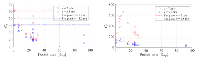
Fig. 20. Pocket area effect on plate loading. Left: force coefficient. Right: pressure coefficient. |

Fig. 21. Pocket volume effect on plate loading. Left: force coefficient. Right: pressure coefficient. |
Similar analysis was performed into the effects of the pocket area on loading such that as the pocket area increased, force values reduced. Fig. 20 displays %ap results employing a combination of depths, noticeable in both plots are the occurrence of multiple values of impact force and pressure for the same pocket area.
Coefficient results in Fig. 21 are from a combination of pocket depths and areas. Cf diminishes with an increase in volp (%) with a floor value of ∼20 for results >15%volp. Similar to Fig. 20, the data presents multiple resultant Cf values for an equal %volp and impact velocity. Visible in both graphs is the lower v value displaying a more consistent grouping of results. Pressure results indicate peak value occur for both velocities at ∼3.5%volp. Pressure coefficient values in Fig. 21 also parallel those of the pocket depth (Fig. 19); recorded pressures increase with an augmented pocket volume until reaching a critical volume, similar for both tested velocities. At volumes greater than the critical value, compression of entrapped air within the pocket reduces, and consequentially magnitudes of shock pressure also.
With further enquiry and refinement, results from future findings could be directly applied to the engineering design of structures. Where practical, the inclusion of a pocket on an impact surface of volume larger than the critical volume has the potential to reduce both slamming force and shock pressure to magnitudes lower than those experienced by a flat impact surface. Under the correct configuration of pocket volume and anticipated impact (or water particle) velocity, force and pressure magnitudes could be minimised allowing for greater factors of safety in design.
A comparison was made between the numerical prediction of pmax obtained inside the air pocket with the estimations of Bagnold and Mitsuyasu methods (refer to Section 2, Eqs. (5) and (6)). Following the recommendations of Takahashi et al. [34] for the fluid kinetic length parameter, K=πB/8, in which B is the impact length/width of the plate taken similar to [28], D is taken as the pocket depth and U=v, the non-dimensionalised peak pressures (pmax/p0) for all simulation results are compared to both theories as shown in Fig. 22 (noting the numerical predictions of pmax were normalised by the atmospheric pressure p0). Although the numerical results fall greater than both pmax/p0 domains of validity, the grouping of both methods appears predominately linear in comparison to CFD values (the four visible outliers are from 12.5%tp results). It should be noted that the numerical results exceeded the compression limits of both methods i.e., ppeak/p0 which are [0.8,4] for Bagnold's formula and [0.7,1.3] for Mitsuyasu's formula. Nevertheless, the CFD predictions for the tested geometries of the air pocket and impact velocities were found to follow the trend of Mitsuyasu's method (Eq. 6).
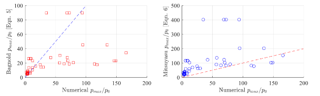
Fig. 22. Comparison of wave pressure prediction theories to numerical results. Left: Bagnold method (Eq. (5)). Right: Mitsuyasu method (Eq. (6)). Note: gradient of dashed line in both plots is 1:1. |
The results discussed in Section 4 have demonstrated the capability of the developed methodology in comparison with recent publications on water entry problems such as [26,29]. Main points include: (i) through a systematic parametric study into the size of air pockets, the developed methodology has enabled the quantification of the effect of air entrapment on the magnitude and distribution of slamming forces and pressures. (ii) CFD simulations showed that the cushioning effect of air during the entrapment causes the air to be compressed inside the pocket and later expelled from it, creating a layer between the bottom surface of the structure and the water. (iii) the resultant loads due to this interaction diverge from the simple water entry problems due to air effects and it will later alter the prediction of loads in a full-scale scenario as the conventional similitude laws (i.e., Froude's law) cannot be applied and hence CFD tools can be used to minimise such scale effects.
Finally, slamming events on a solid surface resulting from water entry have been proven complex processes upon consideration of object geometry and phase compressibility. Further research into slamming process parameters is recommended. To suitably validate the CFD model, an experimental prototype with a pocket on the impact surface should be constructed and tested at several impact velocities, with the capability of adjustable mass to observe its effect (if any) impact loading results. CFD testing of a pocketed model could be expanded to be subjected to wave impact, to assess the effects of air entrapment on offshore platform deck plating and girders. Due to the complexity of the phase interface in slamming events such as those simulated in this study, limitations that exist with VOF solvers may affect results. The VOF model does not explicitly track the interface, but rather reconstructs it based on individual cell volume fractions. The use of a different numerical solver to capture phase interface processes such as the Level Set (LS) method could provide more reliable computation of the phase phenomena associated with slamming events.
5. Conclusions
Numerical investigations into water entry problems of a rigid flat plate with air pockets were systematically conducted. The VOF model was utilised to capture localised slamming phenomena that occur during, and post-impact events. The model's geometry was modified to include a pocket on the slamming impact surface to investigate the effect of air entrapment on the magnitude and distribution of slamming forces and pressures. A parametric study was conducted on the geometry of the modelled pocket by altering its area, depth, and volume to examine the response of slamming and pressure loading under several impact velocities. The numerical slamming force and pressure results were compared with experimental drop test measurements and various theoretical methods of shock pressure predictions. Based on the results presented in this paper, the following conclusions can be drawn:
1. Overall, the functionally verified CFD model of a flat plate has successfully replicated an experimental drop test slam event. The numerical results of slamming forces and pressures were in good agreement with experimental drop test measurements with relative error of -6% and 7% for the magnitude of slamming force and pressure, respectively.
2. The numerical predictions of the maximum impact pressure (pmax) were larger than those estimated by the Von Karman method and samller than the values of Okada & Sumi, and Chuang. At the lowest impact velocity simulated, the numerical pressure results were approximately similar to the estimated values by Okada & Sumi, and Chuang. However, deviation at magnitudes was noticed at higher impact velocity which may be attributed to the geometric discrepancies, increased impact mass, and validated velocity ranges being used among methods. The difference in these parameters might alter impact momentum and geometrical (and possible phase) formation of the air cushion. Contrary to all theoretical methods, the relationship between shock pressure result maxima and impact velocity is not linear; the numerical results prove that peak pressure is proportional to the magnitude of impact velocity squared (pmax∝v2).
3. It was found that air became entrapped between the plate surface and the free surface of the water phase and compressed upon initial impact. The phase volume fraction at the point of maximum loading was <5% air by volume, coincident with a localised pressure spike on the plate's geometrical centre. Further observation of compressed air behaviour displayed oscillations in volume. A secondary pressure peak occurred during recompression; expansion of the air bubble was reflected by a ring of high pressure.
4. Unlike the flat plate impact, pressure maxima associated with air pocket models did not occur exclusively at the plate's centre during the initial impact shock event. Consequently, the impact area was subjected to a higher-pressure impulse and the formation of air cushion reduced the magnitude of impact force on the plate. Compression of the entrapped air was shown to increase peak pressure values by ∼80% in a pocket 50% of plate length, width, and thickness with a secondary peak observed at 10% of the initial slamming pressure magnitude for this model.
5. A study into the effects of pocket depth on loading results showed a noticeable trend of diminishing slamming force for deeper pockets. The two impact velocities tested (v = 3.5 and 7 m/s) had a similar force coefficient for pockets deeper than 50% of the plate thickness. However, the correlation between force and pressure coefficients versus the pocket depth were more evident for the lower impact velocity tested (v = 3.5 m/s). For the higher impact velocity tested (v = 7 m/ s), pressure coefficient results displayed a less-defined trend sequence versus the pocket depth. For the pocket volume effect, pressure coefficient values demonstrated a peak in the vicinity of the plate impact area with a pocket area size of 10% re-affirming the pocket depth and area findings. Force coefficients reduced with an increase in the pocket volume with almost no further reduction beyond 15% of plate volume.
6. A comparison of Bagnold's and Mitsuyasu's wave impact pressure prediction formulae showed a relationship between both approaches and the numerical results of pmax. It should be noted that the input to account for the entrapped air in either theorem is of the air cushion depth (D) alone, the use of different pocket volumes due to varying pocket areas is likely to affect results.
7. In comparison with recent investigations reported in the literature on water entry problems, the procedure and results of this paper showed how air entrapment can affect the prediction of slamming force and its pressure distribution and the formation of air cushioning during the entrapment which caused the air to be compressed inside the pocket and later expelled from it, creating a layer between the bottom surface of the structure and the water. The resultant loads due to this interaction diverge from the simple water entry problems due to air effects and it will later alter the prediction of loads in a full-scale scenario as the conventional similitude laws (i.e., Froude's law) cannot be applied and hence CFD can be useful tools to minimise such scale effects.
Declaration of Competing Interest
The authors declare that they have no known competing financial interests or personal relationships that could have appeared to influence the work reported in this paper.
Acknowledgements
The authors would like to acknowledge the National Centre for Maritime Engineering and Hydrodynamics of the Australian Maritime College for facilitating this study.
