
1. Introduction
Generally, traditional fish cages are used in nearshore seas and are small. The most widely used gravity cage, for example, mainly includes flexible nets and circular floating collars made of high density polyethylene (HDPE). The diameter of the floating collar is generally only 20-80 m [1]. Gravity cages have problems with net deformation due to strong waves and currents, and floating collars that may cause twisting problems [2]. In addition, pollution in the nearshore sea and the demand for high-quality fish products [3⇓-5] have prompted the steady development of aquaculture in the deep sea [6]. To meet the needs of high-quality and green fisheries [3⇓-5], various types of deep-sea aquaculture structures have been developed. Vessel-shaped fish cages are a new type of very large aquaculture structure designed for the open sea, that combines a very large floating body and aquaculture nets [1]. The robust and large steel structure can effectively adapt to the extreme environment in the open sea.
The floating body of a vessel-shaped fish cage, which is hundreds of meters long, is a typical ultralong floating structure, and the study of the hydroelasticity response is necessary. For very large floating structures, the hydroelasticity theories in the frequency domain, including the direct method [7] and the modal superposition approach [8,9], are widely used [10,11]. However, these theories are generally restricted to steady-state processes. For hydroelasticity theories in the time domain, two approaches have been developed [12], namely, the direct time integration method and the Fourier transform method based on Cummins' equation. The former method is time-consuming, and is suitable for strongly nonlinear problems. The latter is suitable for weakly nonlinear hydroelasticity problems and is computational efficient [13]. Based on the potential flow theory and Cummins' equations, Wei et al. [14] first discretized a continuous floating structure into multimodules connected by elastic beam elements, and then proposed a time-domain hydroelastic method for very large floating structures in inhomogeneous waves.
The hydroelasticity response of the frames/collars and net of fish cages has been widely studied. Fu et al. [15] adopted an extended 3D hydroelasticity theory in the frequency domain to predict the dynamic response of 5 × 2 floating collars in regular waves. Li et al. [16] used beam elements and truss elements to simulate the hydroelastic response of an elastic floating collar and a flexible net, respectively, in a finite element model. Hu et al. [17] studied the hydrodynamic response of a gravity fish cage under wave-current conditions considering the hydroelasticity of the net and floating collars, and found that much higher mode orders are excited when the significant wave height increases. Based on potential flow theory and dynamic cable theory, Ma et al. [18] studied the hydrodynamic response of a vessel-shaped fish cage with three rigid floating bodies connected by hinge joints. Additionally, the connecting loads between different floating bodies were also studied. However, the influence of nets and slender frames has not been considered. For the vessel-shaped fish cage, the hydrodynamic response has been studied recently, with the floating body of the fish cage usually regarded as a 6°degree-of-freedom (DOF) rigid body [19⇓-21], but the hydroelasticity of the floating body was not considered. Nevertheless, the hydroelasticity of a very large floating structure might be important [14], and the effects on the wave field and hydrodynamic load on the net should be analyzed.
In the present study, a numerical method is proposed to evaluate the hydroelastic responses of a vessel-shaped fish cage under coupling waves. First, the continuous floating body is discretized into a rigid multimodule system for multibody hydrodynamic analysis in the frequency domain, and the transfer functions of the wave excitation force considering the interactions between different modules and the velocity field transfer function induced by the diffraction and radiation waves in the frequency domain are solved via potential flow theory. Then, in the time-domain calculation, the rigid modules are connected by the equivalent beams, which are determined by the cross-sectional parameters of the original main steel structure. The hydrodynamic loads of the floating body are transformed from the frequency domain solution. The nets and the steel frames are divided into different blocks and subsequently coupled to the corresponding rigid module to transfer the hydrodynamic loads on the slender members, which are calculated by a Morison equation. Finally, an iterative method [22] is applied to obtain the balanced motion of the multimodule system and the hydrodynamic loads on the nets and the steel frames. The vertical displacements, cross-sectional bending moment and shear force of the coupled hydroelasticity model are analyzed, and the results show that the effects of hydroelasticity of the vessel-shaped fish cage are prominent.
2. Numerical model of the vessel-shaped fish cage
Fig. 1 shows the model of the vessel-shaped fish cage, which consists of the main steel structure (a floating body and steel frames, shown in blue and orange in Fig. 1, respectively) and flexible nets in red. Six large aquaculture cages are distributed along the x-axis and connected to the frames. Table 1 [19,20] shows the main parameters of the cage. The origin of the global coordinate system oxyz is located at the still water surface coincident with the center of the bow of the floating body.

Fig. 1. Model of the vessel-shaped fish cage. |
Table 1. Geometry and material parameters of the vessel-shaped fish cage. |
| Parameters | Unit | Value | |
|---|---|---|---|
| Floating-body length, LF | m | 385 | |
| Floating-body breadth, BF | m | 60 | |
| Floating-body height/draft, TF | m | 20 | |
| Size, D1 | m | 5 | |
| Size, D2 | m | 8 | |
| Size, D3 | m | 4 | |
| Main steel structure | Young's modulus, ES | GPa | 206 |
| Poisson's ratio, μ | - | 0.3 | |
| Density, ρS | kg/m3 | 7850 | |
| Diameter, B1 | m | 1 | |
| Diameter, B2 | m | 2 | |
| Section size, B3 | m | 2 × 1 | |
| Section size, B4 | m | 1.5 × 1.5 | |
| Net | Side length, BN | m | 45 |
| Net depth, HN | m | 40 | |
| Twine diameter, DN | mm | 5 | |
| Twine length, LN | mm | 50 | |
| Young's modulus, EN | GPa | 113 | |
| Solidity ratio | - | 0.19 | |
3. Theoretical background
3.1. Motion equation of the floating body
3.1.1. Motion equation of a multimodule system in the frequency domain
The continuous floating body is discretized into a multimodule system including N modules, and local coordinate systems are established for each module, as shown in Fig. 2. The multimodule system has N modules. Considering the hydrodynamic interactions between different modules, the potential flow theory is used to obtain the wave excitation force transfer function, as well as the added mass A(ω) and damping C(ω) of the multimodule system.

Fig. 2. Coordinate system of the multimodule system. |
The motion equation of the multimodule system in the frequency domain can be expressed as:
where ω is the wave frequency, MF(n) and KF(n) are the mass and hydrostatic restoring stiffness matrix of module n (n = 1,…, N), respectively; A(nm) and C(nm) represent the added mass and damping matrix of module n induced by the motion of module m (n, m = 1,…, N), respectively; and MF(n), KF(n), A(nm) and C(nm) are all 6 × 6 matrices. $ \overline{\mathbf{F}}_{W}^{(n)}$ and $ \overline{\mathbf{u}}_{F}^{(n)}$ (6 × 1 matrices with complex form) are the first-order wave excitation force and displacement of module n (n = 1, …, N), respectively. The symbol - denotes a parameter in the frequency domain.
For simplicity, Eq. (1) can be rewritten as:
$ \left[-\omega^{2}\left(\mathbf{M}_{F}+\mathbf{A}\right)_{6 N \times 6 N}-i \omega \mathbf{C}_{6 N \times 6 N}+\left(\mathbf{K}_{F}\right)_{6 N \times 6 N}\right]\left(\overline{\mathbf{u}}_{F}\right)_{6 N \times 1}=\left(\overline{\mathbf{F}}_{W}\right)_{6 N \times 1}$
where MF and KF represent the mass and hydrostatic restoring stiffness matrix of multimodule system, respectively; A and C are the added mass and damping matrix of multimodule system, respectively; MF, KF, A and C are all 6 N × 6 N matrices. $ \overline{\mathbf{F}}_{W}$ and $ \overline{\mathbf{u}}_{F}$ (6 N × 1 matrices) are the first-order wave excitation force and displacement matrices of the multimodule system in the frequency domain, respectively.
3.1.2. Motion equation of the equivalent structural model in the time domain
In the time-domain calculation, the discretized modules, which are used for hydrodynamic load modeling, are connected by Euler-Bernoulli beams, as shown in Fig. 3. The equivalent beam serves as a backbone to which the rigid modules are attached. There are N-1 beam elements for the multimodule system with N modules. In the equivalent structural model, the rigid module n is modeled as node n, and the wave excitation force and radiation forces of module n are applied to the corresponding node n. The centroid of each module is located at the same height and on the x-axis of the floating body, which also coincides with the equivalent beam.

Fig. 3. Equivalent elastic model. |
Under a regular wave, the corresponding time-domain equation of Eq. (2) considering the structural stiffness of elastic beams can be written as:
$ \left\{\begin{array}{l} \left(\mathbf{M}_{F}+\mathbf{A}\right)_{6 N \times 6 N}\left\{\ddot{\mathbf{u}}_{F}(t)\right\}_{6 N \times 1}+\mathbf{C}_{6 N \times 6 N} \dot{\mathbf{u}}_{F}(t)_{6 N \times 1} \\ +\left(\mathbf{K}_{F}+\mathbf{K}_{S}\right)_{6 N \times 6 N} \mathbf{u}_{F}(t)_{6 N \times 1}=\mathbf{F}_{W}(t)_{6 N \times 1} \\ \mathbf{F}_{W}(t)_{6 N \times 1}=\left[\begin{array}{llll} \mathbf{F}_{W}^{(1)}(t)_{6 \times 1} & \mathbf{F}_{W}^{(2)}(t)_{6 \times 1} & \cdots & \mathbf{F}_{W}^{(N)}(t)_{6 \times 1} \end{array}\right]^{T} \end{array}\right.$
where MF, KF and KS represent the mass matrix, hydrostatic restoring stiffness matrix and structural stiffness of the elastic beams, respectively; A and C are the added mass and damping matrix, respectively; and they are all 6 N × 6 N matrices. FW(t) (a 6 N × 1 matrix) is the first-order wave excitation force in the time domain; FW(i)(t) (a 6 × 1 matrix) is the first-order wave excitation force of module i (i = 1, …, N), as determined by $ \overline{\mathbf{F}}_{W}^{(i)}$ in Eq. (1); and uF(t), $ \dot{\mathbf{u}}_{F}(t)$ and $ \ddot{\mathbf{u}}_{F}(t)$ (6 N × 1 matrices) represent the displacement, velocity and acceleration of multimodule system in the time domain, respectively.
Under irregular waves, the radiation forces in the time domain can generally be calculated by the convolution term [14]. In this paper, the radiation forces of the floating body in irregular waves are calculated by the state space method, which is essentially developed from the convolution term [22,23]. Therefore, the time-domain equation based on the state-space method [22,23], can be rewritten as:
$ \begin{array}{l} \left(\mathbf{M}_{F}+\mathbf{A}(\infty)\right)_{6 N \times 6 N}\left\{\ddot{\mathbf{u}}_{F}(t)\right\}_{6 N \times 1}+\left(\mathbf{K}_{F}+\mathbf{K}_{S}\right)_{6 N \times 6 N} \mathbf{u}_{F}(t)_{6 N \times 1} \\ \quad+\mathbf{Z}_{\text {Rad }}(t)_{6 N \times 1}=\mathbf{F}_{W}(t)_{6 N \times 1} \end{array}$
(1) wave excitation force. As shown in Fig. 3, the external loads of the module n act on the n- th node of the equivalent elastic beam. Airy wave theory is used in this study. Under a regular wave, the first-order wave excitation force FW(n)(t) of module n (n = 1, …, N) in Eq. (3) can be expressed in the time domain as:
$\begin{cases}\mathbf{F}_W^{(n)}(t)_{6\times1}=\left[\begin{array}{ccc}F_{W1}^{(n)}(t)&F_{W2}^{(n)}(t)&\cdots&F_{W6}^{(n)}(t)\end{array}\right]^T\\F_{Wj}^{(n)}(t)=\zeta_A\left|\bar{F}_{Wj}^{(n)}\right|\cos\left(\omega t+\theta_j^{(n)}-(kx\cos\varphi+ky\sin\varphi)\right)\end{cases}$
where $ F_{W j}^{(n)}(t)$ is the first-order wave excitation force of module n in the j-th (j = 1, 2, …, 6) DOF. $ \left|\bar{F}_{W j}^{(n)}\right|$ and θj(n)are respectively the amplitude of the first-order wave excitation force transfer function and the phase angle between the wave excitation force and wave elevation in the j-th (j = 1, 2, …, 6) DOF of module n. In addition, ζA refers to the amplitude of the regular wave at frequency ω, k is the wavenumber, φ is the wave angle, and kxcosφ+kysinφ is the position phase.
Irregular waves can be considered a superposition of a series of regular wave components. In this study, the JONSWAP spectrum is used:
$ S(\omega)=319.34 \frac{\left(H_{S}\right)^{2}}{T_{P}^{4} \omega^{5}}\left\{-\frac{1948}{\left(T_{P} \omega\right)^{4}}\right\} \gamma^{\exp \left[-\frac{\left(0.159 T_{P} \omega-1\right)^{2}}{2 \sigma^{2}}\right]}$
where TP is the spectral peak period, HS is the significant wave height, ω is the wave frequency, γ is the spectral peak parameter (set as 3.3 in this study), and σ is the spectral width parameter.
Under irregular waves, the wave excitation forces on module n (n = 1, …, N) in Eq. (4) can be considered a superposition of excitation forces under a series of regular wave components. These forces can be expressed in the time-domain as:
$\begin{cases}\mathbf{F}_W^{(n)}(t)_{6\times1}=\left[\begin{array}{cccc}F_{W1}^{(n)}(t)&F_{W2}^{(n)}(t)&\cdots&F_{W6}^{(n)}(t)\end{array}\right]^T\\F_{Wj}^{(n)}(t)=\sum_l^M\zeta_{Al}\left|\bar{F}_{Wlj}^{(n)}\right|\cos\left(\omega_lt+\theta_{lj}^{(n)}+\varepsilon_l-(k_lx\cos\varphi+k_ly\sin\varphi)\right)\end{cases}$
where FW(n)(t) is the first-order wave excitation force of module n (n = 1, …, N) under irregular waves, the subscript l is the frequency number at wave frequency ωl for irregular waves, M is the total number of regular wave components used in the irregular wave, and ωl refers to the l-th (l = 1, …, M) wave frequency. $ \left|\bar{F}_{W l j}^{(n)}\right|$ and $ \theta_{l j}^{(n)}$ are the amplitude of the first-order wave excitation force transfer function and the phase angle between the wave excitation force and wave elevation in the j-th (j = 1, 2, …, 6) DOF of module n at wave frequency ωl, respectively, ζAl and kl refer to the wave amplitude and wavenumber at wave frequency ωl, respectively, φ is the wave angle, klxcosφ+klysinφ and εl denote the position phase and the random phase angle of wave elevation at wave frequency ωl, respectively, ζAl can be determined by $ \zeta_{A l}=\sqrt{2 S\left(\omega_{l}\right) \Delta \omega}$, where S is the wave spectrum in Eq. (6), and Δω is the frequency interval used in the irregular wave.
(2) structural stiffness matrix of the equivalent structural model. To ensure that the deformation of the equivalent elastic beam is consistent with that of the original steel structure, the beam parameters need to meet the following criteria [24]:
$ \left\{\begin{array}{l} E_{e} A_{e}=E_{r} A_{r} \\ E_{e} I_{M y e}=E_{r} I_{M y r} \\ E_{e} I_{M z e}=E_{r} I_{M z r} \end{array}\right.$
where E, A, IMy and IMz are the elastic moduls, cross-sectional area, vertical inertia moment, and transverse inertia moment, respectively; EeAe, EeIMye and EeIMze represent the axial stiffness, vertical bending stiffness and transverse bending stiffness of the equivalent structural beam, respectively; and ErAr, ErIMyr and ErIMzr represent the axial stiffness, vertical bending stiffness and transverse bending stiffness of the original steel structure, respectively. The subscripts e and r denote the parameters of the equivalent structural beam and the continuous floating body, respectively.
Dividing the cross-section into k subsections, the i th (i = 1,…, k) subsection can contribute to the axial stiffness, vertical bending stiffness and transverse bending stiffness of the cross-section. Considerating the parallel axis theorem, the stiffness of the equivalent beams can be determined by revising Eq. (8):
$ \left\{\begin{array}{l} E_{e} A_{e}=\sum_{i=1}^{k} E_{r} A_{r i} \\ E_{e} I_{M y e}=\sum_{i=1}^{k} E_{r}\left(I_{M y i}+A_{r i} h_{y i}^{2}\right) \\E_{e} I_{M z e}=\sum_{i=1}^{k} E_{r}\left(I_{M z i}+A_{r i} h_{z i}^{2}\right) \end{array}\right.$
where Ari is the area of the i th subsection, IMyi and IMzi are the vertical inertia moment, and transverse inertia moment of the i th subsection, respectively, hyi is the vertical distance between the i th subsection centroid and the y-axis, and hzi is the vertical distance between the i th subsection centroid and the z-axis. The torsional stiffness relating with the rotation and torsional moment needs to be determined by a numerical method for the relevant frame structure. However, the case considered in this study does not involve torsional response.
Combined with the axial stiffness, bending stiffness and torsional rigidity, the element stiffness matrix kn of the equivalent elastic beam n in the local coordinate system can be obtained [25]:
$ \mathbf{k}^{n}=\left[\begin{array}{ll} \mathbf{k}_{n, n}^{n} & \mathbf{k}_{n, n+1}^{n} \\ \mathbf{k}_{n+1, n}^{n} & \mathbf{k}_{n+1, n+1}^{n}\end{array}\right]$
where kn is a 12×12 matrix, and kn,mq is a 6 × 6 matrix determined by the beam parameters in Eq. (8), the superscript q is the beam element number (q = 1, …, N-1), the subscript n is the first node of beam element q and the subscript m is the second node of beam element q (n, m = 1, …, N).
By overlaying the element matrix in Eq. (10), the structural stiffness matrix of the equivalent elastic beam in Eqs. (3) and (4) can be expressed as:
3.2. Loads on the nets and frames
The nets and the frames are typical slender structures, and the hydrodynamic loads can be solved by the Morison equation, where the velocities are determined by the coupling wave fields including the incident, diffraction and radiation waves.
3.2.1. Velocity field considering diffraction and radiation waves
The multimodule system can generate diffraction and radiation waves. Under a regular wave with a wave amplitude of ζAl, the water particle velocity vl in the coupling wave fields can be expressed as follows:
where vIl, vDl and vRl are the velocities induced by the incident, diffraction and radiation waves, respectively; ωl is the wave frequency; vIl-k, vDl-k and vRl-k are the velocity components of vIl, vDl and vRl in the k-direction (k = x, y, z), respectively; ζAl is the wave amplitude at wave frequency ωl; θIl-x, θDl-x, θRl-x are the phase angles between the wave elevation and velocity transfer function of the incident, diffraction and radiation waves in the x direction at wave frequency ωl, respectively; the superscript n denotes the module order (n = 1, 2, …, N), where N is the number of the modules; the subscript l is the wave frequency order; the subscripts x, y and z denote the component of the parameter in the x, y and z directions, respectively; the subscripts I, D and R denote the parameters of the incident, diffraction and radiation waves, respectively; the symbol | | denotes the amplitude of the parameter; j represents the DOF (j = 1, …, 6); vIl, vDl, vRl are the water particle velocities induced by the incident, diffraction and radiation waves, respectively; $ \bar{v}_{I l-x}$ is the component of the velocity transfer function induced by the incident wave in the x direction, $ \left|\bar{v}_{I l-x}\right|$ represents the amplitude of $ \bar{v}_{I l-x}$; and $ \bar{u}_{R l j}^{(n)}$ and $ \delta_{R l j}^{(n)}$ are the motion amplitude and the phase angle of the module n between the velocity field transfer function and motion of floating module n in the j-th (j = 1, …, 6) direction at wave frequency ωl, respectively. Similar to the above parameters in x direction, the other parameters in the equation represents the corresponding parameters in the y and z directions, respectively, and εl denotes the random phase angle of the wave elevation at wave frequency ωl.
Based on the linear superposition assumption, the water particle velocity in the velocity field considering diffraction and radiation waves under irregular waves can be expressed as follows:
$ \mathbf{v}_{\text {irre }}=\sum_{l}^{M} \mathbf{v}_{l}$
where virre is the water particle velocity under irregular waves, M is the total number of regular wave components used in the irregular wave, and the amplitude of the regular wave component ζAl can be determined by the wave spectrum S(ω), $ \zeta_{A l}=\sqrt{2 S\left(\omega_{l}\right) \Delta \omega}$.
3.2.2. Hydrodynamic loads on the net and frame
The nets are simulated by truss elements, and the frames are simulated by beam elements[22]. The hydrodynamic load on the frame and net twine per unit length df(t) can be calculated by the Morison equation:
$ \begin{array}{l} \begin{aligned} d f(t)= & C_{D} \frac{1}{2} \rho d\left|v^{n}(t)-\dot{u}^{n}(t)\right|\left(v^{n}(t)-\dot{u}^{n}(t)\right)+\rho C_{M} \frac{\pi d^{2}}{4} \dot{v}^{n}(t) \\ & -\rho\left(C_{M}-1\right) \frac{\pi d^{2}}{4} \ddot{u}^{n}(t), \text { for frame } \\ d f(t)= & C_{D} \frac{1}{2} \rho d\left|v^{n}(t)-\dot{u}^{n}(t)\right|\left(v^{n}(t)-\dot{u}^{n}(t)\right), \text { for net } \end{aligned}\\ \end{array}$
where d is the equivalent diameter; vn and $ \dot{u}^{n}$ are the normal components of the velocity of the water particle and the element, respectively; $ \dot{v}^{n}$ and $ \ddot{u}^{n}$ denote the normal components of the acceleration of the water particle and the element, respectively; and CD and CM are the drag and inertial coefficients, respectively. For the net element, the inertial force term is neglected [26]. For the beam element, the drag coefficients for circular and rectangular cross-sections are equal to 1.0 and 2.0, respectively. The inertial coefficient is set to 2.0 [27]. For the truss element, the effective outer diameters of the horizontal net and vertical net are 0.4 m and 0.9 m, respectively, which ensures the hydrodynamic loads on all the truss elements are equal to that on the real fish net.
3.3. Hydroelasticity analysis method of the vessel-shaped fish cage
3.3.1. Motion equation of the coupled hydroelastic model
As shown in Fig. 1, the net is connected to the steel frame by hinged connectors. Then the loads on the nets and the steel frames are transferred to the equivalent elastic beam by master-slave constraints between each module and the corresponding nodes of the steel frames. Finally, the net and steel frames are coupled with the motion response of the equivalent elastic beam, and consequently the coupled hydroelastic model of the vessel-shaped fish cage is thus established, as shown in Fig. 4. When considering the contribution of the net and the steel frames, the motion equation of the coupled cage model can be written as:
where MH and KH (6 N × 6 N matrices) are the mass matrix and structural stiffness matrix considering the contribution of steel frames, respectively; uF and $ \ddot{\mathbf{u}}_{F}$ (6 N × 1 matrices) represent the displacement and acceleration, respectively. FAll is the external force, FN is the contribution of the net loads, and FS is the contribution of the steel frame hydrodynamics. FE represents the external loads on the floating body, including the wave excitation force FW, the radiation force zRad accounting for the frequency-dependent terms only, the hydrostatic restoring force KHuF and the force induced by the infinite-frequency added mass term $ \mathbf{A}(\infty) \ddot{\mathbf{u}}_{F}$, all of which are 6 N × 1 matrices.

Fig. 4. Coupling model of the wetted part of the fish cage. |
In this paper, the wave excitation force is applied to the corresponding nodes of the equivalent model of the floating body, and the velocity field induced by the incident and diffraction waves is applied to the net and the steel frames. The motion response is yielded by solving the coupled equation of Eq. (15). Then, the amplitude and phase angle of the motion for every module can be determined by applying the fast Fourier transform (FFT). Subsequently, the coupling wave fields including incident, diffraction and radiation waves are established based on Eq. (11), and the updated motion response can be obtained by solving Eq. (15). Therefore, a numerical iteration method is established. In the (j + 1)th iteration, the obtained j + 1$ \overline{\mathbf{u}}_{F}$ is compared with j$ \overline{\mathbf{u}}_{F}$ obtained in the last iteration. For each module, if $ \left\|{ }^{j+1} \overline{\mathbf{u}}_{F}^{(n)}-{ }^{j} \overline{\mathbf{u}}_{F}^{(n)}\right\| \leq \varepsilon\left\|^{j} \overline{\mathbf{u}}_{F}^{(n)}\right\|$ at any wave frequency, the iterative process is terminated. Here, the constant ε is set to 0.05 [22].
3.3.2. Procedures of the hydroelasticity analysis
Fig. 5 shows the flowchart of the hydroelasticity analysis of the vessel-shaped fish cage: First, the transfer functions of the wave excitation force of the multimodule system and the velocity field induced by diffraction and radiation waves in the frequency domain are solved by potential flow theory. In the time-domain, the wave excitation force of the multimodule system is transformed from the frequency domain results, and the radiation forces are calculated by applying the added mass and damping directly or the state-space method. Subsequently, the coupling wave fields acting on the nets and the steel frames are constructed by the transfer functions of the velocity field, wave amplitudes and multimodule motion response, where the radiation wave contribution to the velocity field is jointly generated by each module of the multimodule system and can be determined by an iterative method. Then, the equivalent structural model is established by elastic beams, which are determined by the original steel structure. The nets and the steel frames are divided into different blocks, and then coupled to the corresponding equivalent beams by master-slave constraints. In this way, the coupled hydroelasticity analysis method of the vessel-shaped fish cage is established. The numerical analysis is mainly carried out with ABAQUS software secondary development, and the accuracy of the calculation method has been validated [22,28].

Fig. 5. Flowchart of the hydroelasticity response analysis of the vessel-shaped fish cage. |
4. Numerical results
4.1. Numerical validation
4.1.1. Validation of the equivalent structural model
According to a precalculation, the natural frequencies of the rigid modes (heave, pitch and roll displacements) are 0.029, 0.032 and 0.089 Hz, and the natural frequencies of the first three dry flexible modes (they are all vertical bending modes) are 0.228, 0.533 and 0.825 Hz, respectively. The natural frequencies of the equivalent model and the original steel structure are consistent. To validate the accuracy of the equivalent structural model, the deformation of the original steel structure model and the equivalent elastic beam in the z direction is compared. As shown in Fig. 6, the vertical deformations at different cross-sections are consistent under the two different models, which indicates that the equivalent parameters are correct.

Fig. 6. (a) Load condition and (b) deformation result of the original steel structure model and the equivalent elastic beam in the z direction. |
4.1.2. Validation of the motion response
The radiation force of the floating body under regular waves can be calculated by directly applying added mass and damping to the multimodule system, and the radiation force can be calculated by the state-space method under irregular waves (this method can also be used under regular waves). To validate the accuracy of the state space method, the heave motion responses obtained by these two different methods are compared, as shown in Fig. 7. The wave height, wave period and wave direction are 4 m, 15.8 s and 180 deg, respectively. The heave motion obtained by the state-space method matches very well with that transferred from mass and damping directly.
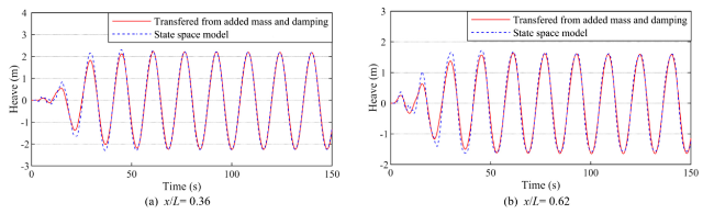
Fig. 7. Time series of the vertical displacements in the wave period 15.8 s and wave height 4 m. |
4.2. Results under regular waves
4.2.1. Time series of the main structure response
In this paper, only the wave direction of 180 deg is used due to the single point mooring system. Furthermore, due to the lack of detailed information, the vessel-shaped fish cage is still a simplified model. The cross-sectional stiffness of the main steel structure is set to K0 in this section. Fig. 8 shows the time series of the vertical displacement of the cage under the elastic model and rigid main structure (rigid model). The vertical motion of the rigid model decreases to some extent compared with that of the elastic model. With increasing x/L (from the cage bow to the cage stern), the difference in vertical displacement between the two model results decreases gradually, and they are almost identical at x/L = 0.94. Under the same external loads, the elastic model produces elastic deformation and subsequently leads to a more significant motion response than the rigid model.

Fig. 8. Time series of the vertical displacement at a wave height 19.2 m and wave period 15.8 s. |
Fig. 9, Fig. 10 show the time series of the cross-sectional shear force and vertical bending moment under the elastic model and rigid model, respectively. When the main structure is a rigid model, the cross-sectional load effect increases significantly. For the shear force, the increase at the cross-section near the cage stern is more pronounced. For the vertical bending moment, the influence of the rigid model shows the trend of “increasing and then decreasing” from the cage bow to the cage stern.

Fig. 9. Time series of the cross-sectional shear force at a wave height 19.2 m and wave period 15.8 s. |

Fig. 10. Time series of the cross-sectional vertical bending moment at a wave height 19.2 m and wave period 15.8 s. |
4.2.2. Effects of elasticity of the main structure on the net twine tension
To study the effect of elasticity on the net twine tension, the cross-sectional stiffness (namely, K0) used above is set as the reference in this section.
Fig. 11 shows the time series of the twine tension of the horizontal net element near the water surface at the cage bow, midship and stern. At the above three positions, the magnitude of the twine tension is not sensitive to the cross-sectional stiffnesses. Compared with the twine tension of the rigid model, the results for a smaller cross-sectional stiffness are slightly larger. This is because the motion response under a small stiffness is more prominent, and the hydrodynamic loads on the net are larger. Overall, the elasticity of the main steel structure has a limited influence on the net twine tension.

Fig. 11. Time series of the twine tension for a wave height of 19.2 m. (a) Twine tension at the cage bow. (b) Twine tension at the cage midship. (c) Twine tension at the cage stern. |
4.2.3. Effects of the elasticity of the main structure
For a more comprehensive analysis of the characteristics of the cross-sectional response, the cross-sectional stiffness (namely, K) of the main structure is changed by modifying the material elastic modulus, and the variation range of K is very large (although this seems difficult to achieve in reality). In this study, 6 different stiffnesses are used. Fig. 12(a) shows the vertical displacement amplitude at different cross-sections. With increasing x/L, the vertical displacement amplitude first increases and then decreases for smaller cross-sectional stiffnesses (K/K0<1). With increasing cross-sectional stiffness, the vertical displacement amplitude gradually decreases and reaches a steady state. This is because with the increase of cross-sectional stiffness, the contribution of the elastic deformation to the vertical motion response gradually decreases until it stabilizes to the rigid motion of the rigid model. At this time (steady state), the vertical displacement decreases linearly along the x-axis (from the cage bow to the cage stern). Fig. 12(b) shows the vertical elastic deformation under smaller cross-sectional stiffness. In the case of a smaller cross-sectional stiffness (such as K/K0=0.01), the elastic deformation presents a trend of "increasing and then decreasing" along the x-axis, which is consistent with the elastic deformation of the conventional hull along the x-axis. With increasing cross-sectional stiffness, the displacement amplitude decreases. When K/K0=0.01, the displacement amplitude is 5.3 m, and the displacement amplitude at the same cross-section is only 3.2 m when K/K0=1. In addition, the displacement amplitude at some cross-sections is almost twice that of the rigid model displacement when K/K0=0.01. This means that the vertical displacements of the cross-sections are very sensitive to the cross-sectional stiffness.

Fig. 12. (a) Vertical displacement amplitude at different cross-sections and (b) vertical elastic deformation under smaller cross-sectional stiffness. |
Fig. 13 and Fig. 14 respectively show the amplitude of the cross-sectional shear force and bending moment amplitude of the elasticity contribution at different cross-sectional stiffnesses. With increasing cross-sectional stiffness, the amplitudes of the shear force and bending moment increase sharply. As the stiffness continues to increase, the cross-sectional load effect stabilizes to a steady state. The increase in the cross-sectional load effect caused by the rigid model is substantial. At a stiffness of K/K0=0.01, the maximum shear force and bending moment amplitudes are 1.0e6 N and 1.0e8 N·m, while the amplitudes are 1.3e6 N and 2.4e8 N·m at a stiffness of K/K0=1, and the latter is 1.3 times and 2.4 times that of the former, respectively. This indicates that reducing the cross-sectional stiffness can significantly reduce the cross-sectional load effect of the cage.
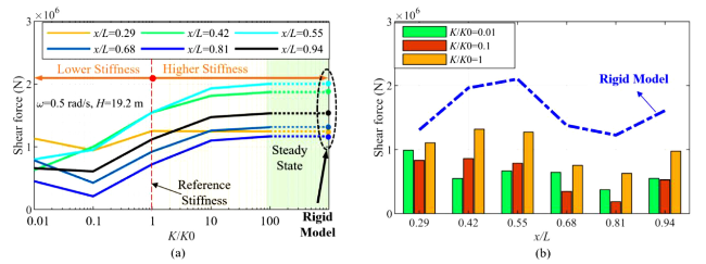
Fig. 13. (a) Shear force amplitude at different cross-sections and (b) shear force amplitude under smaller cross-sectional stiffness. |

Fig. 14. (a) Vertical bending moment amplitude at different cross-sections and (b) vertical bending moment amplitude under smaller cross-sectional stiffnesses. |
4.2.4. Results under different wave frequencies and wave heights
In this study, 4 different wave frequencies and 4 different wave heights are used, and the discrete results are obtained under these wave cases. Fig. 15 shows the vertical motion amplitudes of the vessel-shaped fish cage at different cross-sections. As the wave frequency increases, the vertical motion amplitude of the cross-sections near the cage bow (x/L<0.55) increases first and then decreases, while that of other cross-sections decreases. When the wave wavelength is equal to or slightly greater than the cage length, the vertical displacement is larger. The vertical motion amplitude increases gradually with increasing wave height. With increasing x/L, the vertical motion amplitude gradually decreases; that is, the vertical motion response from the cage bow to the cage stern gradually decreases.
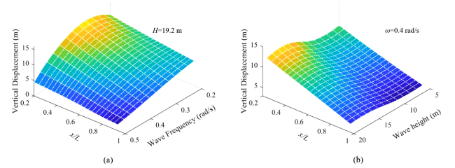
Fig. 15. Vertical displacement amplitude in different wave cases. (a) Results for different frequencies. (b) Results for different wave heights. |
Fig. 16 and Fig. 17 show the load effects on the cross-sections under different wave frequencies and wave heights, respectively. As the wave frequency increases, the cross-sectional shear force and bending moment gradually increase overall, but the results at some cross-sections have a maximum value at 0.4 rad/s, and the wavelength at 0.4 rad/s is close to the cage length. Taking the vertical bending moment as an example, the natural frequency of the first order vertical bending mode is 0.228 Hz, so the bending moment gradually increases as the wave frequency gradually approaches the natural frequency. The cross-sectional shear force and bending moment increase with increasing wave height, which is consistent with expectations.

Fig. 16. Cross-sectional force amplitude for different wave frequencies and a wave height of 19.2 m. (a) Shear force. (b) Vertical bending moment. |

Fig. 17. Cross-sectional force amplitude at different wave heights at a wave frequency of 0.4 rad/s: (a) shear force and (b) vertical bending moment. |
4.3. Results of different modules for the regular waves
To improve computing efficiency, the number of modules of the discretized multimodule system can be appropriately reduced. Fig. 18 shows the results under different numbers of modules. The reduction in the numbers of modules slightly reduces the vertical displacement amplitude of the cross-section. Compared with the result under seven modules, the vertical displacement amplitude decreases by 9% on average in the four-module model, while the shear force amplitude changes by 12% on average. The error is due to the difference in the number of modules and missing part of the characteristics of the main steel structure. However, the overall trend is consistent with the results under the seven-module model. To improve the calculation efficiency, the hydroelastic analysis under irregular waves in Section 4.4 is calculated by the four-module model.
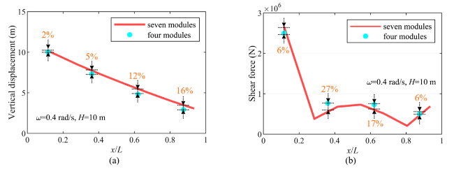
Fig. 18. Results under different number of modules. (a) Vertical displacement. (b) Cross-sectional shear force (default global stiffness K0). |
4.4. Results under irregular waves
In this section, the time series and the short-term extreme value of the response on the vessel-shaped fish cage is analyzed under irregular waves. The significant wave height and the peak period are 10.4 m and 15.7 s, respectively. To eliminate the transient effect, the duration of the simulation is set to 11000s, and 200 s time series are omitted to eliminate the transient effect. The response is assumed to satisfy the Weibull distribution [29], and the 99% fractile estimate value is chosen as the estimated extreme value [30]. In this section, only one seed is used for each irregular wave case. The identical wave elevation time series for the comparison between the elastic and rigid models is used, therefore, the uncertainty due to limited sampled size does not affect the comparison. In this section, the cross-sectional stiffness of the elastic model is the default global stiffness K0.
4.4.1. Motion response
Fig. 19 shows the time series of the vertical displacement at x/L = 0.5 under irregular waves. The same wave elevation series is used for the elastic model and the rigid model. The motion response of the rigid model is reduced under irregular waves, which is consistent with the results under regular waves. In addition, there is a main response period of 35 s, which is caused by the natural frequency of heave displacement. Fig. 20 shows the vertical displacement statistical results of different cross-sections under irregular waves. The extreme value and root mean square (RMS) value of the cross-section vertical displacement from the cage bow to the cage stern decrease gradually. The vertical displacement under the rigid model decreases prominently, and the average decrease in the extreme value and RMS values reaches 33% and 23%, respectively. On the one hand, the mooring system at the cage bow generates an additional force on the cage bow, on the other hand, the nets at the cage stern have a damping effect on the vertical displacement. Therefore, the motion response of the cage is similar to a beam with an elastic support at the stern and a concentrated force at the bow.
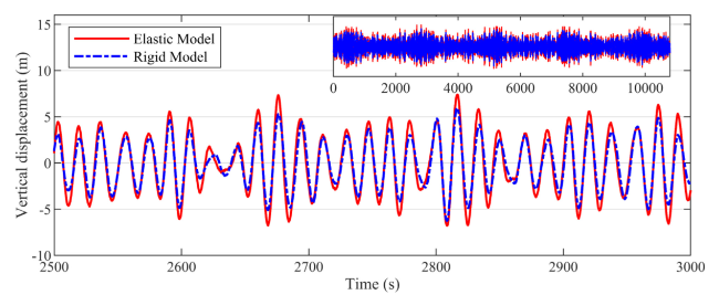
Fig. 19. Time series of the vertical displacement at x/L = 0.5 under irregular waves (default global stiffness K0). |
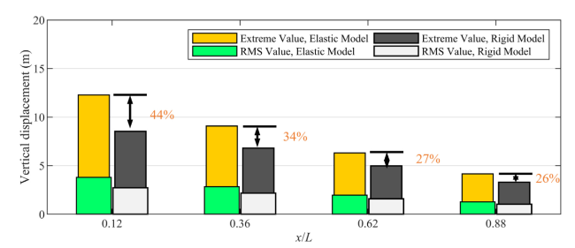
Fig. 20. Vertical displacement statistical results of different cross-sections under irregular waves (default global stiffness K0). |
4.4.2. Cross-sectional load effect
Fig. 21 and Fig. 22 show the time series of the cross-sectional load effects at x/L = 0.5 under irregular waves. The cross-sectional load effect under the rigid model changes prominently compared with that under the elastic model. Fig. 23 shows the load effect statistical results of different cross-sections under irregular waves. Compared with the shear force under the elastic model, the shear force under the rigid model increases slightly, and the average reduction in the maximum and RMS values is only 11% and 9%, respectively. For the bending moment, the average reduction of the maximum and RMS values under the rigid model is 41% and 40%, respectively. On the whole, the cross-sectional load effect under the rigid model is significantly larger than that of the elastic model, which is consistent with the results under regular waves.

Fig. 21. Time series of the cross-sectional shear force at x/L = 0.5 under irregular waves (default global stiffness K0). |
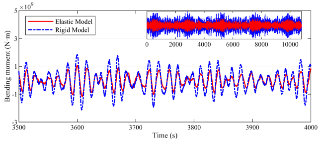
Fig. 22. Time series of the cross-sectional vertical bending moment at x/L = 0.5 under irregular waves (default global stiffness K0). |

Fig. 23. The statistical results of cross-sectional load effects under irregular waves (default global stiffness K0). (a) Shear force. (b) Vertical bending moment. |
5. Conclusion
In this paper, a novel time-domain method used in hydroelastic analysis of a vessel-shaped fish cage is proposed. First, the continuous floating body is discretized into a rigid multimodule system connected by equivalent elastic beams, and the hydrodynamic loads on the rigid multimodule, which are transformed from frequency-domain load coefficients, are applied to the corresponding nodes of the equivalent elastic beams. The coupling wave fields including the incident, diffraction and radiation waves are built, and then the hydrodynamic loads on the net and frame are calculated by the Morison equation. The model of the flexible net and steel frame are coupled with the equivalent elastic beams by master-slave constraints, and subsequently, the coupled hydroelastic model including the floating body, net and steel frame is established. Then, the coupling effect can be achieved through multiple numerical iterations. Finally, the hydroelastic response of the vessel-shaped fish cage under coupling wave fields is analyzed, and the following conclusions are reached.
(1) The vertical displacement of the cage decreases significantly under the rigid model at different cross-sections. With increasing x/L, the difference in vertical displacements under the elastic and rigid models decreases gradually. The cross-sectional shear force and vertical bending moment under the rigid model are larger than those under the elastic model. Therefore, the results of the rigid model are conservative; however, from the perspective of cost control, the elastic model can eliminate the structural redundancy and thus reduce the cost.
(2) With increasing cross-sectional stiffness, the vertical displacement of the cage gradually decreases and eventually stabilizes. The cross-sectional shear force and vertical bending moment increase significantly to constant values with decreasing stiffness. Overall, the cross-sectional stiffness has a limited influence on the net twine tension.
(3) Suitably reducing the number of multimodules improves the computational efficiency and maintains the overall accuracy of the hydroelastic response. By using the fewer-module model to calculate the hydroelastic response of the cage under irregular waves, the motion response and cross-sectional load effects of the rigid model change significantly compared with those of the elastic model.
Declaration of Competing Interest
The authors declare that they have no known competing financial interests or personal relationships that could have appeared to influence the work reported in this paper.
Acknowledgements
The authors gratefully acknowledge the National Natural Science Foundation of China (Grant No. 52088102), National Science Fund for Distinguished Young Scholars (Grant No. 51825903), the Fundamental Research Funds for the Central Universities, Key R & D program of Shandong Province (Grant No. 2021SFGC0701), National Natural Science Foundation of China (Grant No. 52271283 and Grant No. 52111530135), State Key Laboratory of Ocean Engineering (Shanghai Jiao Tong University) (Grant No. GKZD010081), Shenlan Project (Grant No. SL2021MS018 and Grant No. SL2022ZD201) and the Research Council of Norway through the centre of Excellence Funding Scheme (Grant No. 223254).
