
1. Introduction
In recent years, floating wind turbines attract great research interests and have huge potential for the future development of offshore wind energy. Many different floater concepts, including traditional spar (for example Hywind [1]), semi-submersible (for example WindFloat [2]) and TLP, as well as novel concepts of truss floaters (for example TetraSpar [3]), barges (for example Floatgen [4]), etc., have been proposed and developed into different levels of industrial and commercial maturity. Most of the floater concepts have a similarity as offshore oil and gas platforms and a comparative study about the advantages and disadvantages of the different floaters for floating wind turbines can be found in [5]. Among them, semi-submersibles, with three or four columns and with braces or pontoons [6], have the advantages to be deployed in waters with a relatively moderate water depth, between 50 m and 200 m.
Along with the development of floating concepts, numerical codes and software (FAST [7], HAWC2 [8], DNV SIMA [9], etc.) have also been developed with focus on global coupled wind and wave loads and responses analysis using a time-domain approach. Most of these codes are referred to as global load and response analysis codes, that can be used for engineering design of floating wind turbines. Their aerodynamics are based on the blade element moment theory with engineering corrections and their hydrodynamics are based on the potential flow theory for large-volume structures and the Morison's formula for slender components. The IEA OC3-OC6 benchmark studies focus on the software-to-software, software-to-experiment as well as software-to-field-measurement comparisons of these codes for different bottom-fixed and floating wind turbine concepts and present a very good summary of the theories in different codes as well [10]. Those codes are very efficient so that it is feasible to consider more than 15,000 one-hour or three-hour time-domain simulations that are typically required for engineering design checks.
In such global analysis tools, from the hydrodynamic loads modeling point of view, a semi-submersible floater might be modeled as one rigid body, or multiple rigid-bodies connected with beam-type braces, or multiple rigid-bodies connected with rigid beams in global analysis [11,12], from which the global motion dynamics of the floating wind turbines are easily obtained. It is common that the blades, tower and mooring lines are modeled as slender structures with distributed aerodynamic or Morison-type hydrodynamic loads, respectively, and the cross-sectional loads (and therefore induced stresses) of these components can be obtained directly from the time-domain simulations for design check. However, in order to do design checks for the floater with respect to ultimate and fatigue limit states, one has to obtain the stress distributions in the floater. The modeling approaches above can only provide the cross-sectional loads if the structural components are modeled as beams, but they cannot provide the detailed stress results of the floater structural components, such as hull plate, stiffeners, bulkheads, etc. For these structures, a regeneration of the hydrostatic and hydrodynamic pressure loads is needed and should be applied using a shell finite element-based model for stress analysis. There are also methods that were developed to consider hull flexibility for TLP wind turbines [13], which are important for ultra large wind turbines. In addition, experimental methods have also been developed to measure the cross-sectional loads on rigid floaters [12] and flexible floaters [14] for wind turbines.
For design of offshore floating oil & gas platforms, a frequency-domain-based hydrodynamic and structural analysis method and procedure have been developed by DNV and implemented in their SESAM software package, the frequency-domain hydrodynamic software DNV WADAM [15] and the structural analysis software DNV SESTRA [16]. From such analysis, stress transfer functions due to regular wave actions for the whole floater structural components can be obtained and used for design checks in combination with irregular wave conditions. However, such methods (based on the regeneration of wave pressure loads) have not be implemented for time-domain simulations, which are typically carried out from the global analysis point of view. Alternatively, time-domain hydrodynamic codes (such as DNV WASIM [17]) might be used to obtain the detailed pressure loads when the global motions of the floating wind turbine are known [18]. This approach has been used for design of the OO Star semi-submersible floating wind turbine [19]. However, such methods are very time-consuming and might not be suitable for efficient estimation of floater stresses for fatigue design analysis.
In this paper, an analysis procedure is developed to regenerate the time-varying hydrostatic and hydrodynamic pressure on the external wet surface of the floater using the irregular waves and floater motions from a global analysis as input. These pressure loads are further applied on a shell finite element-based structural model, together with the time-varying gravity, the inertial loads, the loads at the tower bottom and mooring line fairleads of the floater for stress analysis. This procedure is verified against the frequency-domain regeneration of the stress results, considering irregular wave actions.
2. The EMULF project and the 15MW semi-submersible wind turbine
The EMULF project, Efficient Numerical Modelling Methods for Design and Analysis of Ultra-Large Floating Wind Turbines, 2021.01-2022.06, is a joint project between COWI, NTNU, DTU and DNV, with the financial support from COWI Fonden. The project deals with numerical modeling methods for both global analysis of floating wind turbines (FWTs) under simultaneous wind and wave loads and local structural stress analysis for design of the floater. The whole project mainly includes WPB FWT global integrated analysis considering floater flexibility using SIMA and HAWC2 software, WPC Validation of the floater flexibility on global dynamic responses against a two-body experiment under wave loads, WPD Time-domain stress analysis of the floater, WPE Frequency-domain stress analysis of the floater and WPF Comparison of frequency-domain and time-domain global dynamic analysis. In this paper, the methodology and the results from WPD will be presented.
The initial design of a semi-submersible floater developed by the University of Maine (UMaine) to support the IEA 15MW wind turbine was used in this project. Fig. 1 shows an illustration of the floating wind turbine with the catenary mooring system. In the analysis in this work, the wind and wave direction of 0°, from left to right on the right plot, is considered. The main dimensions of the turbine and the floater are listed in Table 1 and Table 2, and more details can be found in [20] and [21].
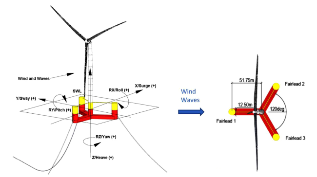
Fig. 1. Illustration of the UMaine semi-submersible with the IEA 15MW wind turbine ([14], left: overview; right: bird view). |
Table 1. Main features of the IEA 15MW wind turbine [20]. |
| Parameter | Value | Unit |
|---|---|---|
| Rated power | 15 | MW |
| Control | Variable speed, collective pitch | |
| Cut-in, rated, cut-out wind speed | 3, 10.59, 25 | m/s |
| Minimum, maximum rotor speed | 5, 7.56 | rpm |
| Rotor diameter | 240 | m |
| Hub height | 150 | m |
| Blade mass | 65 | ton |
| Rotor nacelle assembly mass | 1017 | ton |
| Tower mass | 860 | ton |
Table 2. Main dimensions of the UMaine semi-submersible [21]. |
| Parameter | Value | Unit |
|---|---|---|
| Displacement | 20,711 | ton |
| Floater steel mass | 3914 | ton |
| Draft | 20 | m |
| Side column freeboard | 15 | m |
| Central column diameter | 10 | m |
| Side column diameter, length | 12.5, 35 | m |
| Distance between central and side column centres | 51.75 | m |
| Pontoon height, width | 12.5, 7 | m |
| Vertical position of CoG from SWL | −14.94 | m |
| Vertical position of CoB from SWL | −13.63 | m |
| Water depth | 200 | m |
| Mooring system | Three catenary chain lines | |
| Surge natural period | 143 | s |
| Sway natural period | 143 | s |
| Heave natural period | 20.4 | s |
| Roll natural period | 27.8 | s |
| Pitch natural period | 27.8 | s |
| Yaw natural period | 90.1 | s |
| 1st tower bending natural period (fore-aft) | 2.02 | s |
| 1st tower bending natural period (side-to-side) | 2.07 | s |
3. General methodology for floater stress analysis
A global analysis of a floating wind turbine needs to be performed first, in which the coupled dynamics (in terms of rigid-body floater motions) are solved when the floating wind turbine is under simultaneous wind and wave loads. The modeling approach and details can be found in [22] using SIMA. Then, a structural stress analysis is performed.
The basic idea to do stress analysis for a floating wind turbine is, based on the global analysis results (time series of floater motions and loads at the tower bottom and the mooring line fairleads), to reconstruct all the applied distributed loads, which include both the external environmental loads (due to wind and waves) and the inertial loads, and to apply them on a finite element (FE) model for quasi-static stress analysis. The applied loads will be in equilibrium for each time step as in the global analysis, while the deformation and stress results will be calculated from this quasi-static structural analysis. It should be noticed that in the structural analysis, global floater motions are not solved again, and they are known and considered as input for structural analysis. From the global analysis point of view, the distributed hydrodynamic pressure on each panel will result into the same global load effect as the integrated hydrodynamic pressure, in terms of the forces and the moments in 6 DOFs or multi-DOFs for the floater.
Fig. 2 shows the analysis procedure for the floater stress calculation. The focus of this paper is to develop a code that can regenerate the time series of all the applied loads (especially the hydrodynamic wave pressure loads) on the floater (as shown in blue), which are used in a finite element model for stress analysis (as shown in green). It should be noticed that the distributed hydrostatic/hydrodynamic pressure loads refer to a panel model, and need to be mapped to the FE model, which are realized using WASIM.
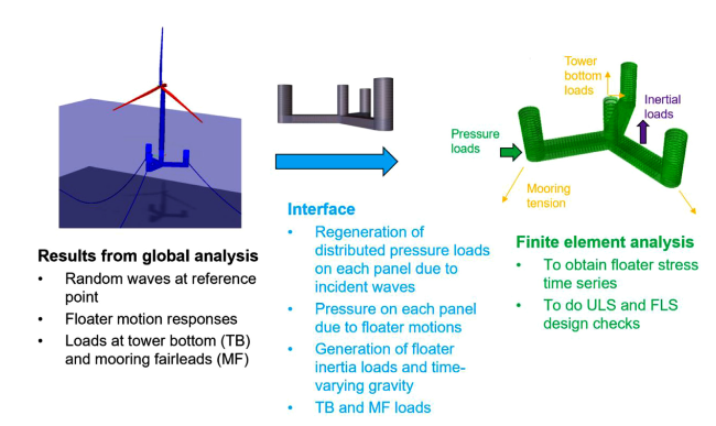
Fig. 2. Analysis procedure for reconstruction of the applied loads for floater stress analysis (left: the global model in SIMA; middle: the panel model in WADAM or WASIM; right: the finite element model in SESTRA). |
It should be noticed that the boundary conditions are introduced at three nodes of the FE model, with the constraints of fixed-fixed-fixed, fixed-fixed-free and fixed-free-free for translational degrees of freedom. The three nodes are taken on the bottom surface of the pontoons, which have no influence due to stress concentration for the selected positions for stress comparison. The structural analysis for each time step is performed using a local coordinate system, which is assumed to follow the global floater motions so that the time-varying gravity and buoyancy forces are also included.
The components of the external loads acting on the FE model (as shown in blue in Fig. 2, which can be built and analyzed using for example SESTRA are listed below and the way how their time series are obtained is also explained.
• Cross- sectional loads at the tower bottom and mooring line fairleads, which are obtained directly from the global analysis results in SIMA, since typically the tower and mooring lines are modelled as finite element beams and their cross-sectional loads are easily obtained.
• The time-varying gravity due to the floater rotational motions is included.
• The distributed inertial loads due to the acceleration of the floater are applied by considering the acceleration field of the floater due to motions.
• The inertial effects of the ballast water inside the pontoons and the columns are considered in a quasi-static method as time-varying dynamic pressure due to the ballast water acceleration, acting on the internal wet surfaces of the pontoons and the columns.
• Hydrostatic and hydrodynamic pressure loads on the external wet surfaces of the floater are applied and have many components as below. Table 3 shows how different pressure loads are obtained.
Table 3. Relationship between wave elevation and floater motion as input and the corresponding wave pressure as output. |
| Input | Output | Relationship |
|---|---|---|
| General input u(t) | General output y(t) | Transfer function HUY(ω) |
| Wave elevation at the reference point ζ(t) | Wave excitation pressure at panel j pje(t) | Transfer function HZPEj(ω) |
| Floater motion in DOF i xi(t) | Wave radiation pressure at panel j (added mass and potential damping terms) pjir(t) | Transfer function HXiPRj(ω) |
| Floater motion in DOF i xi(t) | Time-varying hydrostatic pressure at panel j pjis(t) | Transfer function HXiPSj(ω) |
• The time-varying hydrostatic pressure load on each panel due to the floater translational and rotational motions are included and expressed using a transfer function.
• Based on the wave radiation analysis, the wave radiation pressure is calculated using the transfer function between the floater motions and the wave radiation pressure at each panel, including both the added mass and the potential damping terms.
• Based on the wave diffraction analysis, the wave excitation pressure is calculated using the transfer function between the wave elevation at the reference point and the wave excitation pressure at each panel.
Table 3 shows the relationship between wave elevation and different components of hydrodynamic pressure on each panel based on a linear transfer function formulation. The general output in the table can be presented using the general input and the transfer function as below.
$ u(t)=\operatorname{Re}\left[\sum_{n=1}^{N} u_{n} \exp \left(i\left(\omega_{n} t+\varphi_{n}\right)\right)\right]$
$ y(t)=\operatorname{Re}\left[\sum_{n=1}^{N} u_{n} \operatorname{abs}\left(H_{U Y}\left(\omega_{n}\right)\right) \exp \left(i\left(\omega_{n} t+\varphi_{n}+\operatorname{pha}\left(H_{U Y}\left(\omega_{n}\right)\right)\right)\right)\right]$
Here the functions abs() and pha() represent the absolute value and the phase angle of the transfer function.
Several important assumptions are made and justified for this analysis procedure, which are discussed below.
• The gravity and the buoyancy forces when the floater is at the mean position are considered as static loads, which are applied directly on the FE model for the static stress analysis. Similarly, the effects of the ballast water inside the pontoons and the columns due to gravity are modelled as hydrostatic pressure on the internal wet sides of the pontoons and the columns [10]. The focus of this paper is on the dynamic responses and therefore these loads are not considered in the comparison.
• All the time-varying hydrostatic and hydrodynamic pressure loads are considered up to the first-order terms (with respect to wave elevation and floater motions, respectively) and are applied up to the mean external wet surface of the floater. Normally, the first-order pressure loads are much larger than the second-order or the higher-order pressure loads.
• The second-order hydrodynamic pressure (due to incident waves and wave-structure interactions) was not considered, which is typically much smaller than the first-order components. Hydrodynamic pressure due to viscous effects is also assumed to be small and therefore they are not included in the structural analysis. However, the second-order wave loads and the viscous effects can be considered in the global analysis to obtain the motion responses. The resulting second-order motions and their induced time-varying hydrostatic and hydrodynamic pressure loads can be included in the structural analysis. However, in the validation of the time-domain analysis procedure against the frequency-domain stress regeneration later in this paper, the second-order loads are not considered either in the global motion analysis, or in the structural analysis. The effects of the slowly-varying motions induced by the second-order wave loads and the wind turbine loads on the structural stresses will be investigated in the later study.
• Based on the WAMIT theory manual [23], the time-varying hydrostatic pressure load on each panel has two terms of the first-order contributions, because of the Taylor expansion about the load on that panel, as shown in Eq. (3). The first term is due to the hydrostatic pressure change caused by floater motions when the panel is at the mean position. The second term is related to the change of the normal vector due to rotational motions when the hydrostatic pressure is taken at the mean position. However, the second term results into an in-plane force vector that is normally very small. Therefore it is not considered in this study.
$ -\rho g \iint_{S_{j}} n\left(\eta_{3}^{(1)}+\alpha_{1}^{(1)} y-\alpha_{2}^{(1)} x\right) d S-\rho g \iint_{S_{j}}\left(\alpha^{(1)} \times n\right) z d S$
Here, n presents the normal vector of the panel j (Sj) at the mean position of the floater, η(1) and α(1) are the first-order transitional and rotational motion vectors, as in xi in Table 3. x,y and z are the coordinates of the centroid for the panel j, ρ and g are the water density and the gravitational acceleration.
4. Analysis procedure in the DNV software package
The methodology and the analysis procedure as shown in Fig. 2 will be illustrated using the DNV software package, which includes WADAM (or WAMIT) for frequency-domain hydrodynamic analysis, SIMA for global analysis of the floating wind turbine under wind and wave loads, and WASIM and SESTRA for floater load transfer and structural analysis. In addition, a MATLAB code is developed to reconstruct the different components of the hydrostatic and hydrodynamic pressure on each panel based on the methodology explained in Section 3. A brief explanation is given below.
• Step 1. WADAM (or WAMIT) is used to obtain the hydrodynamic coefficients for global analysis, which include the integrated wave excitation loads, added mass and potential damping coefficients, as well as the hydrostatic restoring coefficients, considering the 6DOF of the floater motions. The transfer functions of the wave excitation pressure and the wave radiation pressure for each panel are also obtained, which are used in Step 3 to reconstruct the pressure load time series. It should be mentioned that the separate wave excitation pressure and radiation pressure transfer functions are obtained from WAMIT in this study. In principle, WADAM can also output these results.
• Step 2. SIMA is used for global analysis of the floating wind turbine in which the floater is assumed to be one rigid-body with 6DOF of motions. Rotor, tower and mooring lines are modeled using a finite element method. Therefore, the motion responses due to the simultaneous wind and wave loads are obtained, considering turbulent wind and irregular waves. Moreover, the tower bottom cross-sectional loads and the mooring line tension at the fairleads are also obtained. The wave elevation time series at the reference point are also saved for the use in Step 3.
• Step 3. Using the developed MATLAB code, the time-varying hydrostatic and hydrodynamic pressure time series for each panel are generated and transferred via WASIM to a shell-based finite element model of the floater in SESTRA. The transferred loads also include the time-varying gravity loads, the inertial loads of the floater, the tower bottom loads and the mooring line loads using the available features in WASIM.
• Step 4. A linear structural stress analysis is then performed in SESTRA for each time step and the stresses in the floater are obtained.
5. Case study for verification - wave-induced floater stress analysis
5.1. General
In order to verify the analysis procedure for time-domain floater stress analysis (which is referred to as the time-domain simulation method), a case study of the floating wind turbine during the parked conditions considering only the irregular waves is performed. On the other hand, a floater stress analysis using a frequency-domain approach is available in the DNV software package, using WADAM and SESTRA, which provides the transfer functions between the wave elevation and the floater stresses at the selected positions. In fact, in such frequency-domain approach, the motion response transfer functions for the floating wind turbine in regular waves are obtained first in WADAM, followed by the stress analysis in SESTRA. Then, based on the wave elevation time series at the reference points, the stress time series can also be reconstructed using the same approach in Table 3. This is referred to as the frequency-domain regeneration method below. The reconstructed stress time series using the stress transfer function are then compared with the time-domain stress analysis results.
The comparison of the stress results was made for three representative conditions of long-crested operational and extreme waves as shown in Table 4, assuming a JONSWAP wave spectrum.
Table 4. Defined wave conditions. |
| Case No. | Hs (m) | Tp (s) | Wave direction (deg) |
|---|---|---|---|
| Case 1 | 1.84 | 7.44 | 0 |
| Case 2 | 4.52 | 9.45 | 0 |
| Case 3 | 10.7 | 14.2 | 0 |
The global analysis in SIMA is performed using a time step of 0.1 s and for a duration of 2000s, while the pressure load reconstruction and the stress analysis in SESTRA are performed for the period of 310-490 s, from which the stress statistics (standard deviation) are also obtained. It is very time-consuming to perform the stress analysis in the time domain for each time step and this is why the comparison was made for a relatively small duration. However, the comparison was made on the level of time series and the agreement, as presented below, are very good.
5.2. Definition of the positions for hydrodynamic pressure output and floater stress calculation
Before comparing the floater stresses, it is interesting to know how different hydrodynamic pressure components as shown in Table 3 compare for different positions of the floater. The right plot of Fig. 3 shows the five positions (marked with blue stars) for the comparison of hydrodynamic pressure, which includes the positions near the waterline, at the middle and at the bottom of the front column (PR1, PR2 and PR3), at the middle of the upper and bottom surface of the front pontoon (PR4 and PR5), and at the middle of the central column (PR6).
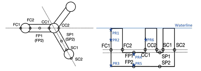
Fig. 3. Definition of the positions for hydrodynamic pressure (blue star) and stress (black circle) comparison (left: birdview; right: sideview). |
In order to compare the stress time series in the floater, several positions on the columns and the pontoons of the floater are selected and their in-plane stresses (both in the longitudinal and transverse direction of each finite element are considered for comparison, as shown as SigmaXX and SigmaYY in Fig. 5, Fig. 6, Fig. 7 and Table 5, Table 6, Table 7). As shown in Fig. 3, these ten positions are named. In particular, FP1, FP2, SP1 and SP2 are at the midpoint for the corresponding pontoons and FC1, FC2, CC1, CC2, SC1 and SC2 are located on the corresponding columns, 1 meter above the upper surface of the pontoons.
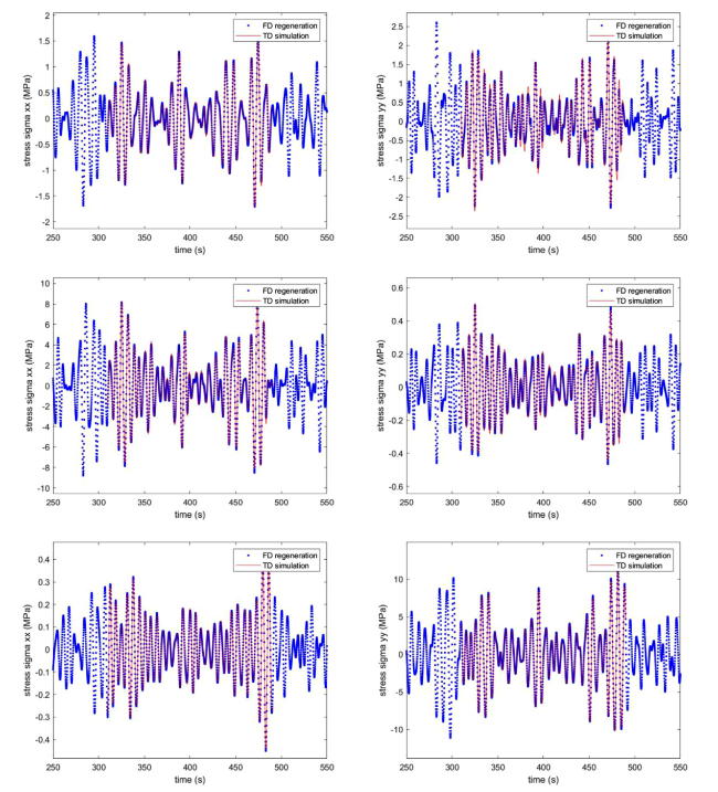
Fig. 5. Comparison of the stress times series for Case 1 by the frequency-domain regeneration (FD) and the time-domain direct analysis (TD) for the positions of FC1 (upper), FP1 (middle) and CC1 (bottom). |
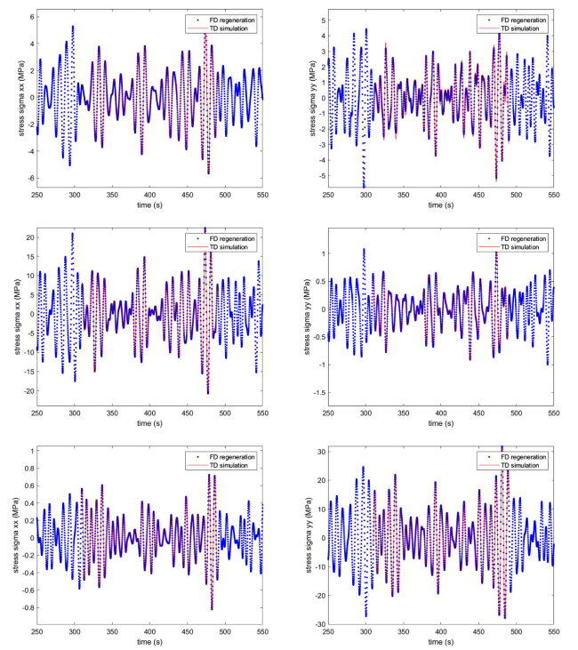
Fig. 6. Comparison of the stress times series for Case 2 by the frequency-domain regeneration (FD) and the time-domain direct analysis (TD) for the positions of FC1 (upper), FP1 (middle) and CC1 (bottom). |
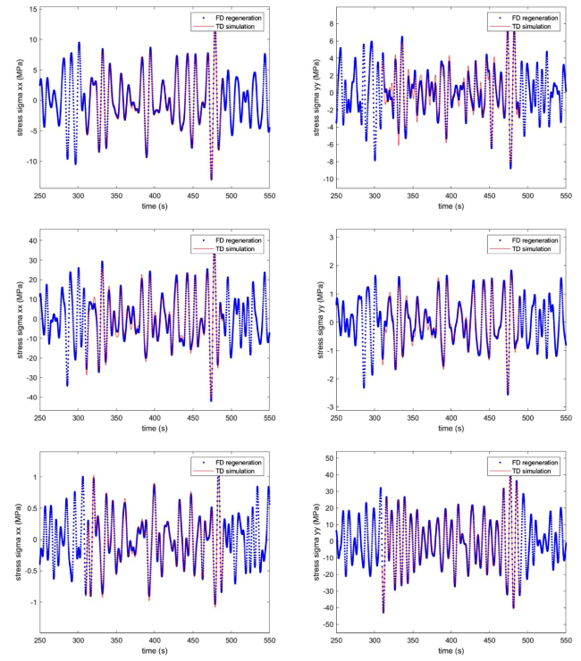
Fig. 7. Comparison of the stress times series for Case 3 by the frequency-domain regeneration (FD) and the time-domain direct analysis (TD) for the positions of FC1 (upper), FP1 (middle) and CC1 (bottom). |
Table 5. Comparison of the stress standard deviation for Case 1. |
| Case 1 | FC1 | FC2 | FP1 | FP2 | CC1 | CC2 | SC1 | SC2 | SP1 | SP2 | |
|---|---|---|---|---|---|---|---|---|---|---|---|
| Sigma_XX std | FD (MPa) | 0.56 | 0.42 | 3.01 | 2.12 | 0.14 | 0.75 | 0.25 | 0.12 | 1.34 | 0.28 |
| TD (MPa) | 0.56 | 0.41 | 2.99 | 2.10 | 0.14 | 0.74 | 0.25 | 0.12 | 1.34 | 0.29 | |
| Difference in % | −0.44% | −1.86% | −0.73% | −0.81% | −1.99% | −1.04% | −0.11% | −1.07% | −0.67% | 1.37% | |
| Sigma_YY std | FD (MPa) | 0.75 | 1.39 | 0.17 | 0.07 | 3.91 | 4.38 | 0.30 | 0.78 | 0.64 | 0.85 |
| TD (MPa) | 0.76 | 1.42 | 0.17 | 0.07 | 3.84 | 4.34 | 0.30 | 0.78 | 0.64 | 0.83 | |
| Difference in % | 1.77% | 2.19% | 0.43% | −3.76% | −1.67% | −1.02% | 2.61% | −0.57% | −0.11% | −2.12% |
Table 6. Comparison of the stress standard deviation for Case 2. |
| Case 2 | FC1 | FC2 | FP1 | FP2 | CC1 | CC2 | SC1 | SC2 | SP1 | SP2 | |
|---|---|---|---|---|---|---|---|---|---|---|---|
| Sigma_XX std | FD (MPa) | 1.95 | 1.19 | 6.67 | 4.20 | 0.26 | 1.93 | 0.74 | 0.38 | 2.61 | 0.47 |
| TD (MPa) | 1.93 | 1.19 | 6.54 | 4.11 | 0.26 | 1.91 | 0.74 | 0.38 | 2.62 | 0.48 | |
| Difference in % | −1.10% | −0.66% | −1.88% | −2.13% | −0.52% | −1.01% | −0.35% | −0.50% | 0.47% | 1.57% | |
| Sigma_YY std | FD (MPa) | 1.54 | 3.03 | 0.34 | 0.16 | 10.14 | 11.35 | 0.51 | 1.39 | 1.52 | 1.40 |
| TD (MPa) | 1.56 | 3.04 | 0.34 | 0.16 | 9.97 | 11.24 | 0.52 | 1.40 | 1.51 | 1.40 | |
| Difference in % | 1.18% | 0.43% | −1.48% | −0.05% | −1.63% | −1.01% | 2.08% | 0.19% | −0.44% | −0.06% |
Table 7. Comparison of the stress standard deviation for Case 3. |
| Case 3 | FC1 | FC2 | FP1 | FP2 | CC1 | CC2 | SC1 | SC2 | SP1 | SP2 | |
|---|---|---|---|---|---|---|---|---|---|---|---|
| Sigma_XX std | FD (MPa) | 4.40 | 3.01 | 12.99 | 8.21 | 0.41 | 3.03 | 2.02 | 1.05 | 4.04 | 1.07 |
| TD (MPa) | 4.36 | 3.01 | 12.79 | 8.08 | 0.43 | 3.00 | 2.04 | 1.07 | 4.03 | 1.20 | |
| Difference in % | −0.77% | 0.04% | −1.56% | −1.56% | 4.01% | −1.06% | 1.05% | 1.58% | −0.18% | 12.54% | |
| Sigma_YY std | FD (MPa) | 2.62 | 5.21 | 0.81 | 0.26 | 15.92 | 17.65 | 0.98 | 2.03 | 2.76 | 2.19 |
| TD (MPa) | 2.56 | 5.21 | 0.80 | 0.27 | 15.68 | 17.46 | 0.73 | 2.02 | 3.08 | 2.33 | |
| Difference in % | −2.34% | 0.05% | −1.23% | 2.70% | −1.51% | −1.05% | −24.79% | −0.57% | 11.40% | 6.45% |
5.3. Comparison of the hydrodynamic pressure components of the floater
As explained in Table 3, the dynamic components of the hydro-pressure acting on the external wet surface of the floater include the wave excitation pressure due to incident and diffracted waves, the time-varying hydrostatic pressure change (or the restoring hydrodynamic pressure) and the wave radiation pressure due to the motions of the floater. It is interesting to compare the magnitudes and the phases of these pressure components which are also dependent on the position of the floater.
In Fig. 4, the examples of the wave elevations, the floater surge, heave and pitch motions, and the hydrodynamic pressure times series are presented for Case 3 (the worst sea state considered) and for different positions of the floater. Because of the large displacement of the floater, the motions are in general quite small. Therefore, the wave radiation pressure seems to be small for all the floater positions.
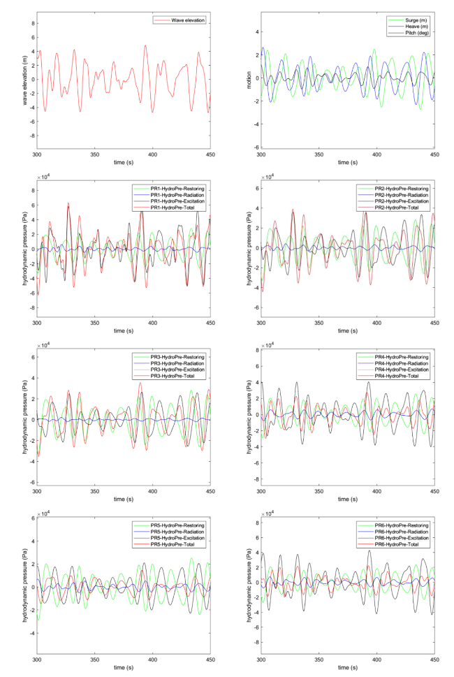
Fig. 4. Comparison of the times series for Case 3 of the wave elevation, the floater motions, the hydrodynamic pressure components at the positions of PR1-PR6. |
For the floater positions close to the waterline, the wave excitation pressure dominates, with the influence from the time-varying restoring pressure. The wave excitation pressure amplitude decreases from a position close to the waterline to a position at the column bottom, while the time-varying restoring pressure amplitude does not change since the heave motion is the same. As a result, the total hydrodynamic pressure amplitude decreases, as clearly shown in the figure.
The restoring pressure is mainly due to the heave motions and has a phase difference of 180°, while the wave excitation pressure phase angle, as compared to the wave elevation at the reference point (at the central column), depends on the horizontal distance between the position and the reference point. At the positions of PR1-PR3, the phase difference between the wave excitation pressure and the time-varying restoring pressure is close to 90°, while at PR4-PR6, it is close to 180°. This gives a very different total hydrodynamic pressure. Then the contributions from the wave radiation pressure are also important to consider.
It is important to know that the pressure considered in the comparison here only refers to the dynamic pressure. When doing the stress analysis, the time-invariant hydrostatic pressure and the gravity force, as well as the additional dynamic loads (the inertial loads, the tower bottom and the mooring line fairlead loads), should be included.
5.4. Comparison of the floater stress time series between the frequency-domain regeneration and the time-domain direct analysis
In this section, the time series of the stresses at the selected positions of FC1, FP1 and CC1 will be compared for the frequency-domain regeneration method and the time-domain simulation method, as shown in Fig. 5, Fig. 6, Fig. 7. Those positions show more significant stresses than other positions defined in Fig. 3 for the wave conditions with a direction of 0° that are considered.
For the comparison of these two methods, the same wave elevation are used as input for stress analysis, which allows to compare the stress time series directly in addition to the comparison of stress statistics. However, the frequency-domain method not only solves the stress response, but also the motion responses first, which might be slightly different when considering the resonant heave, pitch (and roll) motions as compared to the results from the time-domain approach. This is because no viscous damping is considered in the frequency-domain approach, while in the time-domain approach a linearized viscous damping is directly applied
Both the normal stresses in longitudinal and transverse directions, SigmaXX and SigmasYY, are compared. As shown in the figures, the stress time series at the different positions may have a range from 1 MPa to 20 MPa for the lowest sea state Case 1 and from 4 MPa to 80 MPa for the worst sea state Case 3. In general, the obtained stress time series from these two approaches agree very well for Case 1 and Case 2, when the waves are small or moderate. For Case 3 of the extreme waves, the differences become larger, but still very acceptable. Both methods give very similar amplitudes and phases of the stress time series, indicating all the external loads are applied correctly in the time-domain approach. For the same cases, the agreement is better for stress with significant values.
In the current study, only selected representative positions were considered for comparison. For structural design of the semi-submersible floater, one needs to identify the positions with largest stresses and perform design check.
For all the stress positions, a comparison of the statistics (standard deviation) of the stresses are given in Table 5, Table 6, Table 7. As indicated, the relative differences between the frequency-domain regeneration method and the time-domain simulation method are small, within 1-2%. However, for the Case 3, there are some observed larger differences for the stress positions of SC1, SP1 and SP2. The reason is that two different hydrodynamic analyses were performed using different frequency resolutions for the global analysis in WADAM/SIMA and for the stress transfer function analysis in WADAM/SESTRA. The WADAM model as input to SIMA has a frequency resolution of 75 frequencies for the frequency range of 0.05-3 rad/s, while the WAMIT model for pressure regeneration has 30 frequencies for the range of 0.02-3 rad/s and the WADAM model in the frequency domain approach has 60 frequencies for the range of 0.05-2.6 rad/s. This gives a slightly different transfer function of the stress around the resonant frequency of heave and pitch motions, which leads to these observed differences in stress when the waves become significant. This can be resolved by using the same frequency resolution (for example 0.05-3 rad/s with 200 frequencies) in both the frequency-domain regeneration and the time-domain simulation methods.
6. Conclusions and recommendations for future work
As part of the EMULF project, a methodology has been proposed and developed for time-domain stress analysis of a floating wind turbine floater, based on the global dynamic analysis results. The focus is to regenerate the hydrodynamic pressure load time series and apply them in a finite element model, together with other external loads from the global analysis. This methodology was illustrated using the IEA 15MW wind turbine and the UMaine semi-submersible through the developed Matlab code for hydrodynamic pressure regeneration and the DNV software packages, for wave-induced stress analysis of the floater.
Main conclusions of this study can be made as follows. The comparison of the hydrodynamic pressure components shows that both hydrodynamic pressure due to the wave excitation and time-varying restoring effects as well as their phase angles are the dominant factors for the total hydrodynamic pressure on the floater. The comparison of the floater stress time series for representative sea states shows a very good agreement between the time-domain results and the reference frequency-domain results. This indicates that the developed time-domain analysis approach can be used for engineering structural design analysis of floating wind turbines, that follows a global analysis. As compared to the traditional global analysis method, the proposed analysis procedure can directly obtain the floater stress time series that can be further used for design check. As compared to the nonlinear time domain hydrodynamic analysis code based on a Rankine-source code such as WASIM, the proposed method is more time-efficient.
The developed analysis procedure will be formally adapted by DNV in their commercial software package SESAM. The developed methodology includes a time-domain linear structural analysis using a shell-based finite element model, which is performed for each time step as in the global analysis and it is very time-consuming. Future work can include the efficient procedure for this analysis using stress influence functions for different applied loads or a pure frequency-domain stress analysis, which is currently being performed in WPE of the EMULF project. This approach can be easily extended to consider the wind induced load effects, including the tower-bottom loads and the mooring line fairlead loads. The floater motions due to the wind turbine loads and the second-order wave loads can also be easily considered for structural stress analysis, as long as the global analysis includes these effects.
It is more challenging to obtain the detailed distributions along the floater of the second-order wave pressure loads and the pressure loads due to the viscous effects and apply them for structural stress analysis. However, the magnitudes of these pressure loads are typically smaller than the first-order wave pressure loads for small and moderate seas.
As for extreme wave conditions, the nonlinear hydrodynamic analysis considering the instantaneous wet surface of the floater and the corresponding pressure may become important and should be developed for floater stress analysis as well. In such cases, a consistent hydrodynamic model for both global analysis and stress analysis should be applied. In the second phase of the EMULF project, starting from 2023.01, these aspects will be investigated.
Declaration of Competing Interests
The authors declare that they have no known competing financial interests or personal relationships that could have appeared to influence the work reported in this paper.
Acknowledgment
All the authors would like to thank COWI Fonden for the financial support through the EMULF project and the permission to publish the work in this paper.
