
1. Introduction
Countries and treaties are becoming more concerned with the sources of their energy, and to address the economic and environmental impact of our global energy system, the availability and consumption of energy resources should be considered [1]. In more recent years, targets set out by governments, treaties, and economic and political unions have brought about a resurgence in the research and development of sustainable energy technologies [2]. One of those technologies is floating photovoltaics ‘FPV’ which has proven to be a viable alternative energy source since its first installation in 2007 [3]. Since then the industry has seen substantial increases in installed capacities [4⇓-6]. Many of the installed devices have been developed for in-land waters as highlighted by Friel et al. [7], Rosa-Clot [8,9] and others. The evolution of in-land technologies to more exposed locations results in stronger demands on structural integrity, operational ability and personnel safety. A key challenge for the industry is meeting these demands whilst maintaining a low levelized cost of energy LCOE to stay cost-competitive with other sources of energy.
Existing FPV structures are typically described as floating structures that have floats which provide the hydrostatic stability for the power generating equipment and mounting structures and a mooring and anchoring system to keep the structure in position [10]. For a detailed discussion on FPV structures refer to Cazzaniga et al. [7,11], Rosa-Clot [8,9]. The structures are typically hinged, or semi-rigid structures made from polymers, steel or cementitious materials. It is understood that an appropriately designed mooring system can adjust the natural frequencies of the system out of the wave regions. A mooring system is not considered in this work, however, this work utilises a rigid support mechanism to establish an understanding of the hydrodynamic loading on a system whose natural frequencies are much greater than that of the incident wave frequencies.
Numerical and experimental methods are effective tools that can help to gain better understandings of responses and hydrodynamic effects on marine technologies. They have been extensively applied to many other applications in the marine renewable industry, for example, see Bredmose et al. [12,13] and Henderson and Zaaijer [14⇓⇓-17]. However, their application to floating solar is almost unprecedented. To date, there have been few experimental studies focused on understanding how floating solar devices perform in coastal wave climates. Borvik [18] and Winsvold [19] performed experimental investigations to determine the body kinematics and mooring line forces of toroidal shaped platforms for floating solar purposes when exposed to currents, regular and irregular waves. There have been even fewer numerical assessments of these technologies which gives rise to uncertainty in the applicability and validity of the techniques. Thus, these experiments are part of a Doctor of Philosophy Study to develop an understanding of the validity of several existing numerical codes to the application of a specific floating solar technology that utilises horizontal semi-immersed cylinders to provide the buoyancy. In Fig. 1a floating solar technology that uses horizontal cylindrical floats may be seen.
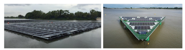
Fig. 1. (A) Floating photovoltaic system in a sheltered water body, (B) Solar duck FPV device for offshore water body. |
This study is aimed at performing an experimental investigation to:
(a) Determine the surge forces, dynamic motions and system behaviours of a scaled and simplified section of an FPV system when exposed to waves.
(b) Establish an understanding of the mechanisms and characteristics of the hydrodynamic phenomena exhibited by the structure.
(c) Obtain a dataset which can be used to aid validation and verification of numerical methods and aid system design process of a floating solar technology.
(d) Assess the magnitude of downstream wave attenuation due to the presence of the floating structure in the free surface.
The device is a horizontal cylinder type FPV system developed by SolarMarine Energy and the controlled environment is a wave flume at Queen's University Belfast. In particular, the study investigates what can be considered as the first and second cylinders within a larger array of cylinders. The model holds the assumption that it represents the first module in the array, whereby the entire structure spans many wavelengths and the first module is substantially restrained by the rest of the array. Even though the floats used in this technology are cylindrical, for which plenty of experimental data already exists when fully submerged or vertically orientated, considerable uncertainty still exists when predicting the hydrodynamic forces on the floating horizontal semi-immersed orientations. Particularly when they are close to each other. Another difficulty is present due to free-surface effects, the dynamic nature and non-linear variations in added mass, damping, drag and hydrostatic forces with changing draft.
2. Model concept
The two floating solar platforms are loosely based on the geometry and mass distribution of the gable slender technology (Fig. 3) being developed by UpSolar and SolarMarine Energy [8]. An array built of the gable slender modules is illustrated in Fig. 2. The technology utilises a catenary mooring system for station keeping. The models are referred to here as the single-cylinder model and the twin-cylinder model. The models comprise the first and second cylinders in what could be a large array of cylinders, but also may serve to aid system design of a single module system for small-scale projects.
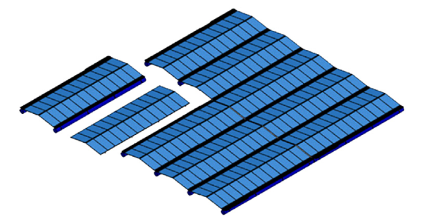
Fig. 2. Gable slender array technology. |
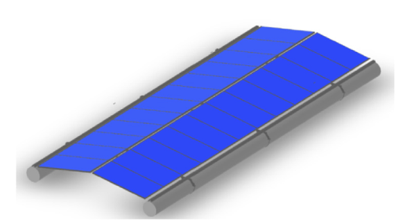
Fig. 3. Gable slender technology [8]. |
The experimental models consist of horizontal semi-immersed cylinders which provide the buoyancy. The cylinders are made of polyvinyl chloride (PVC) material and are filled with a ballasting material to provide the required draft. The floats are connected to two hollow aluminium tubes which extend further down the tank and are attached to a pin-joint mechanism that allows the aluminium members to pitch. The pin-joints are rigidly connected to two flap-plate mechanisms that contain load cells and measures the force transferred from the floats. A horizontal brace and two vertical struts are connected to the sidewall and tank base to provide the rigid-support to the models.
A Froude scaling law with a geometric scaling ratio of 1:4.54 is applied to the model for testing. In this study we consider the characteristic model length to be the diameter of the floats (0.11 m) and estimate the model-scale Froude numbers to range between 5.5 and 1.5, and Reynolds numbers ranging between 1.17e+5 and 2.20e+5 for the monochromatic sea states, this shows us that the flow state is turbulent, supercritical and inertial forces will be predominantly greater than viscous forces. There will, however, be instances where viscous forces may rise as the floats become less immersed and inversely when the floats become fully submerged. These changes in forces can introduce scaling errors when the resultant forces are transposed to the full-scale dimensions. At present there are no experimental best practices strictly applicable to floating solar technologies, however, this study has utilised the recommended practices for hydrodynamic model testing [20] (Tables 1 and 2).
Table 1. The scaled FPV model masses. |
| Component | Model scale mass (kg) | |
|---|---|---|
| Single-cylinder | Twin-cylinder | |
| Floater + ballast | 18.79 | 37.58 |
| Aluminium connecting cylinders (3m) | 1.43 | 1.43 |
| Floater connecting cylinders (1.165m) | - | 0.55 |
| Acetal adapters type 1 | 0.97 | 1.94 |
| Acetal adapters type 2 | 0.23 | 0.46 |
| U-bolts and nuts | 1.45 | 2.90 |
| Cylinder adapters type 1 | 0.41 | 0.41 |
| Cylinder adapters type 2 | - | 1.05 |
| Pin-joint mechanisms | 0.42 | 0.84 |
| Total Structural Mass | 23.70 | 47.16 |
Table 2. Experimental properties. |
| Experimental property | Dimension |
|---|---|
| Float diameter | 110.1 mm |
| Float wall thickness | 2 mm |
| Float length | 4510 mm |
| Aluminium connector diameter | 38.1 mm |
| Aluminium connector wall thickness | 1.5 mm |
| Aluminium connector length | 3000 mm |
| Float connecting cylinder length | 1165 mm |
| Displaced mass (p/cylinder) | 22.98 kg |
| Water depth | 0.765 m |
2.1. Discussion of possible error sources
Experimental models are inherently susceptible to errors and it is important to discuss these to understand the uncertainty. Kristiansen and Faltinsen [21] state that the errors may be classified as random errors, which are associated with precision, or as systematic errors. In this study, it should be noted that the precision errors related to the motion responses, load cell and wave gauge measurements were substantially low as there is good agreement between the first set of tests and the replicas. The tests were repeated once, and the results presented are the mean values. Both models span the width of the tank implying a 2-dimensional investigation, however, due to the large width of the tank, there is still the possibility of 3-dimensional hydrodynamic effects. According to equations presented by Faltinsen [22] the natural transverse sloshing periods are P1 = 0.284 s, P2 = 0.516 s,P3 = 0.685 s, and P4 = 0.813 s. The fourth is found to be in proximity of the wave excitation frequency of sea states 10 and 11. In those sea states some localised upwellings across the crests of the incident wave and some transverse wave reflections off the side panels are observed. There are also some variations in overtopping across the cylindrical floats, which may be attributed to the phenomenon. Furthermore, the cylindrical floats presence in the free surface and its motions can influence the validity of the incident wave properties due to blockage effects and reflected and radiated waves that were observed in some sea states. However, the effects appear to be less influential in the smaller amplitude waves and those with longer periods. The blockage may be quantified by considering the planar area that the submerged portion of the cylinder occupies in the water column, which is 7.2 % of the total area. There is a 0.035 m gap between the float ends and the sidewalls when the endcaps are attached to the cylinder. The spacing was sufficient to avoid contact forces between the cylinder and sidewall as no visual contacts were observed, although there were some small sway oscillations in some sea states. Moreover, there is a chance that the human operator can introduce errors when performing the experiments or when post-processing the data [22]. Additionally, should the results be transformed to full-scale dimensions then errors will be introduced which are related to viscous effects.
3. Experimental setup
Physical modelling tests are conducted in the Hydraulics Laboratory wave flume at Queen's University Belfast. The tank has a width of 4.58 m, is 18 m long, and has a maximum operating depth of 0.8 m. In Fig. 4, a top view of the twin-cylinder experimental setup is illustrated and in Fig. 5 a side view of the twin-cylinder model is illustrated. In Fig. 7 the built twin-cylinder model may be seen. The model scale ratio is 1:4.5 and is orientated such that the principal axes of the cylinders are perpendicular to the incident wave heading. This configuration is envisaged as the most critical wave heading direction which produces the largest surge loads assuming equal conditions from all directions. The aluminum beams which extend downstream are connected perpendicularly to the floats and close to the mean water level in order to help transfer the surge loading and limit vertical forces being transferred to the load measurement system. In both models, the floats and horizontal braces are rigidly connected using machined acetal adapters, whereas in the full-scale model the connections are made using steel connections. An Edinburgh Designs Ltd wave generation system is used to generate waves with discrete frequency intervals. The wavemakers are a top-hinged force feedback paddle-based system which can partially dampen reflected waves. The system has 6 paddles that move independently and can generate 3-dimensional waves; however, oblique reflections occur due to the sidewalls, therefore 2-d waves can only be generated. The side walls are panes of glass which allows for lateral observations in the water. At the end of the tank, a sloped and corrugated geotextile beach absorbs the waves.
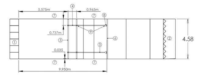
Fig. 4. Top view of twin cylinder model in wave flume. (1) Wave makers, (2) absorption beach, (3) floats, (4), aluminium connector (short), (5) aluminium connector (long), (6) horizontal brace, (7) motion capture cameras (8) hinged plate and load cell mechanism, (9) pin-joint mechanism. |

Fig. 5. Side view of twin cylinder model in wave flume. |
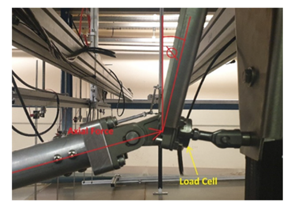
Fig. 6. Load cell and housing illustration. |
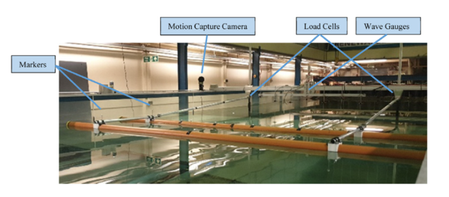
Fig. 7. Twin-cylinder experimental model and instrumentation. |
A set of heave free-decay tests were conducted on the single-cylinder model and was found to have an average natural frequency of 1.85 Hz.
Two load cells are utilised to measure the axial tension and compression forces which are transferred from the floating structure to the load cells. The load cells have an effective measurement range of 250 N and are placed to provide the surge forces that the structure undergoes. A hinged plate mechanism surrounds the devices (Fig. 6) and is designed to minimise torsional and transverse loading on the cells and are also configured such that they measure closely the horizontal force component in the loading on the device. The incident angle ∅ at which the hinged plate mechanisms are configured is 7.39°.
A Qualisys motion capture system is used in the investigation to measure the motions of several reflective markers that are attached to the floating structure. The measurement system consisted of 4 Mocap 700+ series cameras, and approximately 10 spherical reflective markers. In the twin-cylinder model, six markers are attached to some threaded dowel which raises their z-axis position 130 mm and minimises water contact. The 6 degrees of freedom are calculated in this investigation however, only the heave and pitch are of interest as the experimental model is restrained in some degrees of freedom. In Table 3 below, the results from the motion capture calibration is presented. The standard deviation of the wand length is found to be 0.6434 mm.
Table 3. Motion capture calibration. |
| Camera | X (m) | Y (m) | Z (m) | Points | Average Residual (mm) |
|---|---|---|---|---|---|
| 01 | -3.111 | -2.419 | 0.713 | 2091 | 0.713 |
| 02 | -2.323 | 2.429 | 0.719 | 1873 | 0.539 |
| 03 | 2.156 | 2.422 | 0.715 | 2090 | 0.427 |
| 04 | 2.503 | -2.417 | 0.716 | 1890 | 0.646 |
The 3-dimensional coordinates that are provided in the table represent the positions of each of the cameras concerning the global camera coordinate system. The points represent the number of computations of the distance between the global origin and each camera during calibration. The average residual is that of each of the point calculations.
The water surface elevation is measured using a total of 14 two-wire resistance-based wave probes. The wave gauge bank setup may be seen in Fig. 8. The gauges operate by measuring the resistance between a pair of parallel rods, the resistance is directly proportional to the water surface elevation. The calibration gauges are placed at the x-axis position of the centreline of the single-cylinder (x = 5.575 m), which is the same position as the first cylinder in the twin-cylinder configuration. The gauges are positioned an equal distance of 0.333 m apart in the y-axis and outwards from the y = 0 m position. The second bank of probes are situated at the x = 9.4 m location and are configured similarly. A sample rate of 128 Hz is captured from each of the sensors used in the investigation.
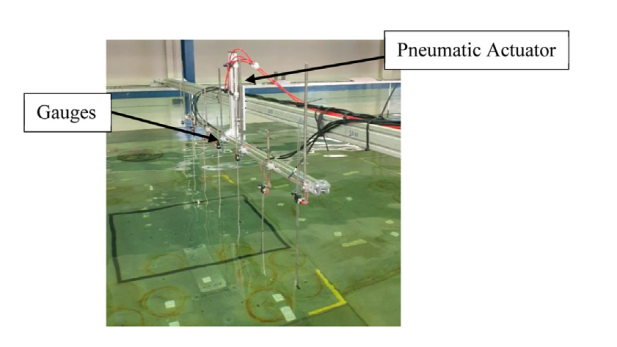
Fig. 8. Wave gauge bank setup. |
4. Environmental conditions
In this investigation, the model structure is exposed to several monochromatic and stochastic sea states. The proceeding sections discuss the environmental climates applied to the model structure, the waves have characteristic properties you may expect to find in sheltered nearshore and large lake locations. The properties are chosen to represent these locations as the device is expected to be installed in such locations. The waves at these locations have rather short periods and correspond to a location with a short fetch where locally generated wind waves are present.
4.1. Monochromatic sea states
The monochromatic sea states have a model-scale period range between 0.8 and 2 s comprising eleven sea states of various amplitudes. The calibration of the monochromatic sea states is conducted by measuring the average wave amplitude in each 128 s sea state. The recording duration includes the paddle ramp-up duration and time taken for the wave to travel to the wave probes, however the average wave amplitude is found from the steady-state region of the wave elevation time-series for each sea state. The average wave amplitude is then used in a multiplicative gain-correction factor (GCF) according to Eq. (1). The gain correction applies a modification to the tank transfer function (TTF), which relates the command voltage signals supplied to the wave-makers, to the amplitudes of the waves generated by the wave-makers.
$ \mathrm{GCF}_{\mathrm{i}}=\mathrm{GCF}_{\mathrm{i}-1} \frac{\text { Target Amplitude }}{\text { Measured Amplitude }_{\mathrm{i}}}$
It is found that each of the sea states represents an intermediate water depth and 10 out of 11 sea states may be described using a higher-order Stokes theory, with sea state 3 being described as a Cnoidal wave (Table 4).
Table 4. Monochromatic sea state properties. |
| Sea state | Model scale | Full scale | Steepness | ||||||
|---|---|---|---|---|---|---|---|---|---|
| T (s) | H/2 (m) | λ (m) | C (m/s) | T (s) | H/2 (m) | λ (m) | C (m/s) | ||
| 1 | 2.00 | 0.0282 | 4.75 | 2.38 | 4.26 | 0.144 | 21.59 | 5.06 | 0.013 |
| 2 | 2.00 | 0.0534 | 4.76 | 2.39 | 4.26 | 0.290 | 21.64 | 5.07 | 0.027 |
| 3 | 2.00 | 0.0762 | 4.79 | 2.39 | 4.26 | 0.434 | 21.77 | 5.10 | 0.040 |
| 4 | 1.33 | 0.0317 | 2.63 | 1.98 | 2.84 | 0.142 | 11.95 | 4.21 | 0.027 |
| 5 | 1.33 | 0.0502 | 2.65 | 1.98 | 2.84 | 0.296 | 12.05 | 4.24 | 0.049 |
| 6 | 1.33 | 0.0882 | 2.68 | 1.99 | 2.84 | 0.474 | 12.18 | 4.29 | 0.078 |
| 7 | 1.00 | 0.0249 | 1.57 | 1.56 | 2.13 | 0.122 | 7.14 | 3.34 | 0.034 |
| 8 | 1.00 | 0.0507 | 1.60 | 1.57 | 2.13 | 0.250 | 7.27 | 3.40 | 0.069 |
| 9 | 1.00 | 0.0781 | 1.63 | 1.59 | 2.13 | 0.448 | 7.41 | 3.48 | 0.121 |
| 10 | 0.80 | 0.0274 | 1.02 | 1.26 | 1.71 | 0.125 | 4.64 | 2.71 | 0.054 |
| 11 | 0.80 | 0.0568 | 1.07 | 1.29 | 1.71 | 0.263 | 4.86 | 2.86 | 0.108 |
4.2. Stochastic sea states
Table 5. Irregular sea state properties. |
| Sea state | Model scale | Full scale | ||
|---|---|---|---|---|
| Tp (s) | Hs (m) | Tp (s) | Hs (m) | |
| 12 | 2.00 | 0.025 | 4.26 | 0.144 |
| 13 | 2.00 | 0.050 | 4.26 | 0.290 |
| 14 | 2.00 | 0.075 | 4.26 | 0.434 |
| 15 | 1.33 | 0.030 | 2.84 | 0.142 |
| 16 | 1.33 | 0.060 | 2.84 | 0.296 |
| 17 | 1.33 | 0.075 | 2.84 | 0.474 |
| 18 | 1.00 | 0.025 | 2.13 | 0.122 |
| 19 | 1.00 | 0.050 | 2.13 | 0.250 |
| 20 | 1.00 | 0.075 | 2.13 | 0.448 |
A spectral calibration technique has been applied to ensure a specific spectral density is implemented. The method involves calculating the spectral significant wave height Hmo and mean period To1 from the 0th spectral moment. Since the magnitude of the energy at each constituent frequency is a function of the square of the wave amplitude, we use Hmo2T01 to assess the accuracy of the calibration. In addition to the above properties, we compare the area under the spectrum of the target and measured using a trapezoidal integration method and present the error εarea. The results of the spectral calibration of the irregular seas may be found in Table 5. Where Tgen is the value calculated from the realised Jonswap spectrum, M is the measured value taken from the Direct Fourier Transform (DFT) of the average measured wave-elevation, N is the number of iterations taken to achieve the respective results (Table 6).
Table 6. Spectral calibration properties. |
| Sea | N | Hmo (m) | To1 | εarea | εenergy | ||||
|---|---|---|---|---|---|---|---|---|---|
| Tgen | M | εHmo | Tgen | M | εT01 | ||||
| 12 | 2 | 0.114 | 0.114 | -0.07 | 0.572 | 0.567 | -0.75 | -0.13 | -0.88 |
| 13 | 5 | 0.228 | 0.228 | 0.83 | 0.572 | 0.572 | -0.01 | 1.65 | 1.55 |
| 14 | 2 | 0.341 | 0.341 | 0.12 | 0.572 | 0.572 | -0.21 | 0.25 | 0.04 |
| 15 | 3 | 0.137 | 0.137 | -0.23 | 0.572 | 0.390 | 0.04 | -0.47 | -0.42 |
| 16 | 2 | 0.273 | 0.273 | 0.64 | 0.390 | 0.388 | -0.61 | 1.28 | 0.69 |
| 17 | 5 | 0.337 | 0.337 | -1.93 | 0.390 | 0.397 | -1.57 | -3.89 | -2.26 |
| 18 | 3 | 0.109 | 0.109 | -0.85 | 0.303 | 0.299 | -1.32 | -1.70 | -3.05 |
| 19 | 2 | 0.223 | 0.223 | -0.03 | 0.303 | 0.294 | -2.65 | -0.06 | -2.70 |
| 20 | 2 | 0.332 | 0.332 | 2.21 | 0.303 | 0.290 | -4.63 | 4.37 | -0.05 |
5. Experimental results
In the following section experimental results, such as surge forces, motion responses and wave attenuation data are presented.
5.1. Surge forces
5.1.1. Monochromatic sea states
In Figs. 9 and 10, the normalised surge force extrema from each of the monochromatic sea states and physical models are illustrated. The extrema are plotted against the wave steepness, that is the wave height to wavelength relationship. The values presented are those taken from summing the instantaneous measurements from both load cells and then finding the maximum and minimum of the summed time-history. A linear regression line is applied to the dataset using a least-squares method. In general, the trend line reveals that there is a positive correlation in the magnitude of the surge forces as the wave steepness increases. These graphs also reveal that the twin-cylinder model generally exhibited larger surge forces than the single-cylinder model for the same sea states, and particularly more so in the sea states with larger wave steepness. Fig. 9 reveals that for both the single- and twin-cylinder models there is a strong linear positive correlation with increasing wave steepness. Whereas, Fig. 10 shows that the maxima have more variance due to the presence of outliers. To highlight the amount of variance in the surge force extrema datasets the residual sum of squares (RSS) is calculated for several wave properties. The properties include the maximum horizontal and vertical wave particle velocity, u and w, and the maximum wave particle acceleration, u˙ and w˙. These kinematic properties were calculated according to a 2nd order Stokes formulae (DNVGL-RP-C205 [20]), which is true for the majority of the monochromatic sea states. The RSS values are presented in Table 7. In general, the wave steepness shows less variance than wave height across the majority of the surge force extrema. This finding indicates that there is less uncertainty in the assumption that a linear relationship exists between wave steepness and surge force extrema, than there is with wave height and surge force extrema.
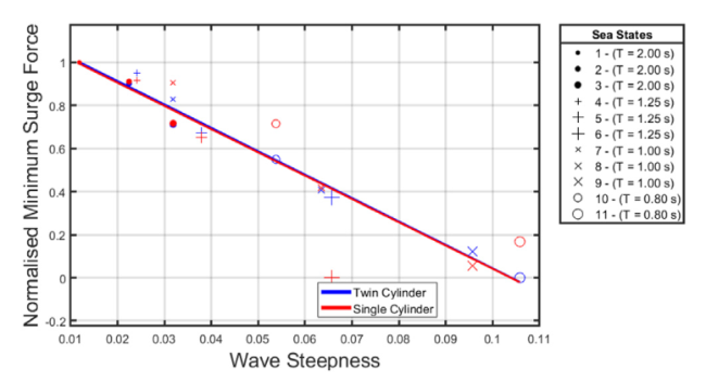
Fig. 9. Single and twin cylinder (monochromatic sea - normalised minimum surge forces). |
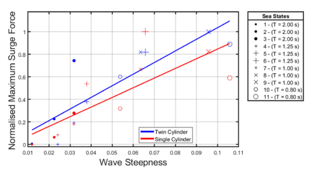
Fig. 10. Single- and twin-cylinder (monochromatic sea - normalised maximum surge forces). |
Table 7. Single cylinder - irregular sea state surge force extrema. |
| Environmental property | RSS maximum surge force | RSS minimum surge force | ||
|---|---|---|---|---|
| Twin-cylinder | Single-cylinder | Twin-cylinder | Single-cylinder | |
| Wave steepness | 21.86e+3 | 32.58e+3 | 3.57e+3 | 22.36e+3 |
| H | 38.67e+3 | 28.71e+3 | 73.78e+3 | 33.63e+3 |
| u | 12.39e+3 | 45.90e+3 | 20.81e+3 | 29.03e+3 |
| w | 13.26e+3 | 42.80e+3 | 7.45e+3 | 26.06e+3 |
| $ \dot{u} $ | 21.90e+3 | 61.26e+3 | 3.71e+3 | 46.50e+3 |
| $ \dot{ w } $ | 30.82e+3 | 64.53e+3 | 9.90e+3 | 53.26e+3 |
For the single-cylinder model sea state 6 presented the largest surge forces. The highly non-linear phenomenon known as overtopping is observed during this sea state which may have resulted in the much greater surge force measurement. The load cell measurements during the single-cylinder monochromatic sea state experiments have a good general agreement with each other, implying uniform loading across the device. The twin-cylinder model exhibited the largest forces during sea states 6, 8, 9 and 11 and the overtopping phenomenon is thought to be linked to the larger force occurrences in these sea states. The load cell measurements also had good agreement with each other except in sea state 6 where load cell two had much greater peaks than load cell one. This also occurred in sea states 5 and 11, however, the difference between the peaks of the two load cell measurements was substantially less than sea state 6.
The load cell power spectral density (PSD) for the single-cylinder model during the monochromatic sea states illustrated main peaks at the incident wave frequency and comparably small peaks at the harmonics. The load cell PSD for the twin-cylinder model had peaks at the incident wave frequency and harmonics of those frequencies. One notable twin-cylinder observation was that the 2nd harmonic of sea state 3 was approximately half the magnitude of the main peak, which can be observed in Fig. 11(a). Furthermore, this also occurred in sea states 5 and 6, The discrepancies between the two load cell readings that occurred in sea states 5 and 6 were also confirmed by the mismatch in peaks in the PSD plots, which can be observed in Fig. 11(b).
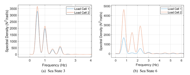
Fig. 11. Twin cylinder load cell power spectral density (Bw = Bandwidth of the Parzen window). |
5.1.2. Irregular sea states
In Table 8 below the surge force extrema recorded during the irregular sea states may be seen. The single-cylinder (SC) model exhibited the largest positive and negative surge force during sea state 20. For much of the sea states the single-cylinder model observed larger negative forces than positive. The time-history of the load cell measurements during the single- and twin-cylinder tests were found to be in good agreement with each other. A load cell time-history recorded during sea state 17 of the single- and twin-cylinder model tests may be seen in Figs. 12 and 13, respectively. One sea state where minor discrepancies were observed at the peaks and troughs was during sea state 14.
Table 8. Single cylinder - irregular sea state surge force extrema. |
| Sea state | SC - Surge force maxima (N) | SC - Surge force minima (N) | TC - Surge force maxima (N) | TC - Surge force minima (N) |
|---|---|---|---|---|
| 12 | 19.99 | -18.64 | 34.81 | -29.36 |
| 13 | 40.82 | -42.42 | 54.72 | -60.93 |
| 14 | 91.32 | -63.15 | 90.01 | -111.68 |
| 15 | 41.01 | -42.87 | 56.44 | -51.22 |
| 16 | 87.87 | -88.53 | 122.93 | -116.04 |
| 17 | 129.77 | -137.37 | 162.19 | -176.80 |
| 18 | 37.97 | -45.09 | 79.30 | -76.20 |
| 19 | 87.93 | -99.81 | 143.14 | -166.23 |
| 20 | 159.54 | -173.76 | 241.58 | -232.40 |
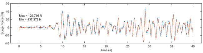
Fig. 12. Single cylinder model - load cell time-history - sea state 17. |
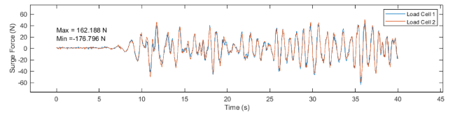
Fig. 13. Twin cylinder model - load cell time-history - sea state 17. |
In Fig. 14, the load cell spectra from the single-cylinder model tests during sea states 18-20 is illustrated. The chart presents multiple peaks throughout the various sea states which were identified as corresponding peaks in the irregular wave spectra. In Fig. 15 the load cell spectra from the twin-cylinder model tests during sea states 12-14 is shown. The twin-cylinder model spectra presented additional distinct peaks at frequencies above the peak wave frequency. The second peak in Fig. 15, Fp2, is thought to be a natural frequency of one of the modes of the structure, as it exists in all of the irregular sea state load cell spectra. In seas 15-17, the peak at this frequency is greater than the peak wave frequency and in sea states 18-20 the peak at this frequency merges with the 1 Hz peak wave frequency to form a large peak at 1.125 Hz.
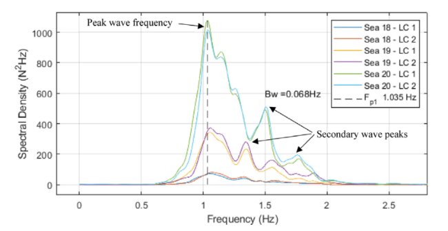
Fig. 14. Single-cylinder model - load cell spectra - sea states 18-20. |
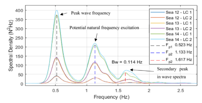
Fig. 15. Twin cylinder model - load cell spectra - sea states 12-14. |
5.2. Motion responses
5.2.1. Monochromatic sea states
One of the observations of the motion responses is a negative mean heave displacement of the structure relative to the body local origin. Both experimental models exhibited negative mean heave displacements in several sea states which means they had an average heave position lower than their natural undisturbed position throughout the wave cycles. In Fig. 16 the mean heave displacements for both models are illustrated, these values were computed as the mean of the heave motion time-history. The largest values are found to have occurred in sea states 6 and 9, and the lowest during sea states 1, 4, 7 and 10. As the latter occurred in sea states which had the lowest wave amplitudes of the applied wave frequencies, then it is safe to suggest that the wave amplitude has a strong influence on the observation, and that which is stronger than the applied range of wave frequencies. The phenomenon may be linked to greater overtopping and run-up on the floats that applies additional negative forces in the heave axis, and to the lack of hydrostatic restoring forces to counterbalance the displacement introduced by these non-linear fluid-structure interactions. As the majority of the monochromatic sea states can be described using higher-order Stokes theories, one may argue that the mean wave elevation is negatively distributed, however, the mean wave elevations are found to be no lower than -2.3 mm across all sea states.
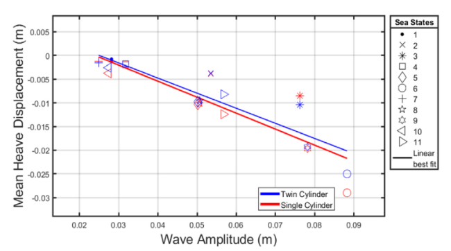
Fig. 16. Mean heave displacement monochromatic sea states. |
The time-histories and spectral densities of both models heave motions have revealed that they oscillated at the wave frequency in all sea states and a relatively small second harmonic in limited sea states. The twin-cylinder model exhibited a peculiarity in sea states 8 and 9, whereby the spectral densities shared an indistinguishable curve, although the time-histories were seen to be characteristically different. The spectral density and time-history of the aforementioned sea states may be found in Fig. 17(a) and (b), respectively. The time-histories illustrates the differences between the heave motions, the model oscillated between z = 0.0075 m and -0.0310 m in sea state 8, whereas sea states sea state 9 oscillated between z = -0.002 m and -0.042. Notably, the two shared a comparable heave displacement amplitude but around a different mean position. The comparable amplitudes have resulted in indistinguishable peaks in the spectral densities. Furthermore, in these sea states the transient event at the beginning of the time-history resulted in a low-frequency peak in both sea states, although these events were discarded for Fig. 17(a).
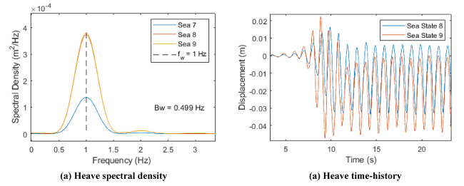
Fig. 17. Twin cylinder model heave motion results in load case 8 and 9. |
5.2.2. Irregular sea states
In Figs. 18 and 19, the heave and pitch motions of the twin-cylinder model during sea states 12 are shown respectively. The heave motion spectra of the single-cylinder model presented peaks that correspond with peaks in the incident wave spectra. The twin-cylinder heave spectral density plots of sea state 15-17 may be seen in Fig. 20. The heave motion spectra of the twin-cylinder model during all irregular sea states presented large singular peaks at the peak wave frequency. In sea states 15 and 17, however, the spectral plots reveal a large secondary peak at 1.19 Hz, and in sea state 15 a pair of peaks is situated at 1.14 and 1.32 Hz. The secondary peaks in each of these sea states are approximately half the magnitude of the peak wave frequency. In sea states 18-20, the twin-cylinder motion spectra have revealed that the peak wave frequency has merged with the peak at 1.18 Hz. The peaks occurring at 1.13-1.18 Hz may be a result of excitation at one of the model natural frequencies.
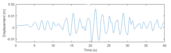
Fig. 18. Heave motions twin-cylinder model during sea state 12. |
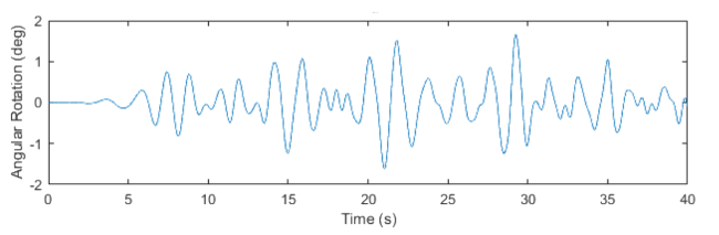
Fig. 19. Pitch motions twin-cylinder model during sea state 12. |
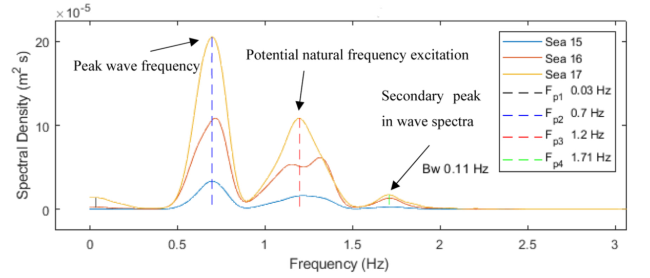
Fig. 20. Twin cylinder model heave spectral densities (sea states 15-17). |
5.3. Wave attenuation
In Fig. 21, the wave attenuation results from the monochromatic sea states may be seen. The graph illustrates the percentage change in wave amplitude between the original undisturbed wave used in calibration and the measured amplitudes during the wave climates applied to the single- and twin-cylinder models. The figure reveals that for the majority of the monochromatic sea states there is a reduction in wave amplitude due to the presence of the structure. In the lower frequency sea states, the twin-cylinder appears to have less of an effect on the reduction in amplitude than the single-cylinder. Whereas, in the higher frequency sea states the twin-cylinder model tends to attenuate the waves more than the single-cylinder model. What is striking in this chart is that there are instances where the presence of the structure acts to increase the mean measured wave amplitude, such as what is occurring in sea states 4-6.
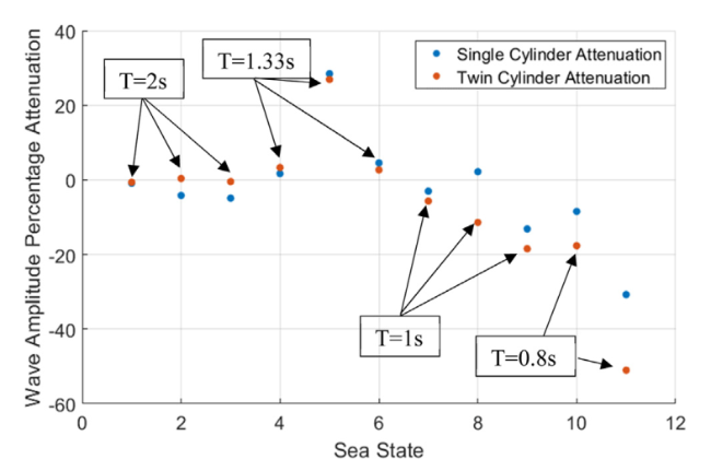
Fig. 21. Wave attenuation as a percentage change as of the original undisturbed wave amplitude. |
6. Experimental observations
6.1. Single cylinder overtopping
In several sea states, an overtopping or wave runup phenomenon has been observed. According to De Waal and Van der Meer [24], overtopping is described as the mean overtopping discharge in m3/s (volumetric flow rate), and is strongly dependent on the vertical distance between the crest of the wave and the freeboard. Other structural parameters which can influence overtopping and runup on static structures include surface roughness, model surface geometry and slope. In these experimental models, the relative motions between the float and water can also influence the phenomenon and its effects.
The phenomenon did not occur in sea states 1-5, 7, and 10. In sea states 3, 5, 10 a runup is observed however the flow of water does not pass over the cylinder, instead, the flow returns down the same face of the float. The runup on the paddle-side face of the cylinder occurs as the crest of the wave reaches the cylinder. In sea state 3 as the runup occurs, a difference in head across the front and rear sides of the cylinder is observed. This is then followed by an immediate downwards surge in fluid on the paddle-side face, and a rear-side runup as the wave crest proceeds past the centre line of the cylinder.
In Fig. 22 several examples of overtopping that occurred during the monochromatic sea states are presented. Where (a) no overtopping is observed, (b) minor overtopping is observed traversing from the paddle-side of the float, (c) a larger overtopping discharge traverses from the paddle-side of the float in one of the largest amplitude and steepest waves, and (d) an overtopping discharge or reverse flow from the beach-side is observed as the cylinder descends into the trough of the wave. In sea state 6 the floats are observed to be almost fully submerged for the entire wave cycle. The negative mean heave displacements discussed in the previous section is thought to be related to the excessive overtopping present in this sea state.

Fig. 22. Single cylinder overtopping observations. |
The phenomenon is generally observed as the crest of the wave passed the location of the cylinder. However, in one of the sea states where the most severe incidents of overtopping occurred, namely sea state 6, the cylinder begins overtopping momentarily after the trough of the wave (θ=270∘) and is submerged until the 0 degree phase angle of the wave. This finding indicates the cylinder is submerged for an estimated 75 % of the wave cycle. In Fig. 23, the single cylinder during the same sea state may be seen, the figure is separated into four sub-figures each showing the model at different phase angles of a single wave cycle. In Fig. 24, four sub-figures of another single occurrence of wave overtopping are presented.
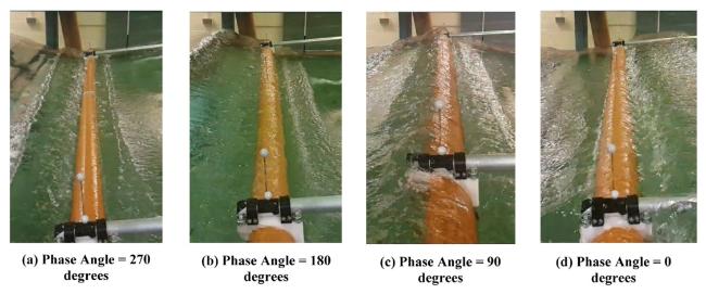
Fig. 23. Single cylinder sea state 6 - wave cycle illustration with approximate phase angles. |
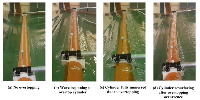
Fig. 24. Single cylinder sea state 6 - overtopping occurrence. |
Overall, these observations show that wave steepness and body position relative to the oncoming wave have an influence on the magnitude and occurrence of the overtopping wave, and potentially the global responses and loading. It is understood that the phenomenon could result in impact loading on the superstructure and photovoltaic panels, which may result in component failures.
6.2. Twin-cylinder overtopping
In several sea states, a wave runup and overtopping phenomenon are observed. The phenomenon did not occur across either cylinder in sea states 1, 2, 4, 7 and 10. During sea state 10, however some localised runup and overtopping is observed a duration into the sea, this is thought to be linked to one of the natural transverse sloshing modes occurring during the sea state. Several examples of the phenomenon have been selected and shown in Fig. 25. Where (a) a sea state where no overtopping occurs, (b) overtopping of the right-hand side cylinder may be seen, (c) moments following the image shown in (b) a dam-break spill occurs on the same cylinder and flows towards the paddles.
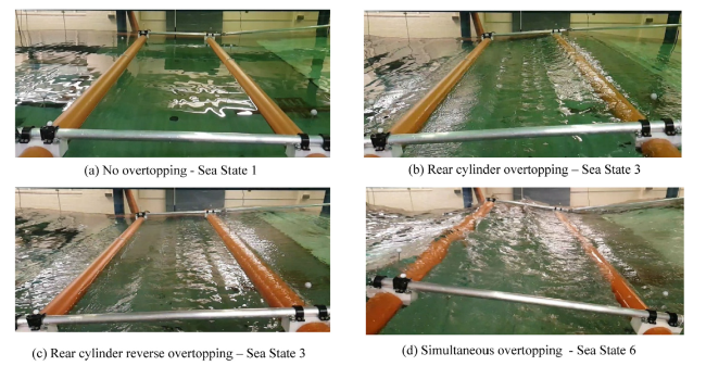
Fig. 25. Twin cylinder overtopping observation examples. |
6.3. Radiative damping and reflections
In many of the sea states and for both models the radiation damping phenomenon and reflected wave phenomena are observed. The radiative damping phenomenon occurs when the cylindrical floats descend into the trough of the wave, in turn, the float accelerates the surrounding fluid and generates a small amplitude wave that travels away from the floats in both directions. The waves generated disperse both between and away from the floats in the twin-cylinder model. The waves which are reflected towards the paddles from both cylinders tend to have a large phase celerity than those which travel towards the beach, which may be a result of the runup fluid contributing to the dispersing wave as the fluid returns towards the surface of the water body. In Fig. 26 two examples of the radiative damping phenomenon that occurred during the twin-cylinder experiments may be seen. In Fig. 27 illustrations of additional reflected and radiated waves may be seen. The internal reflections and radiated waves which occur during the irregular sea states appear to have a wide range of frequencies and amplitudes. The wave radiation between the multiple bodies in the twin-cylinder model would indicate that a numerical code that can accommodate multi-body interactions is required.
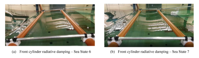
Fig. 26. Radiative damping occurrences in various sea states. |

Fig. 27. Constructive interference phenomenon between twin cylinder model during sea state 6. |
6.4. Constructive Interference
In Fig. 28, the moments leading up to and including a constructive interference occurrence is illustrated. It is believed the waves generated by the motions of each cylinder (radiative damping) combine, the incident waves and waves which occur due to overtopping which results in a vertical upwelling between the cylinders. This occurs when the waves travel towards each other and combine to cause a vertical surge of water. The phenomenon may result in impact loading on the bottom surface of the photovoltaic panels and should be considered during the design of a cylindrical type floating solar system.
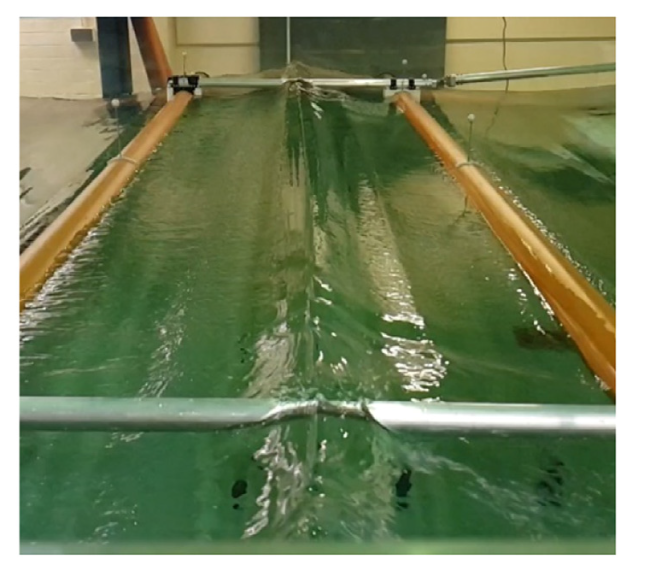
Fig. 28. Constructive interference phenomenon occurring in sea state 5. |
7. Conclusions
In this paper an experimental investigation is conducted into the wave loading, motion responses, hydrodynamic phenomena and downstream attenuation for two horizontal cylinder type rafts intended for use in a floating photovoltaic system. The investigation exposed both models to a range of monochromatic waves and irregular sea states. Surge loading measurements showed a positive correlation with wave steepness for both models in monochromatic waves. A linear regression model is applied to several wave properties and the surge force extrema of the monochromatic seas. The residual sum squared values are obtained for each and it was shown that wave steepness provided the least uncertainty in the assumption that there is a linear relationship between the two variables. In general the twin-cylinder model exhibited larger surge forces than the single-cylinder model. The largest model scale surge forces were measured during sea states 6, 9 and 11, whose values were 292.81 N, 289.05 N and -333.52 N, respectively. These values at full-scale would approximate to 27.50 kN, 27.15 kN, 31.32 kN. The hydrodynamic observations include diffraction, runup and overtopping, radiative damping and reflected waves, internal constructive interference and flow separation.
Observations of wave runup and overtopping, radiative damping and reflections indicate that these phenomena should be a design consideration of the cylindrical type floating PV system. Overtopping is a higher-order phenomenon that can result in green water effects and impact loading on a floating photovoltaic device; much of the data obtained in this study suggest that adjusting the freeboard height or draft of the floats such that the effects of overtopping be minimised. These dimensions should be designed on a site-by-site basis to reduce the likelihood of occurrence. Further investigation may be required to determine the specific short term impact loading and green water effects on the superstructure and photovoltaic panels. Furthermore, negative mean heave displacements and full-submergence of the floating cylinders implies that the superstructure and photovoltaic panels may be susceptible to impact loads due to contact with the free-surface. Future work may require that the PV panels be introduced and either force panels or pressure cells be used to accurately assess the forces (DNVGL-RP-C205 [20]).
The hydrodynamic interactions between the twin-cylinder model likely influence the loading and dynamic responses of the system, particularly in the instances where a non-linear interaction of waves between the cylinders occur. As these hydrodynamic interactions can result in additional resonance peaks and influence excitation loads it may be appropriate to apply multi-body numerical models to capture these interactions [25]. Additionally, if currents are expected at an installation site then greater considerations should be made for numerical model selection due to wake interactions between the floats.
The experimental results obtained from the model tests conducted have indicated the following key findings:
• Observations of highly non-linear fluid-structure interactions such as overtopping, constructive interference, and full float submergence during certain sea states indicate that developers should consider such effects during the design process of the floating solar technology to mitigate the negative implications they may have on the design.
• Additional peaks which are present in the surge force and heave motion spectra of the twin-cylinder model during the irregular sea states show that additional study is required to ascertain the causality of the excitation, as they may be the result of a natural frequency of one of the modes of the model test structure.
Declaration of Competing Interest
The authors declare that they have no known competing financial interests or personal relationships that could have appeared to influence the work reported in this paper.
Acknowledgments
The Bryden Centre project is supported by the European Union's INTERREG VA Programme, managed by the Special EU Programmes Body (SEUPB). The views and opinions expressed in this paper do not necessarily reflect those of the European Commission or the Special EU Programmes Body (SEUPB).
