
1. Introduction
In recent years, the diffusion-reaction equation has played an important role in dissipating dynamical systems in a variety of nonlinear sciences and engineering physics fields such as mathematical physics, chemical mathematics, ocean engineering, soliton theory, engineering science, and biological mathematics. In addition to diffusion, motion can also be due to convection. In biology, the phenomena were the main elements of a developmental process that seem to be the appearance of a traveling wave of chemical concentration. Consequently, investigations of the traveling waves play a major role in studying nonlinear convection-diffusion-reaction (NCDR) equations. Many powerful and effective methods for extracting exact analytical solutions of nonlinear evolution equations have been developed [1], [2], [3], [4], [5], [6], [8], [9], [10], [11], [12], [13], [14], [15], [16], [17], [18], [19], [20], [21], [22], [23], [24], [25], [26], [27], [28], [29], [30], [31], [32], [33], [7].
The main goal of this work is to use three efficient and systematic methods, namely the Lie symmetry analysis, the generalised Riccati equation mapping method [34], [35], [36], [37], [38], [39] and the modified Kudryashov method [40], [41] to extract multiple new solitons solutions for the NCDR equation with power law nonlinearity and density-dependent diffusion [42], [43], [44], [45], [46], which has the form
${{u}_{t}}={{\left( u\left( {{b}_{0}}+{{b}_{1}}{{u}^{p}} \right) \right)}_{x}}+{{\left( {{u}^{p+1}} \right)}_{xx}}+{{u}^{1-p}}\left( 1-{{u}^{p}} \right)\left( {{c}_{0}}+{{c}_{1}}{{u}^{p}} \right),$
in which ${{b}_{0}}$, ${{b}_{1}}$, ${{c}_{0}}$ and ${{c}_{1}}$ are real constants. More precisely, Eq. (1) is known as density-dependent diffusion for $p\ne 0$. The mentioned NCDR equation is a equation which includes the Fisher equation and various different kind of convection-diffusion-reaction equations. For$p=1$, ${{b}_{0}}={{b}_{1}}={{c}_{1}}=0$, ${{c}_{0}}=1$ NCDR equation is known as the Fisher equation or Logistic equation. When $p=1$, ${{b}_{0}}={{b}_{1}}={{c}_{0}}=0$ and ${{c}_{1}}=1$ then (1) in reduced into the Zeldovich equation. Furthermore, if $p=1$, ${{b}_{0}}={{b}_{1}}=0$ and ${{c}_{0}}={{c}_{1}}=1$, then the reduced form of NCDR equation is known as the Newell-Whitehead or amplitude equation. Eq. (1) represents the one of the certain insect dispersal models in mathematical biology [43]. It is worth mentioning here that Eq. (1) has been investigated in references [42] and [45], [46] and some new solitons and other solutions have been obtained via the simplest equation method and the extended simplest equation method, respectively.
To the best of our knowledge, Eq. (1) is not investigated via the Lie symmetry analysis, the generalized Riccati equation mapping approach, and the modified Kudryashov approach. Therefore, we must conduct our analysis and investigation to Eq. (1) to extract abundant new solitons solutions via three different techniques in a proper manner.
At the beginning of the nineteenth century, the Norwegian mathematician Sophus Lie (1842-1899) prescribed the Lie symmetry technique. Following that, Sophus Lie introduced the fundamental idea to use the invariant condition of nonlinear partial differential equations (PDEs) to obtain similarity functions and related similarity variables. This mathematical tool is highly reliable, effective, and powerful to find the exact soliton solutions of the nonlinear partial differential equations. In this technique, we first reduce the number of independent variables by one to convert the nonlinear PDEs into an ordinary differential equation (ODE). Then, we find the exact solution of the obtained ODE.
In this work, a nonlinear convection-diffusion-reaction equation (1) would be studied by employing three different mathematical methods, namely the Lie symmetry approach, the generalized Riccati equation mapping approach, and the modified Kudryashov approach. The prime objective of this work is to derive a variety of solitons and other analytical solutions to the original equation (1). Furthermore, we explore the varied dynamical wave profiles of several soliton solutions in 3D postures using numerical simulations. Nevertheless, we suggest that the evolving dynamics of the resulting soliton solutions are truly interesting and useful for complex physical phenomena.
This paper is organized as follows: Sections 2 and 3 present the Lie symmetries to the considered Eq. (1), and multiple soliton solutions are achieved. The generalized Riccati equation mapping method was retrieved and used in sections 4 and 5 to produce solitons and other solutions to the governing Eq. (1). Sections 6 and 7 describe the improved Kudryashov approach, which yields exact soliton solutions. The graphical representation of the resulting solution has been exhibited in section 8. Section 9 contains the conclusion.
2. Lie symmetry analysis
In this work, we first use the Lie symmetry analysis to construct the determining equations, infinitesimals, and vector fields for the convection-diffusion-reaction equation. For this equation, we can write the one-parameter $\left( \varepsilon \right)$ invariant transformation as
$\begin{aligned}\check{x} & \mapsto x+\varepsilon \mu_x(x, t, u)+O\left(\varepsilon^2\right), \\ \check{t} & \mapsto t+\varepsilon \mu_t(x, t, u)+O\left(\varepsilon^2\right), \\ \check{u} & \mapsto u+\varepsilon \eta(x, t, u)+O\left(\varepsilon^2\right), \end{aligned}$
where $\varepsilon $ is the group parameter and ${{\mu }_{x}}$, ${{\mu }_{t}}$ and $\eta $ represent the infinitesimal generators corresponding to x, t and u, respectively. Now, from the transformation (2), the vector field corresponding to the convection- diffusion- reaction equation has the form
$\mathbb{V}={{\mu }_{x}}\left( x,t,u \right)\frac{\partial }{\partial x}+{{\mu }_{t}}\left( x,t,u \right)\frac{\partial }{\partial t}+\eta \left( x,t,u \right)\frac{\partial }{\partial u}.$
For the existence of the Lie point symmetry of the convection-diffusion-reaction equation (1), Eq. (3) must satisfy the following condition
$P{{r}^{\left( 2 \right)}}\mathbb{V}\left( \Delta \right)=0,\ \text{whenever}\ \Delta=0\,$
where the second prolongation $P{{r}^{\left( 2 \right)}}$ corresponding to the vector field $\mathbb{V}$ can be read as
$P{{r}^{\left( 2 \right)}}\mathbb{V}=\mathbb{V}+{{\eta }^{x}}\frac{\partial }{\partial {{u}_{x}}}+{{\eta }^{t}}\frac{\partial }{\partial {{u}_{t}}}+{{\eta }^{xx}}\frac{\partial }{\partial {{u}_{xx}}}.$
Making use of $P{{r}^{\left( 2 \right)}}\mathbb{V}$ into the convection-diffusion-reaction Eq. (1), which gives the following Lie invariant surface conditions
$\begin{align} & {{\eta }^{t}}-m\left( m-1 \right)\left( {{u}^{m-2}}{{\eta }^{2x}}+{{\eta }^{-2+m}}{{u}_{x}}^{2} \right)-m\left( {{u}^{m-1}}{{\eta }^{xx}}+{{\eta }^{m-1}}{{u}_{xx}} \right) \\ & -{{b}_{0}}{{\eta }^{x}}-\left( 1+p \right){{b}_{1}}\left( {{\eta }^{p}}{{u}_{x}}+{{u}^{p}}{{\eta }^{x}} \right) \\ & -{{\eta }^{2-m}}\left( 1-{{\eta }^{p}} \right)\left( {{c}_{1}}{{\eta }^{p}}+{{c}_{0}} \right)=0, \\ \end{align}$
with coefficients
$\begin{align} & {{\eta }^{x}}={{D}_{x}}\left( \eta \right)-{{u}_{x}}{{D}_{x}}\left( {{\mu }_{x}} \right)-{{u}_{t}}{{D}_{x}}\left( {{\mu }_{t}} \right), \\ & {{\eta }^{xx}}={{D}_{x}}\left( {{\eta }^{x}} \right)-{{u}_{xx}}{{D}_{x}}\left( {{\mu }_{x}} \right)-{{u}_{xt}}{{D}_{x}}\left( {{\mu }_{t}} \right), \\ \end{align}$
and ${{D}_{x}}$ and ${{D}_{t}}$ represent the total derivative operators which can be defined as
$\begin{align} & {{D}_{x}}=\frac{\partial }{\partial x}+{{u}_{x}}\frac{\partial }{\partial u}+{{u}_{xt}}\frac{\partial }{\partial {{u}_{t}}}+{{u}_{xx}}\frac{\partial }{\partial {{u}_{x}}}\cdots, \\ & {{D}_{t}}=\frac{\partial }{\partial t}+{{u}_{t}}\frac{\partial }{\partial u}+{{u}_{xt}}\frac{\partial }{\partial {{u}_{x}}}+{{u}_{tt}}\frac{\partial }{\partial {{u}_{t}}}\cdots. \\ \end{align}$
Under the above expressions with Eq. (4) and equating the coefficients of distinct partial derivatives of u, which gives the determining equations in the following form
$\begin{align} & {{\left( {{\mu }_{x}} \right)}_{x}}=0,{{\left( {{\mu }_{x}} \right)}_{t}}=0,{{\left( {{\mu }_{x}} \right)}_{u}}=0,{{\left( {{\mu }_{t}} \right)}_{x}}=0, \\ & {{\left( {{\mu }_{t}} \right)}_{t}}=0,{{\left( {{\mu }_{t}} \right)}_{u}}=0,\eta {{\left( x,t,u \right)}_{u}}=0. \\ \end{align}$
On simplifying Eq. (5), we obtain the following infinitesimals generators
${{\mu }_{x}}={{a}_{2}},\ \ {{\mu }_{t}}={{a}_{1}},\ \ \eta =0,$
where ${{a}_{1}}$ and ${{a}_{2}}$ are free constants. The corresponding vector field $\mathbb{V}$ of the convection-diffusion-reaction equation (1) has the form
$\mathbb{V}={{a}_{1}}{{\mathbb{V}}_{1}}+{{a}_{2}}{{\mathbb{V}}_{2}},$
here ${{\mathbb{V}}_{1}}$ and ${{\mathbb{V}}_{2}}$ corresponding to ${{a}_{1}}$ and ${{a}_{2}}$ can be read as
${{\mathbb{V}}_{1}}=\frac{\partial }{\partial x},\ \ {{\mathbb{V}}_{2}}=\frac{\partial }{\partial t}.$
3. Lie symmetry reductions and soliton solutions
In this section, we utilize the Lie symmetry method to determine explicit soliton solutions of the convection-diffusion-reaction equation (1). The Lie symmetry method is one of the efficient, systematic, and straightforward mathematical tool to obtain the closed-form soliton solutions of the nonlinear evolution equations (NLEEs). Many studies have attempted to tackle a wide range of nonlinear physical problems using this technique [47], [48], [49], [50], [51], [52], [53], [54].
3.1. Subalgebra ${{\mathbb{V}}_{1}}:=\frac{\partial }{\partial x}$
The associated characteristic system can be introduced as
$\frac{dx}{1}=\frac{dt}{0}=\frac{du}{0},$
whose solution is
$u\left( x,t \right)=U\left( T \right),$
with the variable $T=t$. From Eqs. (8) and (1), we get the ordinary differential equation (ODE) as
${{c}_{0}}U\left( T \right)\left( U{{\left( T \right)}^{-p}}-1 \right)-{{c}_{1}}U\left( T \right)\left( U{{\left( T \right)}^{p}}-1 \right)-{U}'\left( T \right)=0.$
3.2. Subalgebra ${{\mathbb{V}}_{2}}:=\frac{\partial }{\partial t}$
The associated characteristic system can be introduced as
$\frac{dx}{0}=\frac{dt}{1}=\frac{du}{0},$
whose solution is
$u\left( x,t \right)=U\left( X \right),$
where U depends on X=x. Now, Eqs. (10) and (1), give the ODE of the following form
$\begin{align} & {{b}_{1}}pU{{\left( X \right)}^{p}}{U}'\left( X \right)+{U}'\left( X \right)\left( {{b}_{1}}U{{\left( X \right)}^{p}}+{{b}_{0}} \right)+\left( 1-U{{\left( X \right)}^{p}} \right)U{{\left( X \right)}^{1-p}} \\ & \left( {{c}_{1}}U{{\left( X \right)}^{p}}+{{c}_{0}} \right)+\left( p+1 \right)U{{\left( X \right)}^{p}}{U}''\left( X \right) \\ & +p\left( p+1 \right)U{{\left( X \right)}^{p-1}}{U}'{{\left( X \right)}^{2}}=0, \\ \end{align}$
whose solution can be determined a
$U\left( X \right)=\frac{\exp \left( \frac{{{c}_{0}}X}{{{b}_{0}}}+\frac{{{c}_{1}}X}{{{b}_{0}}} \right)+{{c}_{1}}\exp \left( \left( {{c}_{0}}+{{c}_{1}} \right){{k}_{1}} \right)}{\exp \left( \frac{{{c}_{0}}X}{{{b}_{0}}}+\frac{{{c}_{1}}X}{{{b}_{0}}} \right)-{{c}_{0}}\exp \left( \left( {{c}_{0}}+{{c}_{1}} \right){{k}_{1}} \right)},\ \text{provided}\ p=-1.$
Therefore, the desired solution for the NCDR equation is
$u\left( x,t \right)=\frac{\exp \left( \frac{{{c}_{0}}x}{{{b}_{0}}}+\frac{{{c}_{1}}x}{{{b}_{0}}} \right)+{{c}_{1}}\exp \left( \left( {{c}_{0}}+{{c}_{1}} \right){{k}_{1}} \right)}{\exp \left( \frac{{{c}_{0}}x}{{{b}_{0}}}+\frac{{{c}_{1}}x}{{{b}_{0}}} \right)-{{c}_{0}}\exp \left( \left( {{c}_{0}}+{{c}_{1}} \right){{k}_{1}} \right)}.$
3.3. Subalgebra ${{\mathbb{V}}_{1}}+a{{\mathbb{V}}_{2}}:=\frac{\partial }{\partial t}+a\frac{\partial }{\partial t}$
The associated characteristic system can be introduced as
$\frac{dx}{a}=\frac{dt}{1}=\frac{du}{0},$
whose solution is
$u\left( x,t \right)=U\left( X \right),$
where X=x−at. From Eq. (13) and (1), we get an ODE read as
$\begin{align} & \left( a+{{b}_{0}} \right){U}'\left( X \right)+\left( p+1 \right)U{{\left( X \right)}^{p}}\left( {{b}_{1}}{U}'\left( X \right)+{U}''\left( X \right) \right) \\ & +p\left( p+1 \right)U{{\left( X \right)}^{p-1}}{U}'{{\left( X \right)}^{2}} \\ & =U{{\left( X \right)}^{1-p}}\left( U{{\left( X \right)}^{p}}-1 \right)\left( {{c}_{1}}U{{\left( X \right)}^{p}}+{{c}_{0}} \right). \\ \end{align}$
To simplify this ODE, we use the transformation
$U\left( X \right)=G{{\left( X \right)}^{1/p}},$
which gives the ODE of the following form
$\begin{align} & {G}'\left( X \right)\left( p\left( a+{{b}_{0}} \right)+\left( p+1 \right){G}'\left( X \right) \right)+pG\left( X \right)(\left( p+1 \right)({{b}_{1}}{G}'\left( X \right) \\ & +{G}''\left( X \right))+{{c}_{1}}p)+{{c}_{1}}{{p}^{2}}\left( -G{{\left( X \right)}^{2}} \right)-{{c}_{0}}{{p}^{2}}\left( G\left( X \right)-1 \right)=0. \\ \end{align}$
Case i) For the choice of constants: $p=-1$, ${{b}_{0}}=\frac{1}{2}\left( -2a+i{{c}_{1}}{{K}_{0}}-i{{c}_{1}} \right)$, ${{c}_{0}}={{c}_{1}}-2{{c}_{1}}{{K}_{0}}$,we obtain the desired solution of ODE (16) as
$G\left( X \right)=-\frac{1}{2}i\left( {{K}_{0}}-1 \right)\tan \left( X \right)+\frac{1}{2}i\left( {{K}_{0}}-1 \right)\cot \left( X \right)+{{K}_{0}},$
where ${{K}_{0}}$ is an arbitrary constant. Therefore, the exact solution of Eq. (1) is in the form
$u\left( x,t \right)=\frac{1}{\frac{1}{2}i\left( {{K}_{0}}-1 \right)\tan \left( at-x \right)-\frac{1}{2}i\left( {{K}_{0}}-1 \right)\cot \left( at-x \right)+{{K}_{0}}}.$
Case ii) For the choice of constants: $p=-1$, ${{b}_{0}}=-a-2i{{b}_{1}}{{c}_{1}}$, ${{c}_{0}}=i\left( 4i{{b}_{1}}+i \right)c$, we get the desired solution of ODE (16) as
$G\left( X \right)=2i{{b}_{1}}\tan \left( X \right)-i\left( 2i{{b}_{1}}+i \right).$
Therefore, the exact soliton solution of Eq. (1) can be furnished as
$u\left( x,t \right)=\frac{1}{-2i{{b}_{1}}\tan \left( at-x \right)-i\left( 2i{{b}_{1}}+i \right)}.$
3.4. For ${{c}_{0}}$, ${{c}_{1}}=0$ and ${{b}_{0}}$, ${{b}_{1}}\ne 0$.
In this case, Eq. (1) is reduced into the following partial differential equation
${{u}_{t}}-{{\left( {{u}^{m}} \right)}_{xx}}-{{\left( {{b}_{1}}{{u}^{p+1}}+{{b}_{0}}u \right)}_{x}}=0,$
whose generators are
${{\mu }_{x}}=\frac{1}{2}{{a}_{3}}mx+{{a}_{5}},\ {{\mu }_{t}}={{a}_{3}}t+{{a}_{4}},\ \eta ={{a}_{3}}u,$
where ${{a}_{3}}$, ${{a}_{4}}$ and ${{a}_{5}}$ are arbitrary constants. The vectors corresponding to infinitesimal (22) can be written as
${{\mathbb{N}}_{1}}=\frac{1}{2}mx\frac{\partial }{\partial x}+t\frac{\partial }{\partial t}+u\frac{\partial }{\partial u},\ {{\mathbb{N}}_{2}}=\frac{\partial }{\partial t},\ {{\mathbb{N}}_{3}}=\frac{\partial }{\partial x}.$
3.4.1. Subalgebra ${{\mathbb{N}}_{1}}:=\frac{1}{2}mx\frac{\partial }{\partial x}+t\frac{\partial }{\partial t}+u\frac{\partial }{\partial u}$
The associated characteristic equation can be introduced as
$\frac{dx}{\frac{1}{2}mx}=\frac{dt}{t}=\frac{du}{u},$
which gives us the similarity function
$u\left( x,t \right)=tU\left( X \right),$
Where $X=x{{t}^{-\frac{m}{2}}}$. From Eqs. (23) and (1), we obtain an ODE read as
$\begin{align} & \frac{1}{2}{{t}^{-\frac{m}{2}}}{U}'\left( X \right)\left( -2{{b}_{1}}\left( p+1 \right)t{{\left( tU\left( X \right) \right)}^{p}}-2{{b}_{0}}t-mx \right)+U\left( X \right) \\ & =\frac{m{{t}^{-m}}{{\left( tU\left( X \right) \right)}^{m}}\left( \left( m-1 \right){U}'{{\left( X \right)}^{2}}+U\left( X \right){U}''\left( X \right) \right)}{U{{\left( X \right)}^{2}}}. \\ \end{align}$
3.4.2. Subalgebra ${{\mathbb{N}}_{2}}:=\frac{\partial }{\partial t}$
The associated characteristic equation gives the solution as
$u\left( x,t \right)=U\left( X \right),$
with the variable X=x. In view of Eqs. (24) and (1), we get an ODE in the following manner
$\begin{align} & U\left( X \right){U}'\left( X \right)\left( {{b}_{1}}\left( p+1 \right)U{{\left( X \right)}^{p}}+{{b}_{0}} \right) \\ & +mU{{\left( X \right)}^{m-1}}\left( \left( m-1 \right){U}'{{\left( X \right)}^{2}}+U\left( X \right){U}''\left( X \right) \right)=0. \\ \end{align}$
The exact solution of above equation for $p=1$ is
$\begin{align} & U\left( X \right)=\text{InverseFunction} \\ & \left[ -\frac{\log \left( -{{b}_{1}}{{\left( {{C}_{2}}+X \right)}^{2}}+{{b}_{0}}{{C}_{2}}+2{{C}_{1}}-X \right)-\frac{2{{b}_{0}}}{\sqrt{-8{{b}_{1}}{{C}_{1}}-b_{0}^{2}}}{{\tan }^{-1}}\left( \frac{2{{b}_{1}}\left( {{C}_{2}}+X \right)+{{b}_{0}}}{\sqrt{-8{{b}_{1}}{{C}_{1}}-b_{0}^{2}}} \right)}{{{b}_{1}}} \right], \\ \end{align}$
where ${{C}_{1}}$ and ${{C}_{2}}$ are arbitrary constants. Therefore, the desired exact solution of Eq. (1) can be furnished as
$\begin{align} & u\left( x,t \right)=\text{InverseFunction} \\ & \left[ -\frac{\log \left( -{{b}_{1}}{{\left( {{C}_{2}}+x \right)}^{2}}+{{b}_{0}}{{C}_{2}}+2{{C}_{1}}-x \right)-\frac{2{{b}_{0}}}{\sqrt{-8{{b}_{1}}{{C}_{1}}-b_{0}^{2}}}{{\tan }^{-1}}\left( \frac{2{{b}_{1}}\left( {{C}_{2}}+x \right)+{{b}_{0}}}{\sqrt{-8{{b}_{1}}{{C}_{1}}-b_{0}^{2}}} \right)}{{{b}_{1}}} \right]. \\ \end{align}$
3.4.3. Subalgebra ${{\mathbb{N}}_{2}}+\lambda {{\mathbb{N}}_{3}}:=\frac{\partial }{\partial t}+\lambda \frac{\partial }{\partial x}$
The associated characteristic system provides the similarity function
$u\left( x,t \right)=U\left( X \right),$
where $X=x-\lambda t$. In view of Eqs. (25) and (1), we get an ODE in the following manner
$\begin{align} & {U}'\left( X \right)\left( {{b}_{1}}\left( p+1 \right)U{{\left( X \right)}^{p}}+{{b}_{0}}+\lambda \right)+mU{{\left( X \right)}^{m-1}}{U}''\left( X \right) \\ & +\left( m-1 \right)mU{{\left( X \right)}^{m-2}}{U}'{{\left( X \right)}^{2}}=0. \\ \end{align}$
The solution of above ODE for $m=p=-1$ is
$U\left( X \right)=\text{InverseFunction}\left[ \frac{\left( {{b}_{0}}+\lambda \right)\log \left( {{b}_{0}}\left( {{C}_{4}}+X \right)+\lambda \left( {{C}_{4}}+X \right)+{{C}_{3}} \right)-\left( {{b}_{0}}+\lambda \right)\log \left( {{C}_{4}}+X \right)-\frac{{{C}_{3}}}{{{C}_{4}}+X}}{C_{3}^{2}} \right],$
where ${{C}_{3}}$ and ${{C}_{4}}$ are free constants. Thus, the desired exact solution of Eq. (1) is in the form
$u\left( x,t \right)=\text{InverseFunction}\left[ \frac{\left( {{b}_{0}}+\lambda \right)\log \left( {{b}_{0}}\left( {{C}_{4}}+X \right)+\lambda \left( {{C}_{4}}+X \right)+{{C}_{3}} \right)-\left( {{b}_{0}}+\lambda \right)\log \left( {{C}_{4}}+X \right)-\frac{{{C}_{3}}}{{{C}_{4}}+X}}{C_{3}^{2}} \right],$
where $X=x-\lambda t$ is similarity variable.
3.5. For ${{c}_{0}}=0$ and ${{b}_{0}}$, ${{b}_{1}}$, ${{c}_{1}}\ne 0$ in Eq. (1) with $p=m-1$.
In this case, Eq. (1) is reduced into
${{u}_{t}}-{{\left( {{u}^{m}} \right)}_{xx}}-{{\left( {{b}_{1}}{{u}^{p+1}}+{{b}_{0}}u \right)}_{x}}-{{u}^{2-m}}\left( 1-{{u}^{p}} \right)\left( {{c}_{1}}{{u}^{p}} \right)=0.$
Therefore, the corresponding vectors can be written as
$\begin{align} & {{\mathbb{M}}_{1}}=\frac{\partial }{\partial t},\ {{\mathbb{M}}_{2}}=\frac{\partial }{\partial x},\ {{\mathbb{M}}_{3}}=-{{e}^{-\left( m-1 \right){{c}_{1}}t}}{{b}_{0}}\frac{\partial }{\partial x} \\ & +{{e}^{-\left( m-1 \right){{c}_{1}}t}}\frac{\partial }{\partial t}+{{c}_{1}}{{e}^{-\left( m-1 \right){{c}_{1}}t}}u\frac{\partial }{\partial u}. \\ \end{align}$
3.5.1. Subalgebra ${{\mathbb{M}}_{2}}:=\frac{\partial }{\partial x}$
For the vector ${{\mathbb{M}}_{2}}$, we obtain
$u\left( x,t \right)=G\left( T \right),$
where T=t with m=2. Then, the convection-diffusion-reaction equation converts into the ODE
${{c}_{1}}\left( -\left( G\left( T \right)-1 \right) \right)G\left( T \right)-{G}'\left( T \right)=0,$
whose solution is
$G\left( T \right)=\frac{{{e}^{{{c}_{1}}T}}}{{{e}^{{{c}_{1}}T}}+{{e}^{{{K}_{1}}}}},$
where ${{K}_{1}}$ is an arbitrary constant. Therefore, Eq. (1) has the following exact solution
$u\left( x,t \right)=\frac{{{e}^{{{c}_{1}}t}}}{{{e}^{{{c}_{1}}t}}+{{e}^{{{K}_{1}}}}}.$
3.5.2. Subalgebra ${{\mathbb{M}}_{3}}:=-{{e}^{-\left( m-1 \right){{c}_{1}}t}}{{b}_{0}}\frac{\partial }{\partial x}+{{e}^{-\left( m-1 \right){{c}_{1}}t}}\frac{\partial }{\partial t}+{{c}_{1}}{{e}^{-\left( m-1 \right){{c}_{1}}t}}u\frac{\partial }{\partial u}$
The associated characteristic system can be introduced as
$\frac{dx}{-{{b}_{0}}{{e}^{-\left( m-1 \right){{c}_{1}}t}}}=\frac{dt}{{{e}^{-\left( m-1 \right){{c}_{1}}t}}}=\frac{du}{{{c}_{1}}{{e}^{-\left( m-1 \right){{c}_{1}}t}}u},$
whose solution is
$u\left( x,t \right)=\exp \left( {{c}_{1}}t \right)G\left( X \right),$
where $X=x+{{b}_{0}}t$. From Eqs. (34) and (1), we get an ODE in the following manner
$\frac{{{\left( {{e}^{{{c}_{1}}t}}G\left( X \right) \right)}^{m}}\left( mG\left( X \right)\left( {{b}_{1}}{G}'\left( X \right)+{G}''\left( X \right) \right)-{{c}_{1}}G{{\left( X \right)}^{2}}+\left( m-1 \right)m{G}'{{\left( X \right)}^{2}} \right)}{G{{\left( X \right)}^{2}}}=0.$
On simplifying above equation, we obtain exact solition solutions as
$G\left( X \right)={{K}_{3}}\exp \left( -\frac{{{b}_{1}}X-2\log \left( \cos \left( \frac{1}{2}X\sqrt{-b_{1}^{2}-4{{c}_{1}}}-\frac{1}{2}{{K}_{2}}m\sqrt{-b_{1}^{2}-4{{c}_{1}}} \right) \right)}{2m} \right),$
$\begin{align} & G\left( X \right)=\left( {{b}_{0}}+4i \right)\tan \left( X \right)+\left( -{{b}_{0}}-4i \right)\cot \left( X \right)-2i\left( {{b}_{0}}+4i \right), \\ & \text{provided}\ m=-1,{{b}_{1}}=4i,{{c}_{1}}=0, \\ \end{align}$
$G\left( X \right)=\frac{i\tan \left( X \right)}{{{b}_{0}}-2i}-\frac{1}{{{b}_{0}}-2i},\ \text{provided}\ m=-1,{{b}_{1}}=-2i,{{c}_{1}}=0,$
$G\left( X \right)=\frac{\tan \left( X \right)}{{{b}_{0}}+2i}+\frac{\cot \left( X \right)}{{{b}_{0}}+2i},\ \text{provided}\ m=-1,{{b}_{1}}=0,{{c}_{1}}=-4,$
where ${{K}_{2}}$ and ${{K}_{3}}$ are arbitrary constant. Thus, from (34) and (35), (36), (37), (38), we deduce the following solutions of Eq. (1) as
$u\left( x,t \right)={{K}_{3}}\exp \left( {{c}_{1}}t-\frac{{{b}_{1}}\left( {{b}_{0}}t+x \right)-2\log \left( \cos \left( \frac{1}{2}\sqrt{-b_{1}^{2}-4{{c}_{1}}}\left( {{b}_{0}}t+x \right)-\frac{1}{2}{{K}_{2}}m\sqrt{-b_{1}^{2}-4{{c}_{1}}} \right) \right)}{2m} \right),$
$u\left( x,t \right)=\frac{i\tan \left( {{b}_{0}}t+x \right)}{{{b}_{0}}-2i}-\frac{1}{{{b}_{0}}-2i},$
$u\left( x,t \right)=\left( {{b}_{0}}+4i \right)\tan \left( {{b}_{0}}t+x \right)\left( -{{\left( \cot \left( {{b}_{0}}t+x \right)+i \right)}^{2}} \right),$
$u\left( x,t \right)={{e}^{-4t}}\left( \frac{\tan \left( {{b}_{0}}t+x \right)}{{{b}_{0}}+2i}+\frac{\cot \left( {{b}_{0}}t+x \right)}{{{b}_{0}}+2i} \right).$
3.6. For ${{c}_{0}}=0$, ${{c}_{1}}=0$, ${{b}_{1}}=0$ and ${{b}_{0}}\ne 0$ in Eq. (1).
In this case, Eq. (1) is reduced into the partial differential equation of the following form
${{u}_{t}}-{{\left( {{u}^{m}} \right)}_{xx}}-{{\left( {{b}_{0}}u \right)}_{x}}=0,$
whose infinitesimal generators are
${{\mu }_{x}}=\frac{1}{2}{{a}_{6}}mx+{{a}_{8}},{{\mu }_{t}}={{a}_{6}}t+{{a}_{7}},\eta ={{a}_{6}}u,$
where ${{a}_{6}}$, ${{a}_{7}}$ and ${{a}_{8}}$ are arbitrary constants. From the infinitesimal generators, we obtain vectors of the following form
${{\mathbb{P}}_{1}}=\frac{1}{2}mx\frac{\partial }{\partial x}+t\frac{\partial }{\partial t}+u\frac{\partial }{\partial u},\ {{V}_{10}}=\frac{\partial }{\partial t},\ {{\mathbb{P}}_{3}}=\frac{\partial }{\partial x}.$
3.6.1. Subalgebra ${{\mathbb{P}}_{2}}:=\frac{\partial }{\partial t}$
The associated characteristic equation gives the solution as
$u\left( x,t \right)=U\left( X \right),$
with the variable X=x. In view of Eqs. (45) and (1), we get an ODE in the following manner
${{b}_{0}}{U}'\left( x \right)+mU{{\left( x \right)}^{m-2}}\left( \left( m-1 \right){U}'{{\left( x \right)}^{2}}+U\left( x \right){U}''\left( x \right) \right)=0.$
The desired exact product log solution of above equation is
$U\left( X \right)=\frac{2{{K}_{4}}W\left( -\frac{1}{2{{K}_{4}}}\exp \left( -\frac{b_{0}^{2}\left( {{K}_{5}}+X \right)}{4{{K}_{4}}}-1 \right) \right)}{{{b}_{0}}}+\frac{2{{K}_{4}}}{{{b}_{0}}}.$
Thus, we get
$u\left( x,t \right)=\frac{2{{K}_{4}}W\left( -\frac{1}{2{{K}_{4}}}\exp \left( -\frac{b_{0}^{2}\left( {{K}_{5}}+x \right)}{4{{K}_{4}}}-1 \right) \right)}{{{b}_{0}}}+\frac{2{{K}_{4}}}{{{b}_{0}}},$
where ${{K}_{4}}$ and ${{K}_{5}}$ are arbitrary constants.
3.6.2. Subalgebra ${{\mathbb{P}}_{2}}+\lambda {{\mathbb{P}}_{3}}:=\frac{\partial }{\partial t}+\lambda \frac{\partial }{\partial x}$
The associated characteristic equation provides the solution
$u\left( x,t \right)=U\left( X \right),$
where $X=x-\lambda t$. In view of Eqs. (48) and (1), we get an ODE in the following manner
$\left( {{b}_{0}}+\lambda \right){U}'\left( X \right)+mU{{\left( X \right)}^{m-1}}{U}''\left( X \right)+\left( m-1 \right)mU{{\left( X \right)}^{m-2}}{U}'{{\left( X \right)}^{2}}=0.$
Thus, the desired solution of above ODE is
$U\left( X \right)=\frac{2{{K}_{6}}\left( W\left( \frac{1}{2{{K}_{6}}}\exp \left( -\frac{{{b}_{0}}\left( {{b}_{0}}+2\lambda \right)\left( {{K}_{7}}+X \right)+{{\lambda }^{2}}\left( {{K}_{7}}+X \right)+4{{K}_{6}}}{4{{K}_{6}}} \right) \right)+1 \right)}{{{b}_{0}}+\lambda },\text{provided}\ m=2.$
Therefore, the solution of equation (1) is in the form
$u\left( x,t \right)=\frac{2{{K}_{6}}\left( W\left( \frac{1}{2{{K}_{6}}}\exp \left( -\frac{{{b}_{0}}\left( {{b}_{0}}+2\lambda \right)\left( {{K}_{7}}-\lambda t+x \right)+{{\lambda }^{2}}\left( {{K}_{7}}-\lambda t+x \right)+4{{K}_{6}}}{4{{K}_{6}}} \right) \right)+1 \right)}{{{b}_{0}}+\lambda }.$
4. A generalized riccati equation mapping method overview
Step 1. Consider a PDE of nonlinear type in two independent variables x, t and one dependent variable $\Gamma$ in the form
$Q\left( \Gamma,{{\Gamma}_{x}},{{\Gamma}_{t}},{{\Gamma}_{xx}},{{\Gamma}_{xt}},{{\Gamma}_{tt}},\cdots \right)=0,$
in which Q represent a polynomial in $\Gamma\left( x,t \right)$ and corresponding partial derivatives provided both of the highest order derivatives and nonlinear terms are existed.
Step 2. Let us assume the following ansatz transformation
$\Gamma\left( x,t \right)=\Gamma\left( \eta \right),\ \ \ \eta =x-{{\Omega}_{1}}t,$
where ${{\Omega}_{1}}$ is the speed wave constant. By (53), we can reduce Eq. (52) to the nonlinear ODE
$S\left( \Gamma\left( \eta \right),{{\Gamma}^{\prime }}\left( \eta \right),{{\Gamma}^{\prime\prime }}\left( \eta \right),\cdots \right)=0,$
where S represents a polynomial in $\Gamma\left( \eta \right)$ and its derivatives with respect to the variable $\eta $.
Step 3. Assume that Eq. (54) has the formal form of the solution as
$\Gamma\left( \eta \right)=\underset{k=0}{\overset{Z}{\mathop \sum }}\,{{A}_{k}}{{W}^{k}}\left( \eta \right),$
where ${{A}_{k}}\ \left( k=0,1,2,\cdots,Z \right)$ are undetermined constants, Z is a positive integer that should be determined via balancing principle between the highest order derivative term and the highest power nonlinear terms in Eq. (54), while $W\left( \eta \right)$ satisfies the constant coefficients generalized Riccati equation
${W}'\left( \eta \right)={{w}_{0}}+{{w}_{1}}W\left( \eta \right)+{{w}_{2}}{{W}^{2}}\left( \eta \right),$
where ${W}'=\frac{dW}{d\eta }$ and ${{w}_{0}}$, ${{w}_{1}}$ and ${{w}_{2}}$ are arbitrary constants such that ${{w}_{2}}\ne 0$.
${{W}_{+}}\left( \eta \right)=-\frac{\sqrt{\Sigma}\left( {{\lambda }_{1}}\tanh \left( \frac{\eta \sqrt{\Sigma}}{2} \right)+{{\lambda }_{2}} \right)}{\left( 2{{w}_{2}} \right)\left( {{\lambda }_{2}}\tanh \left( \frac{\eta \sqrt{\Sigma}}{2} \right)+{{\lambda }_{1}} \right)}-\frac{{{w}_{1}}}{2{{w}_{2}}},\Sigma>0,\lambda _{1}^{2}+\lambda _{2}^{2}\ne 0,$
${{W}_{-}}\left( \eta \right)=\frac{\sqrt{-\Sigma}\left( {{\lambda }_{3}}\tan \left( \frac{\eta \sqrt{-\Sigma}}{2} \right)-{{\lambda }_{4}} \right)}{\left( 2{{w}_{2}} \right)\left( {{\lambda }_{4}}\tan \left( \frac{\eta \sqrt{-\Sigma}}{2} \right)+{{\lambda }_{3}} \right)}-\frac{{{w}_{1}}}{2{{w}_{2}}},\Sigma0,\lambda _{3}^{2}+\lambda _{4}^{2}\ne 0,$
${{W}_{0}}\left( \eta \right)=-\frac{1}{\eta {{w}_{2}}+w}-\frac{{{w}_{1}}}{2{{w}_{2}}},\ \Sigma=0,$
$W\left( \eta \right)=\frac{\frac{\epsilon \sqrt{\Sigma\left( {{F}^{2}}+{{G}^{2}} \right)}\text{sech}\left( \eta \sqrt{\Sigma} \right)-F\sqrt{\Sigma}}{F\tanh \left( \eta \sqrt{\Sigma} \right)+G\text{sech}\left( \eta \sqrt{\Sigma} \right)}-{{w}_{1}}}{2{{w}_{2}}},$
$W\left( \eta \right)=\frac{-\frac{\epsilon \sqrt{\Sigma\left( {{F}^{2}}+{{G}^{2}} \right)}\text{sech}\left( \eta \sqrt{\Sigma} \right)+F\sqrt{\Sigma}}{F\tanh \left( \eta \sqrt{\Sigma} \right)+G\text{sech}\left( \eta \sqrt{\Sigma} \right)}-{{w}_{1}}}{2{{w}_{2}}},$
$W\left( \eta \right)=\frac{\frac{\epsilon \sqrt{\Sigma\left( -\left( {{F}^{2}}-{{G}^{2}} \right) \right)}\sec \left( \eta \sqrt{-\Sigma} \right)-F\sqrt{-\Sigma}}{F\tan \left( \eta \sqrt{-\Sigma} \right)+G\sec \left( \eta \sqrt{-\Sigma} \right)}-{{w}_{1}}}{2{{w}_{2}}},$
$W\left( \eta \right)=\frac{-\frac{\epsilon \sqrt{\Sigma\left( -\left( {{F}^{2}}-{{G}^{2}} \right) \right)}\sec \left( \eta \sqrt{-\Sigma} \right)+F\sqrt{-\Sigma}}{F\tan \left( \eta \sqrt{-\Sigma} \right)+G\sec \left( \eta \sqrt{-\Sigma} \right)}-{{w}_{1}}}{2{{w}_{2}}},$
where ${{\lambda }_{r}}$ for r=1,2,3,4 are arbitrary constants, w is an integrating constant and $\Sigma=w_{1}^{2}-4{{w}_{0}}{{w}_{2}}$.
Step 5. Substituting (55) into Eq. (54) and using (56) with collection of all the coefficients of ${{W}^{k}}\left( \eta \right)\ \left( k=0,1,2,\ldots,Z \right)$ and setting them to zero, we get a system of nonlinear algebraic equations for ${{A}_{k}}\ \left( k=0,1,2,\ldots,Z \right)$, ${{w}_{0}}$, ${{w}_{1}}$, ${{w}_{2}}$ and ${{\Omega}_{1}}$.
Step 6. On solving the system of these nonlinear algebraic equations and using the solutions (57)-(63) of Eq. (56), we can obtain the solutions of the original Eq. (1).
Now, we will solve Eq. (1) via the generalized Riccati equation mapping method as in the following section.
5. Soliton solutions of NCDR (1) via the generalized riccati equation mapping method
Making the transformation
$u\left( x,t \right)=Q\left( \eta \right),\ \ \ \eta =x-{{\Omega}_{1}}t,$
so that Eq. (1) is reduced to the ODE
$\begin{align} & -\left( {{b}_{0}}-{{\Omega}_{1}} \right){Q}'\left( \eta \right){{Q}^{-p}}\left( \eta \right)+{{b}_{1}}\left( p+1 \right){Q}'\left( \eta \right) \\ & +p\left( p+1 \right){{Q}^{-1}}\left( \eta \right){{{{Q}'}}^{2}}\left( \eta \right)+\left( p+1 \right){Q}''\left( \eta \right)+{{c}_{0}}{{Q}^{1-2p}}\left( \eta \right) \\ & +\left( {{c}_{1}}-{{c}_{0}} \right){{Q}^{1-p}}\left( \eta \right)-{{c}_{1}}Q\left( \eta \right)=0. \\ \end{align}$
Balancing ${Q}''\left( \eta \right)$ and ${Q}'\left( \eta \right){{Q}^{-p}}\left( \eta \right)$ to obtain $Z=-\frac{1}{p}$. Using the transformation
$Q\left( \eta \right)={{\Gamma}^{-\frac{1}{p}}}\left( \eta \right),$
then Eq. (65) is reduced to the following nonlinear ODE
$\begin{align} & -p\left( {{b}_{0}}+{{\Omega}_{1}} \right)\Gamma{{\left( \eta \right)}^{2}}{{\Gamma}^{\prime }}\left( \eta \right)-{{b}_{1}}p\left( p+1 \right)\Gamma\left( \eta \right){{\Gamma}^{\prime }}\left( \eta \right) \\ & +{{c}_{0}}{{p}^{2}}\Gamma{{\left( \eta \right)}^{4}}+\left( {{c}_{1}}-{{c}_{0}} \right){{p}^{2}}\Gamma{{\left( \eta \right)}^{3}}-{{c}_{1}}{{p}^{2}}\Gamma{{\left( \eta \right)}^{2}} \\ & +\left( 2{{p}^{2}}+3p+1 \right){{\Gamma}^{\prime }}{{\left( \eta \right)}^{2}}-p\left( p+1 \right)\Gamma\left( \eta \right){{\Gamma}^{\prime\prime }}\left( \eta \right)=0. \\ \end{align}$
Balancing $\Gamma{{\Gamma}^{\prime\prime }}$ as the highest order derivative term with ${{\Gamma}^{4}}$ as the highest power nonlinear term, we get $Z=1$. As a consequence, Eq. (67) admits the formal solution
$\Gamma\left( \eta \right)={{A}_{0}}+{{A}_{1}}W\left( \eta \right),$
where ${{A}_{k}}\ \left( k=0,1 \right)$ are undetermined constants. Substituting (68) into (67) and using (68) with equating the coefficients of ${{W}^{k}}\left( \eta \right)\ \left( k=0,1,2,\ldots,5 \right)$ to zero, yield a system of nonlinear algebraic equations for the unknown ${{A}_{k}},{{w}_{l}}\ \left( k=0,1;l=0,1,2 \right)$ and ${{\Omega}_{1}}$.
Solving this system of resultant algebraic equations via Mathematica symbolic computations, we thus obtain the following results
$\begin{align} & \mathbf{Output1}.{{A}_{0}}=0,{{A}_{1}}={{A}_{1}},\ {{w}_{0}}=0,{{w}_{1}}={{w}_{1}},{{w}_{2}}=-{{A}_{1}}{{w}_{1}}, \\ & {{c}_{1}}=\frac{\left( p+1 \right){{w}_{1}}\left( \left( p+1 \right){{w}_{1}}-{{b}_{1}}p \right)}{{{p}^{2}}}, \\ & {{\Omega}_{1}}=\frac{2{{w}_{2}}}{{{A}_{1}}p}-{{b}_{0}}-\frac{{{c}_{0}}p}{{{w}_{1}}}+\left( \frac{1}{p}-1 \right){{w}_{1}}, \\ \end{align}$
$\begin{align} & \mathbf{Output}\ \mathbf{2}.{{A}_{0}}=0,{{A}_{1}}={{A}_{1}},\ {{w}_{0}}=0,{{w}_{1}}={{w}_{1}},{{w}_{2}}={{w}_{2}}, \\ & {{c}_{0}}=-\frac{{{w}_{2}}\left( p+1 \right)\left( {{b}_{1}}p-{{w}_{1}}\left( p+1 \right) \right)}{{{A}_{1}}{{p}^{2}}}, \\ & {{c}_{1}}=\frac{{{A}_{1}}{{c}_{0}}{{w}_{1}}}{{{w}_{2}}},{{\Omega}_{1}}=\frac{{{A}_{1}}{{c}_{0}}p}{{{w}_{2}}}+\frac{{{w}_{2}}\left( p+1 \right)}{{{A}_{1}}p}-{{b}_{0}}, \\ \end{align}$
$\begin{align} & \mathbf{Output}\ \mathbf{3}.{{A}_{0}}=0,{{A}_{1}}={{A}_{1}},\ {{w}_{0}}=0,{{w}_{1}}={{w}_{1}},{{w}_{2}}={{A}_{1}}{{w}_{1}}, \\ & {{c}_{1}}=\frac{\left( p+1 \right){{w}_{1}}\left( \left( p+1 \right){{w}_{1}}-{{b}_{1}}p \right)}{{{p}^{2}}},{{c}_{0}}={{c}_{1}}, \\ & {{\Omega}_{1}}=\frac{\left( p+1 \right)\left( p+2 \right){{w}_{1}}-p\left( {{b}_{1}}\left( p+1 \right)+{{b}_{0}} \right)}{p}. \\ \end{align}$
Substituting (69) with (57), (58) and (60)-(63) into (68) and using (64) yields the traveling wave solutions of Eq. (1) in the form
$u\left( x,t \right)={{\left\{ \frac{1}{2}\left( 1+\frac{{{\lambda }_{1}}\tanh \left( \frac{p\left( \epsilon \sqrt{b_{1}^{2}+4{{c}_{1}}}+{{b}_{1}} \right)}{4\left( p+1 \right)}\eta \right)+{{\lambda }_{2}}}{{{\lambda }_{2}}\tanh \left( \frac{p\left( \epsilon \sqrt{b_{1}^{2}+4{{c}_{1}}}+{{b}_{1}} \right)}{4\left( p+1 \right)}\eta \right)+{{\lambda }_{1}}} \right) \right\}}^{-\frac{1}{p}}},$
provided $b_{1}^{2}+4{{c}_{1}}>0\ \epsilon =\pm 1$, and $\eta =x-t\left( -\frac{2{{c}_{0}}\left( p+1 \right)}{\epsilon \sqrt{b_{1}^{2}+4{{c}_{1}}}+{{b}_{1}}}-\frac{1}{2}\left( \epsilon \sqrt{b_{1}^{2}+4{{c}_{1}}}+{{b}_{1}} \right)-{{b}_{0}} \right).$
$u\left( x,t \right)={{\left\{ \frac{1}{2}\left( 1-\frac{i\left( {{\lambda }_{3}}\tan \left( \frac{ip\left( \epsilon \sqrt{b_{1}^{2}+4{{c}_{1}}}+{{b}_{1}} \right)}{4\left( p+1 \right)}\eta \right)-{{\lambda }_{4}} \right)}{{{\lambda }_{4}}\tan \left( \frac{p\left( \epsilon \sqrt{b_{1}^{2}+4{{c}_{1}}}+{{b}_{1}} \right)}{4\left( p+1 \right)}\eta \right)+{{\lambda }_{3}}} \right) \right\}}^{-\frac{1}{p}}},$
provided $b_{1}^{2}+4{{c}_{1}}>0$, $i=\sqrt{-1}$ and $\epsilon =\pm 1$, where $\eta =x-t\left( -\frac{2{{c}_{0}}\left( p+1 \right)}{\epsilon \sqrt{b_{1}^{2}+4{{c}_{1}}}+{{b}_{1}}}-\frac{1}{2}\left( \epsilon \sqrt{b_{1}^{2}+4{{c}_{1}}}+{{b}_{1}} \right)-{{b}_{0}} \right),$
$u\left( x,t \right)={{\left\{ \frac{1}{2}\left( 1-\frac{\sqrt{{{F}^{2}}+{{G}^{2}}}\text{sech}\left( \frac{p\left( \epsilon \sqrt{b_{1}^{2}+4{{c}_{1}}}+{{b}_{1}} \right)}{2\left( p+1 \right)}\eta \right)-F}{F\tanh \left( \frac{p\left( \epsilon \sqrt{b_{1}^{2}+4{{c}_{1}}}+{{b}_{1}} \right)}{2\left( p+1 \right)}\eta \right)+G\text{sech}\left( \frac{p\left( \epsilon \sqrt{b_{1}^{2}+4{{c}_{1}}}+{{b}_{1}} \right)}{2\left( p+1 \right)}\eta \right)} \right) \right\}}^{-\frac{1}{p}}},$
provided $b_{1}^{2}+4{{c}_{1}}>0$, ${{F}^{2}}+{{G}^{2}}>0$ and $\epsilon =\pm 1$ where $\eta =x-t\left( -\frac{2{{c}_{0}}\left( p+1 \right)}{\epsilon \sqrt{b_{1}^{2}+4{{c}_{1}}}+{{b}_{1}}}-\frac{1}{2}\left( \epsilon \sqrt{b_{1}^{2}+4{{c}_{1}}}+{{b}_{1}} \right)-{{b}_{0}} \right),$
$u\left( x,t \right)={{\left\{ \frac{1}{2}\left[ 1-i\left( \frac{\sqrt{{{F}^{2}}-{{G}^{2}}}\sec \left( \frac{ip\left( \epsilon \sqrt{b_{1}^{2}+4{{c}_{1}}}+{{b}_{1}} \right)}{2\left( p+1 \right)}\eta \right)-F}{F\tan \left( \frac{ip\left( \epsilon \sqrt{b_{1}^{2}+4{{c}_{1}}}+{{b}_{1}} \right)}{2\left( p+1 \right)}\eta \right)+G\sec \left( \frac{ip\left( \epsilon \sqrt{b_{1}^{2}+4{{c}_{1}}}+{{b}_{1}} \right)}{2\left( p+1 \right)}\eta \right)} \right) \right] \right\}}^{-\frac{1}{p}}},$
provided $b_{1}^{2}+4{{c}_{1}}>0$, $i=\sqrt{-1}$ and $\epsilon =\pm 1$ where
$\eta =x-t\left( -\frac{2{{c}_{0}}\left( p+1 \right)}{\epsilon \sqrt{b_{1}^{2}+4{{c}_{1}}}+{{b}_{1}}}-\frac{1}{2}\left( \epsilon \sqrt{b_{1}^{2}+4{{c}_{1}}}+{{b}_{1}} \right)-{{b}_{0}} \right).$
In particular, if we select ${{\lambda }_{1}}\ne 0$, ${{\lambda }_{2}}=0$, the solution (72) is reduced to the dark-soliton solution
$u\left( x,t \right)={{\left\{ \frac{1}{2}\left( 1+\tanh \left( \frac{p\left( \epsilon \sqrt{b_{1}^{2}+4{{c}_{1}}}+{{b}_{1}} \right)}{4\left( p+1 \right)}\eta \right) \right) \right\}}^{-\frac{1}{p}}},$
while if we select ${{\lambda }_{1}}=0$, ${{\lambda }_{2}}\ne 0$, the solution (72) is reduced to the singular soliton solution
$u\left( x,t \right)={{\left\{ \frac{1}{2}\left( \coth \left( \frac{p\left( \epsilon \sqrt{b_{1}^{2}+4{{c}_{1}}}+{{b}_{1}} \right)}{4\left( p+1 \right)}\eta \right)+1 \right) \right\}}^{-\frac{1}{p}}},$
where $\eta $ is given in (76). Similarly, if we choose ${{\lambda }_{3}}\ne 0$, ${{\lambda }_{4}}=0$, the solution (73) is reduced to the periodic wave solution
$u\left( x,t \right)={{\left\{ \frac{1}{2}\left( 1-i\tan \left( \frac{ip\left( \epsilon \sqrt{b_{1}^{2}+4{{c}_{1}}}+{{b}_{1}} \right)}{4\left( p+1 \right)}\eta \right) \right) \right\}}^{-\frac{1}{p}}},$
while if we choose ${{\lambda }_{3}}=0$, ${{\lambda }_{4}}\ne 0$, the solution (73) is reduced to the periodic wave solution
$u\left( x,t \right)={{\left\{ \frac{1}{2}\left( i\cot \left( \frac{ip\left( \epsilon \sqrt{b_{1}^{2}+4{{c}_{1}}}+{{b}_{1}} \right)}{4\left( p+1 \right)}\eta \right)+1 \right) \right\}}^{-\frac{1}{p}}}.$
Remark 1. The solutions given in (74) are referred to the so called Combo bright dark soliton solutions. Similarly, using (70) with (57) and (58), (60)-(63) and (64), we have the following traveling wave solutions of Eq. (1) in the form
$u\left( x,t \right)={{\left\{ -\frac{\left( p+1 \right){{w}_{1}}\left( \left( p+1 \right){{w}_{1}}-{{b}_{1}}p \right)}{2{{c}_{0}}{{p}^{2}}}\left( 1+\frac{{{\lambda }_{2}}+{{\lambda }_{1}}\tanh \left( \frac{\eta {{w}_{1}}}{2} \right)}{{{\lambda }_{1}}+{{\lambda }_{2}}\tanh \left( \frac{\eta {{w}_{1}}}{2} \right)} \right) \right\}}^{-\frac{1}{p}}},$
provided ${{w}_{1}}\ne 0$ where
$\eta =x-t\left( -\frac{{{c}_{0}}p}{{{b}_{1}}p-\left( p+1 \right){{w}_{1}}}-\frac{\left( p+1 \right)\left( {{b}_{1}}p-\left( p+1 \right){{w}_{1}} \right)}{p}-{{b}_{0}} \right),$
$u\left( x,t \right)={{\left\{ -\frac{\left( p+1 \right){{w}_{1}}\left( \left( p+1 \right){{w}_{1}}-{{b}_{1}}p \right)}{2{{c}_{0}}{{p}^{2}}}\left( 1-\frac{i\left( {{\lambda }_{3}}\tan \left( \frac{1}{2}\eta i{{w}_{1}} \right)-{{\lambda }_{4}} \right)}{{{\lambda }_{4}}\tan \left( \frac{1}{2}\eta i{{w}_{1}} \right)+{{\lambda }_{3}}} \right) \right\}}^{-\frac{1}{p}}},$
provided ${{w}_{1}}\ne 0$, $i=\sqrt{-1}$ where η is given in (82),
$u\left( x,t \right)={{\left\{ -\frac{\left( p+1 \right){{w}_{1}}\left( \left( p+1 \right){{w}_{1}}-{{b}_{1}}p \right)}{2{{c}_{0}}{{p}^{2}}}\left( 1-\frac{\sqrt{{{F}^{2}}+{{G}^{2}}}\text{sech}\left( \eta {{w}_{1}} \right)-F}{F\tanh \left( \eta {{w}_{1}} \right)+G\text{sech}\left( \eta {{w}_{1}} \right)} \right) \right\}}^{-\frac{1}{p}}},$
provided ${{w}_{1}}\ne 0$, where
$\eta =x-\left[ {{b}_{0}}+\frac{\left( p+1 \right)\left[ p{{b}_{1}}-{{w}_{1}}\left( p+1 \right) \right]}{p}+\frac{p{{c}_{0}}}{p{{b}_{1}}-{{w}_{1}}\left( p+1 \right)} \right]t,$
$u\left( x,t \right)={{\left\{ -\frac{\left( p+1 \right){{w}_{1}}\left( \left( p+1 \right){{w}_{1}}-{{b}_{1}}p \right)}{2{{c}_{0}}{{p}^{2}}}\left[ 1-i\left( \frac{\sqrt{{{F}^{2}}-{{G}^{2}}}\sec \left( i{{w}_{1}}\eta \right)-F}{F\tan \left( i{{w}_{1}}\eta \right)+G\sec \left( i{{w}_{1}}\eta \right)} \right) \right] \right\}}^{-\frac{1}{p}}}.$
In addition, we have the following particular solutions
$u\left( x,t \right)={{\left\{ -\frac{\left( p+1 \right){{w}_{1}}\left( \left( p+1 \right){{w}_{1}}-{{b}_{1}}p \right)}{2{{c}_{0}}{{p}^{2}}}\left[ 1+\tanh \left( \frac{1}{2}\eta {{w}_{1}} \right) \right] \right\}}^{-\frac{1}{p}}},$
$u\left( x,t \right)={{\left\{ -\frac{\left( p+1 \right){{w}_{1}}\left( \left( p+1 \right){{w}_{1}}-{{b}_{1}}p \right)}{2{{c}_{0}}{{p}^{2}}}\left[ 1+\coth \left( \frac{1}{2}\eta {{w}_{1}} \right) \right] \right\}}^{-\frac{1}{p}}},$
$u\left( x,t \right)={{\left\{ -\frac{\left( p+1 \right){{w}_{1}}\left( \left( p+1 \right){{w}_{1}}-{{b}_{1}}p \right)}{2{{c}_{0}}{{p}^{2}}}\left[ 1-i\tan \left( \frac{1}{2}\eta i{{w}_{1}} \right) \right] \right\}}^{-\frac{1}{p}}},$
$u\left( x,t \right)={{\left\{ -\frac{\left( p+1 \right){{w}_{1}}\left( \left( p+1 \right){{w}_{1}}-{{b}_{1}}p \right)}{2{{c}_{0}}{{p}^{2}}}\left[ 1+i\cot \left( \frac{1}{2}\eta i{{w}_{1}} \right) \right] \right\}}^{-\frac{1}{p}}}.$
Also, taking (71), we have the traveling wave solutions
$u\left( x,t \right)={{\left\{ -\frac{1}{2}\left( 1+\frac{{{\lambda }_{1}}\tanh \left( \frac{p\left( \epsilon \sqrt{b_{1}^{2}+4{{c}_{0}}}+{{b}_{1}} \right)}{4\left( p+1 \right)}\eta \right)+{{\lambda }_{2}}}{{{\lambda }_{2}}\tanh \left( \frac{p\left( \epsilon \sqrt{b_{1}^{2}+4{{c}_{0}}}+{{b}_{1}} \right)}{4\left( p+1 \right)}\eta \right)+{{\lambda }_{1}}} \right) \right\}}^{-\frac{1}{p}}},$
provided $b_{1}^{2}+4{{c}_{0}}>0$ and $\epsilon =\pm 1$ where
$\eta =x-t\left( \frac{1}{2}\left( p+2 \right)\left( \epsilon \sqrt{b_{1}^{2}+4{{c}_{0}}}+{{b}_{1}} \right)-{{b}_{1}}\left( p+1 \right)-{{b}_{0}} \right),$
$u\left( x,t \right)={{\left\{ -\frac{1}{2}\left( 1-\frac{i\left( {{\lambda }_{3}}\tan \left( \frac{ip\left( \epsilon \sqrt{b_{1}^{2}+4{{c}_{0}}}+{{b}_{1}} \right)}{4\left( p+1 \right)}\eta \right)-{{\lambda }_{4}} \right)}{{{\lambda }_{4}}\tan \left( \frac{ip\left( \epsilon \sqrt{b_{1}^{2}+4{{c}_{0}}}+{{b}_{1}} \right)}{4\left( p+1 \right)}\eta \right)+{{\lambda }_{3}}} \right) \right\}}^{-\frac{1}{p}}},$
provided $b_{1}^{2}+4{{c}_{0}}>0$, $i=\sqrt{-1}$ and $\epsilon =\pm 1$ where $\eta $ is given in (92),
$u\left( x,t \right)={{\left\{ -\frac{1}{2}\left( 1-\frac{\sqrt{{{F}^{2}}+{{G}^{2}}}\text{sech}\left( \frac{p\left( \epsilon \sqrt{b_{1}^{2}+4{{c}_{0}}}+{{b}_{1}} \right)}{2\left( p+1 \right)}\eta \right)-F}{F\tanh \left( \frac{p\left( \epsilon \sqrt{b_{1}^{2}+4{{c}_{0}}}+{{b}_{1}} \right)}{2\left( p+1 \right)}\eta \right)+G\text{sech}\left( \frac{p\left( \epsilon \sqrt{b_{1}^{2}+4{{c}_{0}}}+{{b}_{1}} \right)}{2\left( p+1 \right)}\eta \right)} \right) \right\}}^{-\frac{1}{p}}},$
provided $b_{1}^{2}+4{{c}_{0}}>0$ and $\epsilon =\pm 1$ where η in given in (92),
$u\left( x,t \right)={{\left\{ -\frac{1}{2}\left( 1-\frac{i\left( \sqrt{{{F}^{2}}-{{G}^{2}}}\sec \left( \frac{ip\left( \epsilon \sqrt{b_{1}^{2}+4{{c}_{0}}}+{{b}_{1}} \right)}{2\left( p+1 \right)}\eta \right)-F \right)}{F\tan \left( \frac{ip\left( \epsilon \sqrt{b_{1}^{2}+4{{c}_{0}}}+{{b}_{1}} \right)}{2\left( p+1 \right)}\eta \right)+G\sec \left( \frac{ip\left( \epsilon \sqrt{b_{1}^{2}+4{{c}_{0}}}+{{b}_{1}} \right)}{2\left( p+1 \right)}\eta \right)} \right) \right\}}^{-\frac{1}{p}}},$
provided $b_{1}^{2}+4{{c}_{0}}>0$, $i=\sqrt{-1}$ and $\epsilon =\pm 1$ where η in given in (92),
Furthermore, we have also the following particular solutions
$u\left( x,t \right)={{\left\{ -\frac{1}{2}\left( 1+\tanh \left( \frac{p\left( \epsilon \sqrt{b_{1}^{2}+4{{c}_{0}}}+{{b}_{1}} \right)}{4\left( p+1 \right)}\eta \right) \right) \right\}}^{-\frac{1}{p}}},$
$u\left( x,t \right)={{\left\{ -\frac{1}{2}\left( 1+\coth \left( \frac{p\left( \epsilon \sqrt{b_{1}^{2}+4{{c}_{0}}}+{{b}_{1}} \right)}{4\left( p+1 \right)}\eta \right) \right) \right\}}^{-\frac{1}{p}}},$
$u\left( x,t \right)={{\left\{ -\frac{1}{2}\left( 1-i\tan \left( \frac{ip\left( \epsilon \sqrt{b_{1}^{2}+4{{c}_{0}}}+{{b}_{1}} \right)}{4\left( p+1 \right)}\eta \right) \right) \right\}}^{-\frac{1}{p}}},$
$u\left( x,t \right)={{\left\{ -\frac{1}{2}\left( 1+i\cot \left( \frac{ip\left( \epsilon \sqrt{b_{1}^{2}+4{{c}_{0}}}+{{b}_{1}} \right)}{4\left( p+1 \right)}\eta \right) \right) \right\}}^{-\frac{1}{p}}}.$
Remark 2. If ${{W}_{n}}\left( \eta \right)$ and ${{W}_{n-1}}\left( \eta \right)$ are two solutions of the generalized Riccati equation (56), then the Backlund transformation [36] of Eq. (56) can be written in the form
${{W}_{n}}\left( \eta \right)=\frac{\left( \alpha \sqrt{\Sigma}-{{w}_{1}} \right){{W}_{n-1}}\left( \eta \right)-2{{w}_{0}}}{2{{w}_{2}}{{W}_{n-1}}\left( \eta \right)+\alpha \sqrt{\Sigma}+{{w}_{1}}},\ \Sigma>0,$
${{W}_{n}}\left( \eta \right)=\frac{\left( \beta \sqrt{-\Sigma}+{{w}_{1}} \right){{W}_{n-1}}\left( \eta \right)+2{{w}_{0}}}{\beta \sqrt{-\Sigma}-{{w}_{1}}-2{{w}_{2}}{{W}_{n-1}}\left( \eta \right)},\ \Sigma0.$
Hence, by means of the solutions extracted above by the generalized Riccati equation mapping method of Eq. (1) together with the Backlund transformations Eqs. (100) and (101), we can construct infinite sequence exact analytic solutions of Eq. (1) in a concise manner.
6. The modified kudryashov method overview
${W}'\left( \eta \right)=W\left( \eta \right)\left( {{W}^{q}}\left( \eta \right)-1 \right)\ln L,0<L\ne 0,$
where q is a positive integer.
$W\left( \eta \right)={{\left( \frac{1}{1+\epsilon {{\exp }_{L}}\left( q\eta +{{\eta }_{0}} \right)} \right)}^{1/q}},$
where ${{\exp }_{L}}\left( q\eta +{{\eta }_{0}} \right)={{L}^{q\eta +{{\eta }_{0}}}}$, ${{\eta }_{0}}$ is a constant and $\epsilon =\pm 1$.
Eq. (103) can be written in another form as the combo bright-singular soliton solutions
$W\left( \eta \right)={{\left( \frac{1}{1+\epsilon \left[ \cosh \left( \left( q\eta +{{\eta }_{0}} \right)\ln \left( L \right) \right)+\sinh \left( \left( q\eta +{{\eta }_{0}} \right)\ln \left( L \right) \right) \right]} \right)}^{1/q}},$
Particularly, if $\epsilon =1$ we have the dark soliton solution
$W\left( \eta \right)={{\left( \frac{1}{2}\left[ 1-\tanh \left( \left( \frac{q\eta +{{\eta }_{0}}}{2} \right)\ln L \right) \right] \right)}^{1/q}},$
while if $\epsilon =-1$, we have the singular soliton solution
$W\left( \eta \right)={{\left( \frac{1}{2}\left[ 1-\coth \left( \left( \frac{q\eta +{{\eta }_{0}}}{2} \right)\ln L \right) \right] \right)}^{1/q}}.$
7. Solutions of NCDR (1) via the modified kudryashov method
Here, balancing $\Gamma{{\Gamma}^{\prime\prime }}$ with ${{\Gamma}^{4}}$ in Eq. (67), we then have $2Z+2q=4Z,\ \text{so}\ Z=q.$
Therefore, we should study the following cases:
Case I. Putting $q=1$, then $Z=1$. Thus, Eq. (67) admits the following formal solution
$u\left( \eta \right)={{\Theta}_{0}}+{{\Theta}_{1}}W\left( \eta \right),$
where ${{\Theta}_{0}}$ and ${{\Theta}_{1}}$ are constants to be determined, provided ${{\Theta}_{1}}\ne 0$.
Now, the function $W\left( \eta \right)$ satisfies the following ODE
${W}'\left( \eta \right)=W\left( \eta \right)\left[ W\left( \eta \right)-1 \right]\ln L,\ 0<L\ne 1.$
Substituting (107) along with (108) into (67), equating all the coefficients of ${{W}^{m}}\ \left( m=0,1,2,3,4 \right)$ to zero, we thus gain the following results
$\begin{align} & {{\Theta}_{0}}=0,{{c}_{0}}=-\frac{\left( p+1 \right)\ln \left( L \right)\left( {{b}_{1}}p+\left( p+1 \right)\ln \left( L \right) \right)}{{{\Theta}_{1}}{{p}^{2}}}, \\ & {{c}_{1}}=\frac{\left( p+1 \right)\ln \left( L \right)\left( {{b}_{1}}p+\left( p+1 \right)\ln \left( L \right) \right)}{{{p}^{2}}}, \\ & {{\Omega}_{1}}=\frac{\left( p+1 \right)\ln L-{{\Theta}_{1}}\left( \left( p+1 \right)\left( {{b}_{1}}p+\left( p+1 \right)\ln \left( L \right) \right)+{{b}_{0}}p \right)}{{{\Theta}_{1}}p}. \\ \end{align}$
Substituting (109) along with (104)-(106) into Eq. (107), the solutions of Eq. (1) are obtained and can be written as
$u\left( x,t \right)={{\left\{ -\frac{\left( p+1 \right)\left[ \left( p+1 \right)\ln \left( L \right)+{{b}_{1}}p \right]\ln \left( L \right)}{{{p}^{2}}{{c}_{0}}}\left[ \frac{1}{1+\epsilon {{\exp }_{L}}\left( \eta +{{\eta }_{0}} \right)} \right] \right\}}^{-\frac{1}{p}}}.$
The solution (110) can be rewritten in the form of combo bright-singular soliton solutions as
$u\left( x,t \right)={{\left\{ \frac{-\left( p+1 \right)\left[ \left( p+1 \right)\ln \left( L \right)+p{{b}_{1}} \right]\ln \left( L \right)}{{{c}_{0}}{{p}^{2}}}\left[ \frac{1}{1+\epsilon \left[ \cosh \left( \left( \eta +{{\eta }_{0}} \right)\ln \left( L \right) \right)+\sinh \left( \left( \eta +{{\eta }_{0}} \right)\ln \left( L \right) \right) \right]} \right] \right\}}^{-\frac{1}{p}}}.$
In particular, if $\epsilon =1$, we gain the dark soliton solution in the form
$u\left( x,t \right)={{\left\{ -\frac{\left( p+1 \right)\left( \left( p+1 \right)\ln \left( L \right)+{{b}_{1}}p \right)\ln \left( L \right)}{2{{c}_{0}}{{p}^{2}}}\left[ 1-\tanh \left( \frac{1}{2}\left( \eta +{{\eta }_{0}} \right)\ln \left( L \right) \right) \right] \right\}}^{-\frac{1}{p}}},$
while if $\epsilon =-1$, we gain the singular soliton solution in the form
$u\left( x,t \right)={{\left\{ -\frac{\left( p+1 \right)\left( \left( p+1 \right)\ln \left( L \right)+{{b}_{1}}p \right)\ln \left( L \right)}{2{{c}_{0}}{{p}^{2}}}\left[ 1-\coth \left( \frac{1}{2}\left( \eta +{{\eta }_{0}} \right)\ln \left( L \right) \right) \right] \right\}}^{-\frac{1}{p}}},$
where the solutions (110)-(112) are all provided with $\eta $ in the form
$\eta =x+\left( {{b}_{0}}+\frac{{{c}_{0}}p}{{{b}_{1}}p+\left( p+1 \right)\ln \left( L \right)}+\frac{\left( p+1 \right)\left( {{b}_{1}}p+\left( p+1 \right)\ln \left( L \right) \right)}{p} \right)t.$
Remark 3. If we consider the case $q=2$, then $Z=2$. Then, Eq. (67) admits the following formal solution
$u\left( x,t \right)={{\Theta}_{0}}+{{\Theta}_{1}}W\left( \eta \right)+{{\Theta}_{2}}{{W}^{2}}\left( \eta \right),$
where ${{\Theta}_{0}}$, ${{\Theta}_{1}}$ and ${{\Theta}_{2}}$ are constants to be determined, provided ${{\Theta}_{2}}\ne 0$. Here the function $W\left( \eta \right)$ satisfies the following ODE
${W}'\left( \eta \right)=W\left( \eta \right)\left[ {{W}^{2}}\left( \eta \right)-1 \right]\ln L,\ 0<L\ne 1.$
By the same procedures, we obtain the same results of Case I above of this used method. Hence this case is neglected.
8. Graphical illustrations of the soliton solutions
Here, we employed three distinct methodologies to the nonlinear convection-diffusion-reaction problem, namely the Lie symmetry analysis, the generalized Riccati equation mapping approach, and the modified Kudryashov approach, which yielded various different types of solutions. These obtained solutions involve the exact soliton solutions, fractional solutions, traveling wave solutions, dark-soliton solutions, singular-soliton solutions, periodic wave solutions, combo bright-dark soliton solutions, particular solutions, and combo bright-singular soliton solutions. To understand the mixed dynamical behavior of the obtained solutions of the NCDR (1) equation, we demonstrate some of the obtained solutions with the help of 3-dimensional postures. As these solutions involve various arbitrary constants, so the graphical representation of these solutions presents the rich physical phenomena and localized waves of the considered equation for the suitable choice of involved constants under the specific range space with the help of computational tool Mathematica.
Figure (1) represents three different soliton profiles for real part, imaginary part and absolute value of the solution (18), for the choice of constants (a) K0=0.00956,a=0.009 with the range space 2≤x≤3, −3≤t≤8, (b) K0=0.000988, a=0.0279 with the range space 2≤x≤3, −3≤t≤8, and (c) K0=0.000679, a=0.021 with the range space 5≤x≤6,−6≤t≤6 respectively.

Fig. 1. Different soliton profiles for the solution (18) with the choice of parameter (a) K0=0.00956,a=0.009 with the range space 2≤x≤3,−3≤t≤8, (b) K0=0.000988,a=0.0279 with the range space 2≤x≤3,−3≤t≤8, (c) K0=0.000679,a=0.021 with the range space 5≤x≤6,−6≤t≤6. |
Figure (2) showing the interaction of solitons with kink wave for the real part, imaginary part and absolute value of the solution solution (40) with the different choice of parameter (a)-(b)-(c) b0=−4i with the range space −2≤x≤2, −0.1≤t≤0.1, (d) b0=2i+1 with the range space −4≤x≤4, −0.3≤t≤1, (e) b0=7i with the range space −4≤x≤4,−1≤t≤1,(f) b0=2i+5 with the range space −150≤x≤150, −140≤t≤140 respectively.
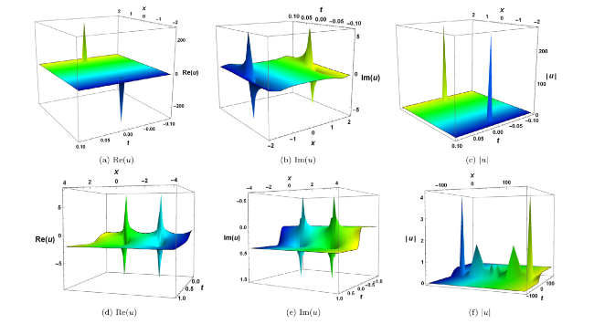
Fig. 2. Interaction of solitons with kink wave for the solution (40) with the choice of parameter (a)-(b)-(c) b0=−4i with the range space −2≤x≤2,−0.1≤t≤0.1, (d) b0=2i+1 with the range space −4≤x≤4,−0.3≤t≤1, (e) b0=7i with the range space −4≤x≤4,−1≤t≤1,(f) b0=2i+5 with the range space −150≤x≤150,−140≤t≤140. |
Figure (3) illustrates the interaction of solitons with kink wave for the real part, imaginary part and absolute value of the solution (41) with the choice of parameter (a) b0=−3i with the range space −4≤x≤4,−1≤t≤1, (b) b0=−8.03−4i with the range space −0.2≤x≤0.2,−1≤t≤1, (c) b0=−4i+4 with the range space −4≤x≤4,−5≤t≤4 respectively.
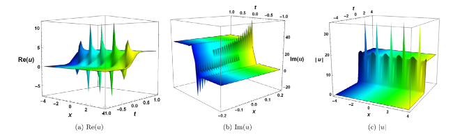
Fig. 3. Interaction of solitons with kink wave for the solution (41) with the choice of parameter (a) b0=−3i with the range space −4≤x≤4,−1≤t≤1, (b) b0=−8.03−4i with the range space −0.2≤x≤0.2,−1≤t≤1, (c) b0=−4i+4 with the range space −4≤x≤4,−5≤t≤4. |
Figure (4) display three different soliton profiles for the real part, imaginary part and absolute value of solution (42) with the choice of parameter (a) b0=−6.2i with the range space −11≤x≤11,−1.5≤t≤1.7, (b) b0=−2i+3 with the range space −13≤x≤3,−1.2≤t≤1, (c) b0=−2i+13 with the range space −12≤x≤12,−1.2≤t≤1 respectively.
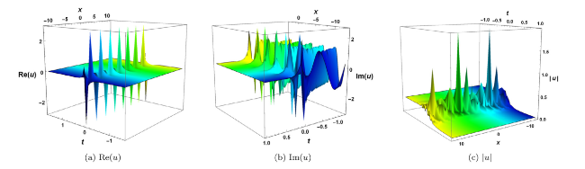
Fig. 4. Different soliton profiles for the solution (42) with the choice of parameter (a) b0=−6.2i with the range space −11≤x≤11,−1.5≤t≤1.7, (b) b0=−2i+3 with the range space −13≤x≤3,−1.2≤t≤1, (c) b0=−2i+13 with the range space −12≤x≤12,−1.2≤t≤1. |
Figure (5) showing the interaction of solitons with kink wave for the real part, imaginary part and absolute value of the solution (74) with the choice of parameter (a) $\epsilon =-1$, ${{\lambda }_{3}}=2$, ${{\lambda }_{4}}=23$, ${{b}_{0}}=0.5$, ${{b}_{1}}=9.7$, $p=-1+7i$, ${{c}_{0}}=2$, ${{c}_{1}}=16$, $G=0.0094$,F=5.7 with the range space −10≤x≤10,−10≤t≤0.10, (b)$\epsilon =-1$, ${{\lambda }_{3}}=2$, ${{\lambda }_{4}}=23$, ${{b}_{0}}=0.5$, ${{b}_{1}}=9.7$, $p=-1+7i$, ${{c}_{0}}=2$, ${{c}_{1}}=16$, G=0.0094, F=5.7 with the range space −10≤x≤10,−10≤t≤0.10, (c) $\epsilon =-1$, ${{\lambda }_{3}}=2$, ${{\lambda }_{4}}=23$, ${{b}_{0}}=0.5$, ${{b}_{1}}=8.7$, $p=-1+7i$, ${{c}_{0}}=2$, ${{c}_{1}}=16$, G=0.0094, F=5.7 with the range space −10≤x≤10,−10≤t≤0.10 respectively.

Fig. 5. Interaction of solitons with kink wave for the solution (74) with the choice of parameter (a) $\epsilon =-1$, ${{\lambda }_{3}}=2$, ${{\lambda }_{4}}=23$, ${{b}_{0}}=0.5$, ${{b}_{1}}=8.7$, $p=-1+7i$, ${{c}_{0}}=2$, ${{c}_{1}}=16$,G=0.0094,F=5.7 with the range space −10≤x≤10,−10≤t≤0.10, (b) $\epsilon =-1$, ${{\lambda }_{3}}=2$, ${{\lambda }_{4}}=23$, ${{b}_{0}}=0.5$, ${{b}_{1}}=9.7$, $p=-1+7i$, ${{c}_{0}}=2$, ${{c}_{1}}=16$,G=0.0094, F=5.7 with the range space −10≤x≤10,−10≤t≤0.10, (c) $\epsilon =-1$, ${{\lambda }_{3}}=2$, ${{\lambda }_{4}}=23$, ${{b}_{0}}=0.5$, ${{b}_{1}}=9.7$, $p=-1+7i$, ${{c}_{0}}=2$, ${{c}_{1}}=16$,G=0.0094,F=5.7 with the range space −10≤x≤10,−10≤t≤0.10. |
Figure (6) demonstrate interaction of solitons with kink wave for real part, imaginary part and absolute value of the solution (79) with the choice of parameter (a) $\epsilon =-1$, ${{b}_{0}}=0.2$, ${{b}_{1}}=0.07$, $p=-1+7i$, ${{c}_{0}}=2$, ${{c}_{1}}=16$ with the range space −12≤x≤12,−2≤t≤2, (b) $\epsilon =-1$, ${{b}_{0}}=0.2$, ${{b}_{1}}=0.07$, $p=-1+7i$, ${{c}_{0}}=2$, ${{c}_{1}}=16$ with the range space −7≤x≤7,−10≤t≤10, (c) $\epsilon =-1$, ${{b}_{0}}=2$, ${{b}_{1}}=7$, $p=-1+i$, ${{c}_{0}}=2$, ${{c}_{1}}=16$ with the range space −7≤x≤7,−10≤t≤10 respectively.
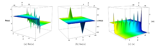
Fig. 6. Interaction of solitons with kink wave for the solution (79) with the choice of parameter (a) $\epsilon =-1$, ${{b}_{0}}=0.2$, ${{b}_{1}}=0.07$, $p=-1+7i$, ${{c}_{0}}=2$, ${{c}_{1}}=16$ with the range space −12≤x≤12,−2≤t≤2, (b) $\epsilon =-1$, ${{b}_{0}}=0.2$, ${{b}_{1}}=0.07$, $p=-1+7i$, ${{c}_{0}}=2$, ${{c}_{1}}=16$ with the range space −7≤x≤7,−10≤t≤10, (c) $\epsilon =-1$, ${{b}_{0}}=2$, ${{b}_{1}}=7$, $p=-1+i$, ${{c}_{0}}=2$, ${{c}_{1}}=16$ with the range space −7≤x≤7,−10≤t≤10. |
Figure (7) describes interaction of solitons with kink wave for real part, imaginary part and absolute value of the solution (94) with the choice of parameter (a) $\epsilon =-1$, ${{b}_{0}}=3$,b1=0.2,p=−2+i,c0=2, ${{c}_{1}}=16$,F=0.5,G=23 with the range space −7≤x≤0,−15≤t≤15, (b) $\epsilon =-1$, ${{b}_{0}}=3$,b1=0.04,p=−2+i,c0=2, x${{c}_{1}}=16$,F=20.05,G=0.03 with the range space −8≤x≤8,−2≤t≤2, (c) $\epsilon =-1$, ${{b}_{0}}=2$, ${{b}_{1}}=7$,p=−2+i,c0=2, ${{c}_{1}}=16$,F=0.5,G=23 with the range space −7≤x≤7,−15≤t≤15 respectively.
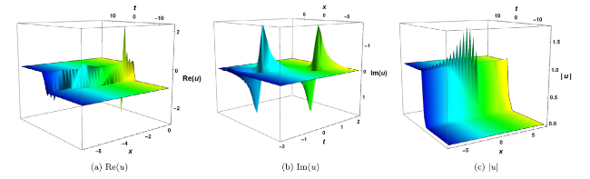
Fig. 7. Interaction of solitons with kink wave for the solution (94) with the choice of parameter (a) $\epsilon =-1$,b0=3,b1=0.2,p=−2+i,c0=2,c1=16,F=0.5,G=23 with the range space −7≤x≤0,−15≤t≤15, (b) $\epsilon =-1$,b0=3,b1=0.04,p=−2+i,c0=2,c1=16,F=20.05,G=0.03 with the range space −8≤x≤8,−2≤t≤2, (c) $\epsilon =-1$,b0=2,b1=7,p=−2+i,c0=2,c1=16,F=0.5,G=23 with the range space −7≤x≤7,−15≤t≤15. |
Figure (8) present solitons profiles for real part, imaginary part and absolute value the solution (95) with the choice of parameter (a) $\epsilon =-1$,b0=5,b1=5,p=−1+3i,c0=2,c1=6,F=0.05,G=0.03 with the range space −1≤x≤1,−2≤t≤2, (b) $\epsilon =-1$,b0=5,b1=5,p=−1+3i,c0=18,c1=6,F=0.05,G=0.03 with the range space −1≤x≤1,−2≤t≤2, (c) $\epsilon =-1$,b0=5,b1=5,p=−1+3i,c0=3.9,c1=6,F=2.05,G=0.03 with the range space −3≤x≤3,−3≤t≤3 respectively.

Fig. 8. Different Soliton profiles for the solution (95) with the choice of parameter (a) $\epsilon =-1$,b0=5,b1=5,p=−1+3i,c0=2,c1=6,F=0.05,G=0.03 with the range space −1≤x≤1,−2≤t≤2, (b) $\epsilon =-1$,b0=5,b1=5,p=−1+3i,c0=18,c1=6,F=0.05,G=0.03 with the range space −1≤x≤1,−2≤t≤2, (c) $\epsilon =-1$,b0=5,b1=5,p=−1+3i,c0=3.9,c1=6,F=2.05,G=0.03 with the range space −3≤x≤.3,−3≤t≤3. |
9. Conclusion
In summary, we successfully applied three efficient techniques, namely the Lie symmetry analysis, the generalized Riccati equation mapping approach, and the modified Kudryashov approach on the nonlinear convection-diffusion-reaction equation, which provide various types of soliton solutions. These resulting soliton solutions involve the exact soliton solutions, inverse function solutions, fractional solutions, traveling wave solutions, dark-soliton solutions, singular-soliton solutions, periodic wave solutions, combo bright-dark soliton solutions, particular solutions, and combo bright-singular soliton solutions. Comparing our results of this paper with the results obtained in [42], [45], [46] by other approaches, we see that all our solutions are new. To the best of the authors's knowledge, these solutions have never been reported before. We exhibit the dynamics of the real part, imaginary part, and absolute part of soliton solutions through 3D graphics which describe their dynamical structures of solitary waves because these solutions belong to the set of complex numbers. The 3D graphics of the solutions demonstrate that all of the methods used are successful, robust, and efficient.
Availability of data and material
Data sharing is not applicable to this article as no data sets were created or analyzed in this study.
Declaration of Competing Interest
The authors declare that they have no conflict of interest.
