
1. Introduction
Many authors have focused their attention in recent years on time dependent variable coefficients nonlinear partial differential equations (NLPDEs) to study the analytic soliton solutions [1], [2], [3], [4], [5], [6], [7], [8], [9], [10], [11], [12], [13], [14], [15], [16], [17], [18], [19], [20], [21], [22], [23], [24], [25], [26], [27]. To comprehend the physical, dynamic, and potential behavior of these NLPDEs, these solutions appear in the form of travelling waves, solitary waves, bright-soliton, dark-soliton, multi-soliton, periodic-soliton, etc. Solitary waves are a sort of natural ocean wave that happens far out at sea and is not induced by land movement. They last only a few seconds, occur in a small region, and are most likely to occur far out at sea. For a long time, many mathematicians and physicists have been studying ocean physics, marine physics, acoustics, plasma physics, nonlinear optics and hydrodynamics [1], [2], [3], [4], [5], [6], [7], [8], [9]. Many methods have been developed in order to establish the solitary wave including travelling wave solutions of the NLPDEs. Some of the analytical methods such as generalized exponential rational function method [1], new $\left( \frac{{{G}'}}{{G}'+G+A} \right)$ -expansion method [2], Lie symmetry method [3], [4], [5], generalized Kudryashov method [6], [7], hetero-Bäcklund transformation via Bell polynomials [8], improved simple equation method and modified F-expansion method [9], $\left( {G}'/G \right)$-expansion method and improved $\left( {G}'/G \right)$-expansion method [10], exp-function method [11], Adomian decomposition method [12], inverse scattering transformation method [13], exponential expansion method [14], $\tan \left( \frac{\phi \left( \xi \right)}{2} \right)$-expansion method [15], modified Jacobi elliptic function expansion method [16], generalized Riccati equation rational expansion method [17], simplified Hirota's method [18], [19], [20], Painlevé analysis [21], [22], [23], [24], auto-Bäcklund transformation [23], [24], [25], [26], [27], are used to solve different models involving NLPDEs.
Recently, Sakovich [28] developed a second order (2+1)-dimensional wave equation
${{u}_{xt}}+{{u}_{yy}}+2u{{u}_{xy}}+6{{u}^{2}}{{u}_{xx}}+2{{\left( {{u}_{xx}} \right)}^{2}}=0.$
Eq. (1.1) is a second degree polynomial in ${{u}_{xx}}$. Sakovich [28] provides the integrability in the form of Painlevé analysis of Eq. (1.1).
Later, Wazwaz [29] extended and proposed (2+1) and (3+1)-dimensional Sakovich equations
${{u}_{xt}}+{{u}_{yy}}+2u{{u}_{xy}}+6{{u}^{2}}{{u}_{xx}}+2{{\left( {{u}_{xx}} \right)}^{2}}+{{u}_{xx}}+{{u}_{xy}}=0,$
And
${{u}_{xt}}+{{u}_{yy}}+2u{{u}_{xy}}+6{{u}^{2}}{{u}_{xx}}+2{{\left( {{u}_{xx}} \right)}^{2}}+{{u}_{xx}}+{{u}_{xy}}+{{u}_{xz}}+{{u}_{yz}}=0,$
respectively by adding two second order term ${{u}_{xx}}$ and ${{u}_{xy}}$ to Eq. (1.1) and introduced a new (3+1)-dimensional Sakovich Eq. (1.3) by adding two more terms ${{u}_{xz}}$ and ${{u}_{yz}}$ to Eq. (1.2).
This paper considers the generalization of Eqs. (1.2) and (1.3) with the time dependent variable coefficients as:
$\begin{align} & {{\wp }_{1}}\left( t \right){{u}_{xt}}+{{\wp }_{2}}\left( t \right){{u}_{yy}}+2{{\wp }_{3}}\left( t \right)u{{u}_{xy}}+6{{\wp }_{4}}\left( t \right){{u}^{2}}{{u}_{xx}}+2{{\wp }_{5}}\left( t \right){{\left( {{u}_{xx}} \right)}^{2}} \\ & +{{\wp }_{6}}\left( t \right){{u}_{xx}}+{{\wp }_{7}}\left( t \right){{u}_{xy}}=0, \\ \end{align}$
$\begin{align} & {{\wp }_{1}}\left( t \right){{u}_{xt}}+{{\wp }_{2}}\left( t \right){{u}_{yy}}+2{{\wp }_{3}}\left( t \right)u{{u}_{xy}}+6{{\wp }_{4}}\left( t \right){{u}^{2}}{{u}_{xx}}+2{{\wp }_{5}}\left( t \right){{\left( {{u}_{xx}} \right)}^{2}} \\ & +{{\wp }_{6}}\left( t \right){{u}_{xx}}+{{\wp }_{7}}\left( t \right){{u}_{xy}}+{{\wp }_{8}}\left( t \right){{u}_{xz}}+{{\wp }_{9}}\left( t \right){{u}_{yz}}=0, \\ \end{align}$
Where ${{\wp }_{1}}\left( t \right)$, ${{\wp }_{2}}\left( t \right)$, ${{\wp }_{3}}\left( t \right)$, ${{\wp }_{4}}\left( t \right)$, ${{\wp }_{5}}\left( t \right)$, ${{\wp }_{6}}\left( t \right)$, ${{\wp }_{7}}\left( t \right)$, ${{\wp }_{8}}\left( t \right)$ and ${{\wp }_{9}}\left( t \right)$ are arbitrary analytic functions of t, and $u\left( x,y,t \right)$ be the wave amplitude in the Eq. (1.4) however $u\left( x,y,z,t \right)$ is the wave amplitude in the Eq. (1.5). The time dependent variable coefficients (2+1) and (3+1)-dimensional extended Sakovich Eqs. (1.4) and (1.5) share various features in common and are the key feature in the field of ocean physics as both equations possess the solitary wave soliton solutions. The time-dependent variable coefficients generalization of Eqs. (1.4) and (1.5) has not been done before, hence this depicts the novelty of this paper.
This article motivates to find the integrability features such as leading order analysis, resonance values and arbitrary functions to verify the compatibility conditions of two considered Eqs. (1.4) and (1.5). Another motivation is to explore various analytic solutions of these two equations. The purpose of this paper is to divulge these motives.
The Painlevé analysis method [21], [22], [23], [24] is being adopted to test the integrability of the considered equations while an auto-Bäcklund transformation (ABT) method [23], [24], [25], [26], [27] is being discussed to obtain the analytic solutions for Eqs. (1.4) and (1.5) in this article. The most often used method for generating the ABT is the truncated Painlevé expansion approach. Both the methods are completely algorithmic and computational. It has been noticed that the ABT method is more powerful, effective and easy to implementable for finding different kind of analytic solutions including kink-soliton, kink-antikink soliton, periodic-soliton, bright-soliton, dark-soliton etc. A variety of nonlinear evolution equations like as modified KdV equation with variable coefficients [23], (3+1)-dimensional Hirota-Satsuma-Ito-like system [24], generalized variable-coefficient Korteweg-de Vries (KdV) equation [25], (3+1)-dimensional generalised Yu-Toda-Sasa-Fukuyama equation [26], (3+1)-dimensional Boiti-Leon-Manna-Pempinelli equation [27] etc. are studied by using the ABT method. In addition, it has been shown different dynamics of solitary wave solutions in the form of 3D and 2D graphics. Moreover, the developmental dynamics of the resulting solitary wave solutions are noteworthy, and that they might be useful in the study of complex physical problems.
This manuscript is systematized as follows: In Section 2, Painlevé analysis is briefly discussed. The integrability components such as leading order behaviour, resonances and compatibility criteria for Eqs. (1.4) and (1.5) are investigated in Sections 3 and 4 respectively. Whereas Sections 5 and 6 give the mathematical methodology to derive the exact solutions of (2+1) and (3+1)-dimensional variable coefficients extended Sakovich equations by the ABT method respectively. Section 7 explains the physical application of the graphs, and Section 8 draws a precise and clear conclusion.
2. Brief description of Painlevé analysis
The truncated Painlevé expansion approach is used to investigate the precise soliton solution for the NLPDEs, while the Painlevé analysis [21], [22], [23], [24] is used to evaluate whether a NLPDE is integrable. The Painlevé test is satisfied when a PDE's single-valued solutions contain no bad singularities other than moveable poles about a singular manifold g.
Considering a NLPDE
$S\left( u,{{u}_{{{w}_{1}}}},{{u}_{{{w}_{2}}}},{{u}_{{{w}_{1}}{{w}_{2}}}},{{u}_{{{w}_{1}}{{w}_{1}}}},{{u}_{{{w}_{2}}{{w}_{2}}}},\cdots \right)=0.$
The singular manifold is defined by
$g\left( {{w}_{1}},{{w}_{2}},\ldots,{{w}_{n}} \right)=0.$
The solution for Eq. (2.1) is considered by Laurent series as
$u\left( {{w}_{1}},{{w}_{2}},\ldots,{{w}_{n}} \right)={{g}^{\alpha }}\left( {{w}_{1}},{{w}_{2}},\ldots,{{w}_{n}} \right)\underset{j=0}{\overset{\infty }{\mathop \sum }}\,{{u}_{j}}\left( {{w}_{1}},{{w}_{2}},\ldots,{{w}_{n}} \right){{g}^{j}}\times \left( {{w}_{1}},{{w}_{2}},\ldots,{{w}_{n}} \right),$
where $u$ and ${{u}_{j}}$'s are the arbitrary functions of $\left( {{w}_{1}},{{w}_{2}},\ldots,{{w}_{n}} \right)$ and $\alpha $ is negative. The steps in this method are as follows::
• The value of $\alpha $ can be determined by plugging
$u={{g}^{\alpha }}{{u}_{0}},$
into Eq. (2.1).
• Solving the occurring equation for non-zero ${{u}_{0}}$ by equating the coefficient of leading term to zero. This may conduct the various branch.
•Substituting
$u={{u}_{0}}{{g}^{\alpha }}+\underset{j=1}{\overset{\infty }{\mathop \sum }}\,{{u}_{j}}{{g}^{j+\alpha }},$
into Eq. (2.1). This gives the values of j which are called resonances.
• The series given by Eq. (2.3) will always be expanded at the highest resonance value $j={{r}_{\max }}$,
$u={{g}^{\alpha }}\underset{j=0}{\overset{{{r}_{\max }}}{\mathop \sum }}\,{{u}_{j}}{{g}^{j}}.$
Next to calculate the values of 's functions.
• The compatibility criteria for the Painlevé test is that the coefficients ${{u}_{j}}$ corresponds to resonance values would occur as arbitrary function. If the compatibility criteria is fulfilled at the resonance values, then Eq. (2.1) passes the Painlevé test and Eq. (2.1) is Painlevé integrable.
3. Painlevé analysis of (2+1)-dimensional extended Sakovich equation with time dependent variable coefficients
In the present analysis, Weiss, Tabor and Carnevale (WTC) developed an algorithm in Weiss et al. [30] to test the Painlevé integrability for the NLPDEs. The solution of a NLPDE is represented as a meromorphic function with regard to x, y, and t in the WTC method, and the singular manifold is presented by
$g\left( x,y,t \right)=0.$
The solution of Eq. (1.4) is defined by the Laurent series,
$u={{g}^{\alpha }}\underset{j=0}{\overset{\infty }{\mathop \sum }}\,{{u}_{j}}{{g}^{j}},$
where $u$, ${{u}_{j}}$'s and g are the functions of x, y, and t and $\alpha $ is a negative integer provided that ${{u}_{0}}\ne 0$.
The values of $\alpha $ and ${{u}_{0}}$ are determined by substituting $u={{u}_{0}}{{g}^{\alpha }}$ into Eq. (1.4). One gets
$\alpha =-2,\qquad {{u}_{0}}=\frac{-2{{\wp }_{5}}\left( t \right)g_{x}^{2}}{{{\wp }_{4}}\left( t \right)}.$
Here the recursion relation is obtained by substituting full Laurent series
$u={{u}_{0}}{{g}^{-2}}+\underset{j=1}{\overset{\infty }{\mathop \sum }}\,{{u}_{j}}{{g}^{j-2}},$
into Eq. (1.4).
Resonance values are calculated by equating the coefficient of ${{g}^{j-8}}$ to zero. This gives ${{j}^{2}}-5j-6=0$.
Therefore the resonance values are j=-1,6.
The highest resonance value is j=6 which leads to truncate the Laurent series given in Eq. (3.4) as
$u={{u}_{0}}{{g}^{-2}}+{{u}_{1}}{{g}^{-1}}+{{u}_{2}}+{{u}_{3}}g+{{u}_{4}}{{g}^{2}}+{{u}_{5}}{{g}^{3}}+{{u}_{6}}{{g}^{4}}.$
Now plugging Eq. (3.5) into Eq. (1.4) and equate like exponents of g to zero, give the following coefficients
${{u}_{1}}=\frac{2{{\wp }_{5}}\left( t \right){{g}_{xx}}}{{{\wp }_{4}}\left( t \right)},$
${{u}_{2}}=\frac{-{{\wp }_{3}}\left( t \right){{g}_{y}}{{g}_{x}}+3{{\wp }_{5}}\left( t \right)g_{xx}^{2}-4{{\wp }_{5}}\left( t \right){{g}_{x}}{{g}_{xxx}}}{6{{\wp }_{4}}\left( t \right)g_{x}^{2}},$
$\begin{align} & {{u}_{3}}=\frac{1}{6{{\wp }_{4}}\left( t \right)g_{x}^{4}}({{\wp }_{3}}\left( t \right)g_{x}^{2}{{g}_{xy}}-{{\wp }_{3}}\left( t \right){{g}_{y}}{{g}_{x}}{{g}_{xx}}+3{{\wp }_{5}}\left( t \right)g_{xx}^{3} \\ & -4{{\wp }_{5}}\left( t \right){{g}_{x}}{{g}_{xx}}{{g}_{xxx}}+{{\wp }_{5}}\left( t \right)g_{x}^{2}{{g}_{xxxx}}), \\ \end{align}$
$\begin{align} & {{u}_{4}}=\frac{1}{120{{\wp }_{4}}(t){{\wp }_{5}}(t)g_{x}^{6}}\left( -{{\wp }_{3}}{{(t)}^{2}}g_{y}^{2}g_{x}^{2}+6{{\wp }_{2}}(t){{\wp }_{4}}(t)g_{y}^{2}g_{x}^{2} \right. \\ & +6{{\wp }_{1}}(t){{\wp }_{4}}(t){{g}_{t}}g_{x}^{3}+6{{\wp }_{4}}(t){{\wp }_{7}}(t){{g}_{y}}g_{x}^{3}+6{{\wp }_{4}}(t){{\wp }_{6}}(t)g_{x}^{4} \\ & +30{{\wp }_{3}}(t){{\wp }_{5}}(t)g_{x}^{2}{{g}_{xy}}{{g}_{xx}}-30{{\wp }_{3}}(t){{\wp }_{5}}(t){{g}_{y}}{{g}_{x}}g_{xx}^{2}+75{{\wp }_{5}}{{(t)}^{2}}g_{xx}^{4} \\ & -10{{\wp }_{3}}(t){{\wp }_{5}}(t)g_{x}^{3}{{g}_{xxy}}+10{{\wp }_{3}}(t){{\wp }_{5}}(t){{g}_{y}}g_{xxx}^{2}-120{{\wp }_{5}}{{(t)}^{2}}{{g}_{x}}g_{xx}^{2}{{g}_{xxx}} \\ & +20{{\wp }_{5}}{{(t)}^{2}}g_{x}^{2}g_{xxx}^{2}+30{{\wp }_{5}}{{(t)}^{2}}g_{x}^{2}{{g}_{xx}}{{g}_{xxx}}\left. -4{{\wp }_{5}}{{(t)}^{2}}g_{x}^{3}{{g}_{xxxxx}} \right) \\ \end{align}$
$\begin{aligned} u_{5}= & \frac{1}{360 \wp_{4}(t) \wp_{5}(t)^{2} g_{x}^{8}}\left(-10 \wp_{2}(t) \wp_{4}(t) \wp_{5}(t) g_{y y} g_{x}^{4}\right. \\ & +10 \wp_{1}(t) \wp_{5}(t) \wp_{4}^{\prime}(t) g_{x}^{5}-10 \wp_{1}(t) \wp_{4}(t) \wp_{5}^{\prime}(t) g_{x}^{5} \\ & -18 \wp_{1}(t) \wp_{4}(t) \wp_{5}(t) g_{x}^{4} g_{x t}+6 \wp_{3}(t)^{2} \wp_{5}(t) g_{y} g_{x}^{3} g_{x y} \\ & -16 \wp_{2}(t) \wp_{4}(t) \wp_{5}(t) g_{y} g_{x}^{3} g_{x y}-1 \wp_{4}(t) \wp_{5}(t) \wp_{7}(t) g_{x}^{4} g_{x y} \\ & -9 \wp_{3}(t)^{2} \wp_{5}(t) g_{y}^{2} g_{x}^{2} g_{x x}+44 \wp_{2}(t) \wp_{4}(t) \wp_{5}(t) g_{y}^{2} g_{x}^{2} g_{x x} \\ & +36 \wp_{1}(t) \wp_{4}(t) \wp_{5}(t) g_{t} g_{x}^{3} g_{x x}+36 \wp_{4}(t) \wp_{5}(t) \wp_{7}(t) g_{y} g_{x}^{3} g_{x x} \\ & +18 \wp_{4}(t) \wp_{5}(t) \wp_{6}(t) g_{x}^{4} g_{x x}+150 \wp_{3}(t) \wp_{5}(t)^{2} g_{x}^{2} g_{x y} g_{x x}^{2} \\ & -150 \wp_{3}(t) \wp_{5}(t)^{2} g_{y} g_{x} g_{x x}^{3}+31 \wp_{5}(t)^{3} g_{x x}^{5}-60 \wp_{3}(t) \wp_{5}(t)^{2} g_{x}^{3} g_{x x} g_{x x y} \\ & -40 \wp_{3}(t) \wp_{5}(t)^{2} g_{x}^{3} g_{x y} g_{x x x}+100 \wp_{3}(t) \wp_{5}(t)^{2} g_{y} g_{x}^{2} g_{x x} g_{x x x} \\ & -600 \wp_{5}(t)^{3} g_{x} g_{x x}^{3} g_{x x x}+200 \wp_{5}(t)^{3} g_{x}^{2} g_{x x} g_{x x x}^{2}+10 \wp_{3}(t) \wp_{5}(t)^{2} \\ & g_{x}^{4} g_{x x x y}-10 \wp_{3}(t) \wp_{5}(t)^{2} g_{y} g_{x}^{3} g_{x x x x}+150 \wp_{5}(t)^{3} g_{x}^{2} g_{x x}^{2} g_{x x x x} \\ & \left.-40 \wp_{5}(t)^{3} g_{x}^{3} g_{x x x} g_{x x x x}-24 \wp_{5}(t)^{3} g_{x}^{3} g_{x x} g_{x x x x x}+2 \wp_{5}(t)^{3} g_{x}^{4} g_{x x x x x x}\right).\end{aligned}$
As usual, the resonance at negative value i.e. j=-1 occurs as arbitrary about the singular manifold $g(x,y,t)=0$. The coefficient of ${{g}^{-2}}$ corresponds to the resonance value at j=6 is obtained as zero which demonstrates that ${{u}_{6}}$ is an arbitrary function. Therefore the compatibility criteria of Painlevé test is satisfied. Thus Eq. (1.4) is Painlevé integrable.
4. Painlevé analysis of (3+1)-dimensional extended Sakovich equation with time dependent variable coefficients
Proceed as in previous section to find the Painlevé property of Eq. (1.5) about the singular manifold given by Eq. (2.2). Consider the solution of Eq. (1.5) by the Laurent series expansion given in Eq. (2.3) about the singular manifold g, where $u=u(x,y,z,t)$ is the solution of Eq. (1.5).
The values $\alpha $ and ${{u}_{0}}$ of leading orders can be determined by substituting $u={{u}_{0}}{{g}^{\alpha }}$ into Eq. (1.5). This gives
$\alpha =-2,\qquad {{u}_{0}}=\frac{-2{{\wp }_{5}}\left( t \right)g_{x}^{2}}{{{\wp }_{4}}\left( t \right)}.$
Here the recursion relation is obtained by substituting
$u={{u}_{0}}{{g}^{-2}}+\underset{j=1}{\overset{\infty }{\mathop \sum }}\,{{u}_{j}}{{g}^{j-2}},$
into Eq. (1.5).
Resonance values are evaluated by equating the coefficient of ${{g}^{j-8}}$ to zero, which gives the quadratic polynomial in j as
J2-5j-6=0
Therefore the resonance values are at j=-1,6, the highest resonance value is j=6 which leads to truncate the Laurent series given in Eq. (4.2) as
$u={{u}_{0}}{{g}^{-2}}+{{u}_{1}}{{g}^{-1}}+{{u}_{2}}+{{u}_{3}}g+{{u}_{4}}{{g}^{2}}+{{u}_{5}}{{g}^{3}}+{{u}_{6}}{{g}^{4}}.$
On substituting Eq. (4.3) into Eq. (1.5) and equate like exponents of g to zero, give the following coefficients,
${{u}_{1}}=\frac{2{{\wp }_{5}}\left( t \right){{g}_{xx}}}{{{\wp }_{4}}\left( t \right)},$
${{u}_{2}}=\frac{-{{\wp }_{3}}\left( t \right){{g}_{y}}{{g}_{x}}+3{{\wp }_{5}}\left( t \right)g_{xx}^{2}-4{{\wp }_{5}}\left( t \right){{g}_{x}}{{g}_{xxx}}}{6{{\wp }_{4}}\left( t \right)g_{x}^{2}},$
$\begin{align} & {{u}_{3}}=\frac{1}{6\;{{\wp }_{4}}\left( t \right)g_{x}^{4}}({{\wp }_{3}}\left( t \right)g_{x}^{2}{{g}_{xy}}-{{\wp }_{3}}\left( t \right){{g}_{y}}{{g}_{x}}{{g}_{xx}}+3{{\wp }_{5}}\left( t \right)g_{xx}^{3} \\ & -4\;{{\wp }_{5}}\left( t \right){{g}_{x}}{{g}_{xx}}{{g}_{xxx}}+{{\wp }_{5}}\left( t \right)g_{x}^{2}{{g}_{xxxx}}), \\ \end{align}$
$\begin{aligned} u_{4}= & \frac{1}{120 \wp_{4}(t) \wp_{5}(t) g_{x}^{6}}\left(6 \wp_{4}(t) \wp_{9}(t) g_{z} g_{y} g_{x}^{2}-\wp_{3}(t)^{2} g_{y}^{2} g_{x}^{2}\right. \\ & +6 \wp_{2}(t) \wp_{4}(t) g_{y}^{2} g_{x}^{2}+6 \wp_{1}(t) \wp_{4}(t) g_{t} g_{x}^{3}+6 \wp_{4}(t) \wp_{8}(t) g_{z} g_{x}^{3} \\ & +6 \wp_{4}(t) \wp_{7}(t) g_{y} g_{x}^{3}+6 \wp_{4}(t) \wp_{6}(t) g_{x}^{4}+3 \wp_{3}(t) \wp_{5}(t) g_{x}^{2} g_{x y} g_{x x} \\ & -30 \wp_{3}(t) \wp_{5}(t) g_{y} g_{x} g_{x x}^{2}+75 \wp_{5}(t)^{2} g_{x x}^{4}-10 \wp_{3}(t) \wp_{5}(t) g_{x}^{3} g_{x x y} \\ & +10 \wp_{3}(t) \wp_{5}(t) g_{y} g_{x}^{2} g_{x x x}-12 \wp_{5}(t)^{2} g_{x} g_{x x}^{2} g_{x x x}+2 \wp_{5}(t)^{2} g_{x}^{2} g_{x x x}^{2} \\ & \left.+30 \wp_{5}(t)^{2} g_{x}^{2} g_{x x} g_{x x x x}-4 \wp_{5}(t)^{2} g_{x}^{3} g_{x x x x x}\right), \end{aligned}$
$\begin{aligned} u_{5}= & \frac{1}{360 \wp_{4}(t) \wp_{5}(t)^{2} g_{x}^{8}}\left(-10 \wp_{4}(t) \wp_{9}(t) \wp_{5}(t) g_{y z} g_{x}^{4}-10 \wp_{2}(t) \wp_{4}(t) \wp_{5}(t) g_{y y} g_{x}^{4}\right. \\ & +10 \wp_{1}(t) \wp_{5}(t) \wp_{4}^{\prime}(t) g_{x}^{5} \\ & -10 \wp_{1}(t) \wp_{4}(t) \wp_{5}^{\prime}(t) g_{x}^{5}-18 \wp_{1}(t) \wp_{4}(t) \wp_{5}(t) g_{x}^{4} g_{x t} \\ & -8 \wp_{4}(t) \wp_{9}(t) \wp_{5}(t) g_{y} g_{x}^{3} g_{x z} \\ & -18 \wp_{4}(t) \wp_{5}(t) \wp_{8}(t) g_{x}^{4} g_{x z} \\ & -8 \wp_{4}(t) \wp_{9}(t) \wp_{5}(t) g_{z} g_{x}^{3} g_{x y}+6 \wp_{3}(t)^{2} \wp_{5}(t) g_{y} g_{x}^{3} g_{x y} \\ & -16 \wp_{2}(t) \wp_{4}(t) \wp_{5}(t) g_{y} g_{x}^{3} g_{x y}-1 \wp_{4}(t) \wp_{5}(t) \wp_{7}(t) g_{x}^{4} g_{x y} \\ & +44 \wp_{4}(t) \wp_{9}(t) \wp_{5}(t) g_{z} g_{y} g_{x}^{2} g_{x x}-9 \wp_{3}(t)^{2} \wp_{5}(t) g_{y}^{2} g_{x}^{2} g_{x x} \\ & +44 \wp_{2}(t) \wp_{4}(t) \wp_{5}(t) g_{y}^{2} g_{x}^{2} g_{x x}+36 \\ & +36 \wp_{4}(t) \wp_{5}(t) \wp_{8}(t) g_{z} g_{x}^{3} g_{x x} \wp_{1}(t) \wp_{4}(t) \wp_{5}(t) g_{t} g_{x}^{3} g_{x x} \\ & +36 \wp_{4}(t) \wp_{5}(t) \wp_{7}(t) g_{y} g_{x}^{3} g_{x x}+18 \wp_{4}(t) \wp_{5}(t) \wp_{6}(t) g_{x}^{4} g_{x x} \\ & +150 \wp_{3}(t) \wp_{5}(t)^{2} g_{x}^{2} g_{x y} g_{x x}^{2}-150 \wp_{3}(t) \wp_{5}(t)^{2} g_{y} g_{x} g_{x x}^{3} \\ & +31 \wp_{5}(t)^{3} g_{x x}^{5}-60 \wp_{3}(t) \wp_{5}(t)^{2} g_{x}^{3} g_{x x} g_{x x y} \\ & -40 \wp_{3}(t) \wp_{5}(t)^{2} g_{x}^{3} g_{x y} g_{x x x}+100 \wp_{3}(t) \wp_{5}(t)^{2} g_{y} g_{x}^{2} g_{x x} g_{x x x} \\ & -600 \wp_{5}(t)^{3} g_{x} g_{x x}^{3} g_{x x x}+200 \wp_{5}(t)^{3} g_{x}^{2} g_{x x} g_{x x x}^{2} \\ & +10 \wp_{3}(t) \wp_{5}(t)^{2} g_{x}^{4} g_{x x x y}-10 \wp_{3}(t) \wp_{5}(t)^{2} g_{y} g_{x}^{3} g_{x x x x} \\ & +150 \wp_{5}(t)^{3} g_{x}^{2} g_{x x}^{2} g_{x x x x}-40 \wp_{5}(t)^{3} g_{x}^{3} g_{x x x} g_{x x x x} \\ & \left.-24 \wp_{5}(t)^{3} g_{x}^{3} g_{x x} g_{x x x x x}+2 \wp_{5}(t)^{3} g_{x}^{4} g_{x x x x x}\right). \end{aligned}$
As usual, the resonance at negative value i.e. j=-1 occurs as arbitrary about the singular manifold $g(x,y,z,t)=0$. The coefficient of ${{g}^{-2}}$ corresponds to the resonance value at j=6 is obtained as zero which demonstrates that ${{u}_{6}}$ is an arbitrary function. Therefore the compatibility criteria of Painlevé test is satisfied. Thus Eq. (1.5) is Painlevé integrable.
5. Auto-Bäcklund transformation and exact solutions of (2+1)-dimensional Sakovich equation with time dependent variable coefficients
$u={{u}_{0}}{{g}^{-2}}+{{u}_{1}}{{g}^{-1}}+{{u}_{2}}.$
On plugging Eq. (5.1) into Eq. (1.4) yields
$\begin{aligned} g^{-8}: & 36 \wp_{4}(t) u_{0}^{3} g_{x}^{2}+72 \wp_{5}(t) u_{0}^{2} g_{x}^{4}=0. \\ & \text { Thus, } \quad u_{0}=\frac{-2 \wp_{5}(t) g_{x}^{2}}{\wp_{4}(t)}, \end{aligned}$
$\begin{array}{c} g^{-7}: \quad \frac{24 \wp_{\wp_{5}}(t)^{2} u_{1} g_{x}^{6}}{\wp_{4}(t)}-\frac{480 \wp_{5}(t)^{3} g_{x}^{6} g_{x x}}{\wp_{4}(t)^{2}}=0. \\ \text { Thus, } \quad u_{1}=\frac{2 \wp_{5}(t) g_{x x}}{\wp_{4}(t)}, \end{array}$
${{g}^{-6}}:\ \frac{1}{{{\wp }_{4}}{{\left( t \right)}^{2}}}48{{\wp }_{5}}{{\left( t \right)}^{2}}g_{x}^{4}\left( {{\wp }_{3}}\left( t \right){{g}_{y}}{{g}_{x}}+6{{\wp }_{4}}\left( t \right){{u}_{2}}g_{x}^{2}+{{\wp }_{5}}\left( t \right)\left( -3g_{xx}^{2}+4{{g}_{x}}{{g}_{xxx}} \right) \right)=0,$
$\begin{align} & {{g}^{-5}}:\frac{1}{{{\wp }_{4}}{{\left( t \right)}^{2}}}48{{\wp }_{5}}{{\left( t \right)}^{2}}g_{x}^{2}(18{{\wp }_{4}}\left( t \right){{u}_{2}}g_{x}^{2}{{g}_{xx}}+{{\wp }_{3}}\left( t \right){{g}_{x}}({{g}_{x}}{{g}_{xy}} \\ & +2{{g}_{y}}{{g}_{xx}})+{{\wp }_{5}}\left( t \right)(-6g_{xx}^{3}+8{{g}_{x}}{{g}_{xx}}{{g}_{xxx}}+g_{x}^{2}{{g}_{xxxx}}))=0, \\ \end{align}$
$\begin{aligned} g^{-4}: & \frac{1}{\wp_{4}(t)^{2}} 4 \wp_{5}(t)\left(-3 \wp_{2}(t) \wp_{4}(t) g_{y}^{2} g_{x}^{2}-3 \wp_{1}(t) \wp_{4}(t) g_{t} g_{x}^{3}\right. \\ & -3 \wp_{4}(t) \wp_{7}(t) g_{y} g_{x}^{3}-6 \wp_{3}(t) \wp_{4}(t) u_{2} g_{y} g_{x}^{3}-3 \\ & \wp_{4}(t) \wp_{6}(t) g_{x}^{4}-18 \wp_{4}(t)^{2} u_{2}^{2} g_{x}^{4}+18 \wp_{3}(t) \wp_{5}(t) g_{x}^{2} g_{x y} g_{x x} \\ & +12 \wp_{3}(t) \wp_{5}(t) g_{y} g_{x} g_{x x}^{2}+180 \wp_{4}(t) \wp_{5}(t) u_{2} \\ & g_{x}^{2} g_{x x}^{2}-18_{\wp_{5}}(t)^{2} g_{x x}^{4}-6_{4}(t) \wp_{5}(t) g_{x}^{4} u_{2, x x} \\ & +6 \wp_{3}(t) \wp_{5}(t) g_{x}^{3} g_{x x y}+2 \wp_{3}(t) \wp_{5}(t) g_{y} g_{x}^{2} g_{x x x}+48 \wp_{4}(t) \\ & \left.\wp_{5}(t) u_{2} g_{x}^{3} g_{x x x}+32 \wp_{5}(t)^{2} g_{x}^{2} g_{x x x}^{2}+24 \wp_{5}(t)^{2} g_{x}^{2} g_{x x} g_{x x x x}\right)=0, \end{aligned}$
$\begin{aligned} g^{-3}: & \frac{4}{\wp_{4}(t)^{2}}\left(\wp _ { 2 } ( t ) \wp _ { 4 } ( t ) \wp _ { 5 } ( t ) \left(g_{y y} g_{x}^{2}+g_{y}\left(4 g_{x} g_{x y}\right.\right.\right. \\ & \left.\left.+g_{y} g_{x x}\right)\right)+\wp_{1}(t) g_{x}\left(\wp_{4}(t) \wp_{5}^{\prime}(t) g_{x}^{2}+\wp_{5}(t)\left(-\wp_{4}^{\prime}(t) g_{x}^{2}\right.\right. \\ & \left.\left.+3 \wp_{4}(t)\left(g_{x} g_{x t}+g_{t} g_{x x}\right)\right)\right)+\wp_{5}(t)\left(36 \wp_{4}(t)^{2} u_{2}^{2} g_{x}^{2} g_{x x}\right. \\ & -2 \wp_{5}(t)\left(\wp _ { 3 } ( t ) \left(3 g_{x y} g_{x x}^{2}+3 g_{x} g_{x x} g_{x x y}+g_{y}\right.\right. \\ & \left.\left.g_{x x} g_{x x x}+g_{x}^{2} g_{x x x y}\right)+8 \wp_{5}(t) g_{x} g_{x x x} g_{x x x x}\right)+3 \wp_{4}(t)\left(\wp _ { 7 } ( t ) g _ { x } \left(g_{x} g_{x y}\right.\right. \\ & \left.+g_{y} g_{x x}\right)+2\left(\wp_{6}(t) g_{x}^{2} g_{x x}+\wp_{3}(t)\right. \\ & u_{2} g_{x}\left(g_{x} g_{x y}+g_{y} g_{x x}\right)-2 \wp_{5}(t)\left(-g_{x}^{2} g_{x x} u_{2, x x}+u_{2}\left(3 g_{x x}^{3}\right.\right. \\ & \left.\left.\left.\left.\left.\left.+4 g_{x} g_{x x} g_{x x x}+g_{x}^{2} g_{x x x x}\right)\right)\right)\right)\right)\right)=0, \end{aligned}$
$\begin{aligned} g^{-2}: & \frac{-2}{\wp_{4}(t)^{2}}\left(-3 \wp_{1}(t) \wp_{5}(t) \wp_{4}^{\prime}(t) g_{x} g_{x x}\right. \\ & +3 \wp_{1}(t) \wp_{4}(t) \wp_{5}^{\prime}(t) g_{x} g_{x x}+3 \wp_{1}(t) \wp_{4}(t) \wp_{5}(t) g_{x t} g_{x x}+3 \wp_{4}(t) \wp_{5}(t) \\ & \wp_{7}(t) g_{x y} g_{x x}+3 \wp_{4}(t) \wp_{5}(t) \wp_{6}(t) g_{x x}^{2}+18_{4}(t)^{2} \wp_{5}(t) u_{2}^{2} g_{x x}^{2} \\ & +12 \wp_{4}(t)^{2} \wp_{5}(t) u_{2} g_{x}^{2} u_{2, x x}+3 \wp_{1}(t) \wp_{4}(t) \\ & \wp_{5}(t) g_{x} g_{x x t}+3 \wp_{4}(t) \wp_{5}(t) \wp_{7}(t) g_{x} g_{x x y}+\wp_{2}(t) \wp_{4}(t) \wp_{5}(t)\left(2 g_{x y}^{2}\right. \\ & \left.+2 g_{x} g_{x y y}+g_{y y} g_{x x}+2 g_{y} g_{x x y}\right)+ \\ & \wp_{1}(t) \wp_{4}(t) \wp_{5}(t) g_{t} g_{x x x}+\wp_{4}(t) \wp_{5}(t) \wp_{7}(t) g_{y} g_{x x x} \\ & +4 \wp_{4}(t) \wp_{5}(t) \wp_{6}(t) g_{x} g_{x x x}+24 \wp_{4}(t)^{2} \wp_{5}(t) u_{2}^{2} g_{x} \\ & g_{x x x}+16 \wp_{4}(t) \wp_{5}(t)^{2} g_{x} u_{2, x x} g_{x x x}+2 \wp_{3}(t) \wp_{5}(t)\left(\wp _ { 4 } ( t ) \left(g_{x}^{2} u_{2, x y}\right.\right. \\ & \left.\left.+3 u_{2} g_{x} g_{x x y}+u_{2}\left(3 g_{x y} g_{x x}+g_{y} g_{x x x}\right)\right)-2 \wp_{5}(t) g_{x x} g_{x x x y}\right) \\ & \left.-24 \wp_{4}(t) \wp_{5}(t)^{2} u_{2} g_{x x} g_{x x x x}-4 \wp_{5}(t)^{3} g_{x x x x}^{2}\right)=0, \end{aligned}$
$\begin{aligned} g^{-1}: & \frac{2}{\wp_{4}(t)^{2}}\left(-\wp_{1}(t) \wp_{5}(t) \wp_{4}^{\prime}(t) g_{x x x}\right. \\ & +2 \wp_{3}(t) \wp_{4}(t) \wp_{5}(t)\left(u_{2, x y} g_{x x}+u_{2} g_{x x x y}\right)+6 \wp_{4}(t)^{2} \wp_{5}(t) u_{2}\left(2 g_{x x}\right. \\ & \left.u_{2, x x}+u_{2} g_{x x x x}\right)+\wp_{4}(t)\left(\wp_{2}(t) \wp_{5}(t) g_{x x y y}+\wp_{1}(t)\left(\wp_{5}^{\prime}(t) g_{x x x}\right.\right. \\ & \left.+\wp_{5}(t) g_{x x x t}\right)+\wp_{5}(t)\left(\wp_{7}(t) g_{x x x y}\right. \\ & \left.\left.\left.+\left(\wp_{6}(t)+4 \wp_{5}(t) u_{2, x x}\right) g_{x x x x}\right)\right)\right)=0, \end{aligned}$
$\begin{aligned} g^{0}: & \wp_{2}(t) u_{2, y y}+\wp_{1}(t) u_{2, x t}+\wp_{7}(t) u_{2, x y}+2 \wp_{3}(t) u_{2} u_{2, x y} \\ & +\wp_{6}(t) u_{2, x x}+6 \wp_{4}(t) u_{2}^{2} u_{2, x x}+2 \wp_{5}(t) u_{2, x x}^{2} \\ & =0. \end{aligned}$
Clearly, g satisfies Eqs. (5.4)–(5.10) and ${{u}_{2}}$ is a solution of Eq. (1.4), provided that ${{\wp }_{4}}(t)\ne 0$ and ${{g}_{x}}\ne 0$.
Hence, an ABT for Eq. (1.4) is generated as
$u=\frac{2{{\wp }_{5}}\left( t \right)}{{{\wp }_{4}}\left( t \right)}\frac{{{\partial }^{2}}}{\partial {{x}^{2}}}\left( \ln g \right)+{{u}_{2}}.$
Eq. (5.11) produces various analytic solution solution for the particular values of and.
Here two families of analytic solutions for Eq. (1.4) are derived by opting the particular forms of g and ${{u}_{2}}$ via following two cases:
Case 1:
Consider
$g\left( x,y,t \right)=\ 1+{{e}^{p\left( t \right)x+r\left( t \right)}},$
${{u}_{2}}\left( x,y,t \right)=\ f\left( t \right)x+w\left( t \right),$
where $p(\ne 0)$, r, f and $w$ are arbitrary functions of t. The system of equations is obtained by substituting Eqs. (5.12) and (5.13) into the Eqs. (5.4)–(5.10) as
${{\wp }_{5}}\left( t \right)p{{\left( t \right)}^{2}}+6{{\wp }_{4}}\left( t \right)\left( xf\left( t \right)+w\left( t \right) \right)=0,$
$\begin{array}{l} 38 \wp_{5}(t)^{2} p(t)^{5}-18 \wp_{4}(t)^{2} p(t)(x f(t)+w(t))^{2} \\ -3 \wp_{4}(t)\left(\wp_{6}(t) p(t)-76 x f(t) \wp_{5}(t) p(t)^{3}-76 \wp_{5}(t) p(t)^{3}\right. \\ \left.w(t)+x \wp_{1}(t) p^{\prime}(t)+\wp_{1}(t) r^{\prime}(t)\right)=0, \end{array}$
$\begin{array}{l} 36 \wp_{4}(t)^{2} \wp_{5}(t) p(t)^{2}(x f(t)+w(t))^{2}-\wp_{5}(t) p(t)\left(16_{\wp_{5}}(t)^{2} p(t)^{5}\right. \\ \left.+\wp_{1}(t) \wp_{4}^{\prime}(t)\right)+\wp_{4}(t)\left(-96 \wp_{5}(t)^{2} p(t)^{4}\right. \\ (x f(t)+w(t))+\wp_{1}(t) p(t) \wp_{5}^{\prime}(t)+3 \wp_{5}(t)\left(2 \wp_{6}(t) p(t)^{2}\right. \\ \left.\left.+\wp_{1}(t)\left((1+2 x p(t)) p^{\prime}(t)+2 p(t) r^{\prime}(t)\right)\right)\right)=0, \end{array}$
$\begin{array}{l} -4 \wp_{5}(t)^{3} p(t)^{6}+42 \wp_{4}(t)^{2} \wp_{5}(t) p(t)^{2}(x f(t)+w(t))^{2} \\ -3 \wp_{1}(t) \wp_{5}(t) p(t) \wp_{4}^{\prime}(t)+\wp_{4}(t)\left(-24 \wp_{5}(t)^{2} p(t)^{4}\right. \\ (x f(t)+w(t))+3 \wp_{1}(t) p(t) \wp_{5}^{\prime}(t)+\wp_{5}(t)\left(7 \wp_{6}(t) p(t)^{2}\right. \\ \left.\left.+\wp_{1}(t)\left((9+7 x p(t)) p^{\prime}(t)+7 p(t) r^{\prime}(t)\right)\right)\right)=0, \end{array}$
$\begin{array}{l} 6 \wp_{4}(t)^{2} \wp_{5}(t) p(t)^{2}(x f(t)+w(t))^{2}-\wp_{1}(t) \wp_{5}(t) p(t) \wp_{4}^{\prime}(t) \\ +\wp_{4}(t)\left(\wp_{1}(t) p(t) \wp_{5}^{\prime}(t)+\wp_{5}(t)\left(\wp_{6}(t) p(t)^{2}\right.\right. \\ \left.\left.+\wp_{1}(t)\left((3+x p(t)) p^{\prime}(t)+p(t) r^{\prime}(t)\right)\right)\right)=0, \end{array}$
${{\wp }_{1}}\left( t \right){f}'\left( t \right)=0.$
Eq. (5.19) gives
$f\left( t \right)={{\beta }_{1}},$
where ${{\beta }_{1}}$ is an arbitrary integrating constant. Substituting Eq. (5.20) into Eq. (5.14), one gets
${{\wp }_{5}}\left( t \right)p{{\left( t \right)}^{2}}+6{{\wp }_{4}}\left( t \right)\left( x{{\beta }_{1}}+w\left( t \right) \right)=0.$
Solving Eq. (5.21) for $w\left( t \right)$,
$w\left( t \right)=\frac{-6x{{\beta }_{1}}{{\wp }_{4}}\left( t \right)-{{\wp }_{5}}\left( t \right)p{{\left( t \right)}^{2}}}{6{{\wp }_{4}}\left( t \right)}.$
Now Eqs. (5.15)-(5.18) becomes
${{\wp }_{5}}{{\left( t \right)}^{2}}p{{\left( t \right)}^{5}}+6{{\wp }_{4}}\left( t \right)({{\wp }_{6}}\left( t \right)p\left( t \right)+{{\wp }_{1}}\left( t \right)\left( x{p}'\left( t \right)+{r}'\left( t \right) \right)=0,$
$\begin{array}{l} \wp_{5}(t)^{3} p(t)^{6}-\wp_{1}(t) \wp_{5}(t) p(t) \wp_{4}^{\prime}(t)+\wp_{4}(t)\left(\wp_{1}(t) p(t) \wp_{5}^{\prime}(t)\right. \\ +3 \wp_{5}(t)\left(2 \wp_{6}(t) p(t)^{2}+\wp_{1}(t)((1+2 x p(t))\right. \\ \left.\left.\left.p^{\prime}(t)+2 p(t) r^{\prime}(t)\right)\right)\right)=0, \end{array}$
$\begin{array}{l} 7 \wp_{5}(t)^{3} p(t)^{6}-18 \wp_{1}(t) \wp_{5}(t) p(t) \wp_{4}^{\prime}(t)+6 \wp_{4}(t)\left(3 \wp_{1}(t) p(t) \wp_{5}^{\prime}(t)\right. \\ +\wp_{5}(t)\left(7 \wp_{6}(t) p(t)^{2}+\wp_{1}(t)((9+7 x\right. \\ \left.\left.\left.p(t)) p^{\prime}(t)+7 p(t) r^{\prime}(t)\right)\right)\right)=0, \end{array}$
$\begin{array}{l} \wp_{5}(t)^{3} p(t)^{6}-6 \wp_{1}(t) \wp_{5}(t) p(t) \wp_{4}^{\prime}(t)+6 \wp_{4}(t)\left(\wp_{1}(t) p(t) \wp_{5}^{\prime}(t)\right. \\ +\wp_{5}(t)\left(\wp_{6}(t) p(t)^{2}+\wp_{1}(t)((3+x p(t))\right. \\ \left.\left.\left.p^{\prime}(t)+p(t) r^{\prime}(t)\right)\right)\right)=0. \end{array}$
On solving Eqs. (5.23)-(5.26) for and, one gets
$p\left( t \right)=\frac{{{\beta }_{2}}{{\wp }_{4}}{{\left( t \right)}^{1/3}}}{{{\wp }_{5}}{{\left( t \right)}^{1/3}}},$
$r\left( t \right)={{\beta }_{3}}+\int{\left( \frac{{{\beta }_{2}}\left( -\beta _{2}^{4}{{\wp }_{4}}{{\left( t \right)}^{4/3}}{{\wp }_{5}}{{\left( t \right)}^{5/3}}-6{{\wp }_{4}}\left( t \right){{\wp }_{5}}\left( t \right){{\wp }_{6}}\left( t \right)-2x{{\wp }_{1}}\left( t \right){{\wp }_{5}}\left( t \right)\wp _{4}^{\prime }\left( t \right)+2x{{\wp }_{1}}\left( t \right){{\wp }_{4}}\left( t \right)\wp _{5}^{\prime }\left( t \right) \right)}{6{{\wp }_{1}}\left( t \right){{\wp }_{4}}{{\left( t \right)}^{2/3}}{{\wp }_{5}}{{\left( t \right)}^{4/3}}} \right)dt,}$
where ${{\beta }_{2}}$ and ${{\beta }_{3}}$ are the arbitrary integrating constants.
Eq. (5.22) gives
$w\left( t \right)=\frac{-6x{{\beta }_{1}}{{\wp }_{4}}\left( t \right)-\beta _{2}^{2}{{\wp }_{4}}{{\left( t \right)}^{2/3}}{{\wp }_{5}}{{\left( t \right)}^{1/3}}}{6{{\wp }_{4}}\left( t \right)}.$
Therefore, a family of analytical solution is obtained via Eq. (5.11) by substituting Eqs. (5.20) and (5.27)–(5.29) into Eqs. (5.12) and (5.13). The functions ${{\wp }_{2}}\left( t \right)$, ${{\wp }_{3}}\left( t \right)$ and ${{\wp }_{7}}\left( t \right)$ are found to be arbitrary in this case.
The exact solutions are obtained in the form of exponential and trigonometric functions by opting different values of functions ℘, ℘, ℘ and ℘ via following subcases:
Subcase 1:
${{\wp }_{1}}\left( t \right)=1$,
${{\wp }_{4}}\left( t \right)=1$,
${{\wp }_{5}}\left( t \right)=1$,
${{\wp }_{6}}\left( t \right)=1$,
$u(x, y, t)=-\frac{\beta_{2}^{2}\left(e^{\frac{1}{3} \beta_{2}(-1+t)\left(6+\beta_{2}^{4}\right)}+e^{2\left(x \beta_{2}+\beta_{3}\right)}-10 e^{x \beta_{2}+\frac{1}{6} \beta_{2}(-1+t)\left(6+\beta_{2}^{4}\right)+\beta_{3}}\right)}{6\left(e^{\frac{1}{6} \beta_{2}(-1+t)\left(6+\beta_{2}^{4}\right)}+e^{x \beta_{2}+\beta_{3}}\right)^{2}}.$
Subcase 2:
${{\wp }_{1}}\left( t \right)=1$,
${{\wp }_{4}}\left( t \right)=1$,
${{\wp }_{5}}\left( t \right)=1$,
${{\wp }_{6}}\left( t \right)={{e}^{t}}$,
$u(x, y, t)=-\frac{\beta_{2}^{2}\left(1-10 e^{x \beta_{2}+\frac{1}{6} \beta_{2}\left(6 e-6 e^{t}-(-1+t) \beta_{2}^{4}\right)+\beta_{3}}+e^{\frac{1}{3}\left(6 e \beta_{2}-6 e^{t} \beta_{2}+6 x \beta_{2}+\beta_{2}^{5}-t \beta_{2}^{5}+6 \beta_{3}\right)}\right)}{6\left(1+e^{x \beta_{2}+\frac{1}{6} \beta_{2}\left(6 e-6 e^{t}-(-1+t) \beta_{2}^{4}\right)+\beta_{3}}\right)^{2}}.$
Subcase 3:
${{\wp }_{1}}\left( t \right)=1$,
${{\wp }_{4}}\left( t \right)=1$,
${{\wp }_{5}}\left( t \right)=1$,
${{\wp }_{6}}\left( t \right)=\sin \left( t \right)$,
$u(x, y, t)=-\frac{\beta_{2}^{2}\left(e^{\frac{t \beta_{2}^{5}}{3}+2 \beta_{2} \cos (1)}-10 e^{x \beta_{2}+\frac{\beta_{2}^{5}}{6}+\frac{t \beta_{2}^{5}}{6}+\beta_{3}+\beta_{2} \cos (1)+\beta_{2} \cos (t)}+e^{2 x \beta_{2}+\frac{\beta_{2}^{5}}{3}+2 \beta_{3}+2 \beta_{2} \cos (t)}\right)}{6\left(e^{t \frac{t \beta_{2}^{5}}{6}+\beta_{2} \cos (1)}+e^{x \beta_{2}+\frac{\beta_{2}^{5}}{6}+\beta_{3}+\beta_{2} \cos (t)}\right)^{2}}.$
Subcase 4:
${{\wp }_{1}}\left( t \right)={{e}^{t}}$,
${{\wp }_{4}}\left( t \right)=1$,
${{\wp }_{5}}\left( t \right)=1$,
${{\wp }_{6}}\left( t \right)=\sin \left( t \right)$,
$\begin{matrix} & u(x,y,t) \\ & =\frac{\beta _{2}^{2}\left[ {{e}^{2(x{{\beta }_{2}}{{\beta }_{3}})}}-10{{e}^{x{{\beta }_{2}}+{{\beta }_{3}}+\frac{1}{2}{{\beta }_{2}}\left( \frac{\cos (1)+\sin (1)}{e}-{{e}^{-t}}(\cos (t)+\sin (t)) \right)+\frac{1}{6}\beta _{2}^{5}\left( \frac{1}{e}-\cosh (t)+\sinh (t) \right)}} \right.}{6{{\left( {{e}^{x{{\beta }_{2}}+{{\beta }_{3}}}}+{{e}^{\frac{1}{6}{{\beta }_{2}}(3(\frac{\cos (1)+\sin (1)}{e}-{{e}^{-t}}(\cos (t)+\sin (t)))+\beta _{2}^{4}(\frac{1}{e}-\cosh (t)+\sinh (t)))}} \right)}^{2}}} \\ & \frac{\left. +{{e}^{{{\beta }_{2}}\left( \frac{\cos (1)+\sin (1)}{e}-{{e}^{-t}}(\cos (t)+\sin (t)) \right)+\frac{1}{3}\beta _{2}^{5}\left( \frac{1}{e}-\cosh (t)+\sinh (t) \right)}} \right]}{6{{\left( {{e}^{x{{\beta }_{2}}+{{\beta }_{3}}}}+{{e}^{\frac{1}{6}{{\beta }_{2}}(3(\frac{\cos (1)+\sin (1)}{e}-{{e}^{-t}}(\cos (t)+\sin (t)))+\beta _{2}^{4}(\frac{1}{e}-\cosh (t)+\sinh (t)))}} \right)}^{2}}} \\ \end{matrix}$
Case 2: Consider
$g\left( x,y,t \right)=\ 1+{{e}^{p\left( t \right)x+q\left( t \right)y+r\left( t \right)}},$
${{u}_{2}}\left( x,y,t \right)=\ 0,$
where $p(\ne 0),q$ and r are arbitrary functions of t. The system of equations is generated by plugging Eqs. (5.34) and (5.35) into the Eqs. (5.4)–(5.10) as
${{\wp }_{5}}\left( t \right)p{{\left( t \right)}^{3}}+{{\wp }_{3}}\left( t \right)q\left( t \right)=0,$
$\begin{array}{l} 38 \wp_{5}(t) p(t)^{3}\left(\wp_{5}(t) p(t)^{3}+\wp_{3}(t) q(t)\right)-3 \wp_{4}(t)\left(\wp_{6}(t) p(t)^{2}\right. \\ +\wp_{7}(t) p(t) q(t)+\wp_{2}(t) q(t)^{2}+x \wp_{1}(t) p(t) p^{\prime}(t) \\ \left.+y \wp_{1}(t) p(t) q^{\prime}(t)+\wp_{1}(t) p(t) r^{\prime}(t)\right)=0, \end{array}$
$\begin{array}{l} \wp_{5}(t) p(t)\left(16_{5}(t)^{2} p(t)^{5}+16_{3}(t) \wp_{5}(t) p(t)^{2} q(t)+\wp_{1}(t) \wp_{4}^{\prime}(t)\right) \\ -\wp_{4}(t)\left(\wp_{1}(t) p(t) \wp_{5}^{\prime}(t)+3 \wp_{5}(t)\left(2 \wp_{6}(t) p(t)^{2}\right.\right. \\ +2 \wp_{7}(t) p(t) q(t)+2 \wp_{2}(t) q(t)^{2}+\wp_{1}(t) p^{\prime}(t)+2 x \wp_{1}(t) p(t) p^{\prime}(t) \\ +2 y \wp_{1}(t) p(t) q^{\prime}(t)+2 \wp_{1}(t) p(t) \\ \left.\left.r^{\prime}(t)\right)\right)=0, \end{array}$
$\begin{array}{l} \wp_{5}(t) p(t)\left(4 \wp_{5}(t)^{2} p(t)^{5}+4 \wp_{3}(t) \wp_{5}(t) p(t)^{2} q(t)+3 \wp_{1}(t) \wp_{4}^{\prime}(t)\right) \\ -\wp_{4}(t)\left(3 \wp_{1}(t) p(t) \wp_{5}^{\prime}(t)+\wp_{5}(t)\left(7 \wp_{6}(t)\right.\right. \\ p(t)^{2}+7 \wp_{7}(t) p(t) q(t)+7 \wp_{2}(t) q(t)^{2}+9 \wp_{1}(t) p^{\prime}(t) \\ +7 x \wp_{1}(t) p(t) p^{\prime}(t)+7 y \wp_{1}(t) p(t) q^{\prime}(t)+7 \wp_{1}(t) p(t) \\ \left.\left.r^{\prime}(t)\right)\right)=0, \end{array}$
$\begin{array}{l} -\wp_{1}(t) \wp_{5}(t) p(t) \wp_{4}^{\prime}(t)+\wp_{4}(t)\left(\wp_{1}(t) p(t) \wp_{5}^{\prime}(t)+\wp_{5}(t)\left(\wp_{6}(t) p(t)^{2}\right.\right. \\ +\wp_{7}(t) p(t) q(t)+\wp_{2}(t) q(t)^{2}+3 \wp_{1}(t) \\ \left.\left.p^{\prime}(t)+x \wp_{1}(t) p(t) p^{\prime}(t)+y \wp_{1}(t) p(t) q^{\prime}(t)+\wp_{1}(t) p(t) r^{\prime}(t)\right)\right)=0. \end{array}$
Eq. (5.36) gives,
$q\left( t \right)=-\frac{{{\wp }_{5}}\left( t \right)p{{\left( t \right)}^{3}}}{{{\wp }_{3}}\left( t \right)}.$
Substituting Eq. (5.41) into Eqs. (5.37)-(5.40), one gets
$\begin{array}{l} \wp_{5}(t) p(t)^{3}\left(\wp_{2}(t) \wp_{5}(t) p(t)^{2}+y \wp_{1}(t) \wp_{3}^{\prime}(t)\right) \\ -\wp_{3}(t) p(t)^{2}\left(y \wp_{1}(t) p(t) \wp_{5}^{\prime}(t)+\wp_{5}(t)\left(\wp_{7}(t) p(t)+3 y_{\wp_{1}}(t)\right.\right. \\ \left.\left.p^{\prime}(t)\right)\right)+\wp_{3}(t)^{2}\left(\wp_{6}(t) p(t)+\wp_{1}(t)\left(x p^{\prime}(t)+r^{\prime}(t)\right)\right)=0, \end{array}$
$\begin{array}{l} 6 \wp_{4}(t) \wp_{5}(t)^{2} p(t)^{4}\left(\wp_{2}(t) \wp_{5}(t) p(t)^{2}+y \wp_{1}(t) \wp_{3}^{\prime}(t)\right) \\ -6 \wp_{3}(t) \wp_{4}(t) \wp_{5}(t) p(t)^{3}\left(y \wp_{1}(t) p(t) \wp_{5}^{\prime}(t)+\wp_{5}(t)\right. \\ \left.\left(\wp_{7}(t) p(t)+3 y \wp_{1}(t) p^{\prime}(t)\right)\right)+\wp_{3}(t)^{2}\left(-\wp_{1}(t) \wp_{5}(t) p(t) \wp_{4}^{\prime}(t)\right. \\ +\wp_{4}(t)\left(\wp_{1}(t) p(t) \wp_{5}^{\prime}(t)+3 \wp_{5}(t)\left(2 \wp_{6}(t) p(t)^{2}\right.\right. \\ \left.\left.\left.+\wp_{1}(t)\left((1+2 x p(t)) p^{\prime}(t)+2 p(t) r^{\prime}(t)\right)\right)\right)\right)=0, \end{array}$
$\begin{array}{l} 7 \wp_{4}(t) \wp_{5}(t)^{2} p(t)^{4}\left(\wp_{2}(t) \wp_{5}(t) p(t)^{2}+y \wp_{1}(t) \wp_{3}^{\prime}(t)\right) \\ -7 \wp_{3}(t) \wp_{4}(t) \wp_{5}(t) p(t)^{3}\left(y \wp_{1}(t) p(t) \wp_{5}^{\prime}(t)+\wp_{5}(t)\right. \\ \left.\left(\wp_{7}(t) p(t)+3 y \wp_{1}(t) p^{\prime}(t)\right)\right)+\wp_{3}(t)^{2}\left(-3 \wp_{1}(t) \wp_{5}(t) p(t) \wp_{4}^{\prime}(t)\right. \\ +\wp_{4}(t)\left(3 \wp_{1}(t) p(t) \wp_{5}^{\prime}(t)+\wp_{5}(t)\left(7 \wp_{6}(t) p(t)^{2}\right.\right. \\ \left.\left.\left.+\wp_{1}(t)\left((9+7 x p(t)) p^{\prime}(t)+7 p(t) r^{\prime}(t)\right)\right)\right)\right)=0, \end{array}$
$\begin{array}{l} \wp_{4}(t) \wp_{5}(t)^{2} p(t)^{4}\left(\wp_{2}(t) \wp_{5}(t) p(t)^{2}+y \wp_{1}(t) \wp_{3}^{\prime}(t)\right) \\ -\wp_{3}(t) \wp_{4}(t) \wp_{5}(t) p(t)^{3}\left(y_{1}(t) p(t) \wp_{5}^{\prime}(t)+\wp_{5}(t)\left(\wp_{7}(t)\right.\right. \\ \left.\left.p(t)+3 y \wp_{1}(t) p^{\prime}(t)\right)\right)+\wp_{3}(t)^{2}\left(-\wp_{1}(t) \wp_{5}(t) p(t) \wp_{4}^{\prime}(t)\right. \\ +\wp_{4}(t)\left(\wp_{1}(t) p(t) \wp_{5}^{\prime}(t)+\wp_{5}(t)\left(\wp_{6}(t) p(t)^{2}+\wp_{1}(t)\right.\right. \\ \left.\left.\left.\left((3+x p(t)) p^{\prime}(t)+p(t) r^{\prime}(t)\right)\right)\right)\right)=0. \end{array}$
On solving Eqs. (5.42)-(5.45) for and yields
$p\left( t \right)=\frac{{{\beta }_{1}}{{\wp }_{4}}{{\left( t \right)}^{1/3}}}{{{\wp }_{5}}{{\left( t \right)}^{1/3}}},$
$\begin{array}{l}r(t)=\beta_{2}+ \\ \int\left(\frac{\beta_{1}\left(-3_{\wp 2}(t) \beta_{1}^{4} \wp_{4}(t)^{7 / 3} \wp_{5}(t)^{5 / 3}-3_{\wp \cdot 3}(t)^{2} \wp_{4}(t)_{\digamma 5}(t)_{\wp 6}(t)\right.}{3_{\wp 1}(t)_{\wp 3}(t)^{2} \wp_{\odot 4}(t)^{2 / 3} \wp_{\digamma}(t)^{4 / 3}}\right. \\ \frac{+3_{\wp 3}(t) \beta_{1}^{2} \wp_{4}(t)^{5 / 3} \wp_{5}(t)^{4 / 3} \wp_{7}(t)-3 y_{\wp_{1}}(t) \beta_{1}^{2} \wp_{4}(t)^{5 / 3} \wp_{5}(t)^{4 / 3} \wp_{3}(t)-x_{\wp}(t) \wp_{3}(t)^{2} \wp_{5}(t) \wp_{4}^{\prime}(t)}{3 \wp_{\wp_{1}}(t)_{\wp 3}(t)^{2} \wp_{4}(t)^{2 / 3} \wp_{5}(t)^{4 / 3}} \\\left.\frac{\left.+3 y_{\wp}(t) \wp_{\odot 3}(t) \beta_{1}^{2} \wp_{4}(t)^{2 / 3} \wp_{5}(t)^{4 / 3} \wp_{4}(t)+x_{\wp}(t)_{\wp 3}(t)^{2} \wp_{4}(t)_{\wp}(t)\right)}{3 \wp_{1}(t)_{\wp}(t)^{2} \wp_{4}(t)^{2 / 3} \wp_{5}(t)^{4 / 3}}\right) d t, \\ \end{array}$
where ${{\beta }_{1}}$ and ${{\beta }_{2}}$ are the arbitrary integrating constants.
Eq. (5.41) gives,
$q\left( t \right)=-\frac{\beta _{1}^{3}{{\wp }_{4}}\left( t \right)}{{{\wp }_{3}}\left( t \right)}.$
Therefore, a family of analytical solution is obtained via Eq. (5.11) by plugging Eqs. (5.46)-(5.48) into Eqs. (5.12) and (5.13).
In this case, the rational and exponential solutions are generated by opting different values of functions ${{\wp }_{1}}\left( t \right)$, ${{\wp }_{2}}\left( t \right)$, ${{\wp }_{3}}\left( t \right)$, ${{\wp }_{4}}\left( t \right)$, ${{\wp }_{5}}\left( t \right)$, ${{\wp }_{6}}\left( t \right)$ and ${{\wp }_{7}}\left( t \right)$ via following subcases:
Subcase 1:
$\wp_{1}(t)=1, \quad \wp_{2}(t)=1$,
$\wp_{3}(t)=1, \quad \wp_{4}(t)=1$,
$\wp_{5}(t)=1, \quad \wp_{6}(t)=1$,
$\wp_{7}(t)=1$,
$u(x, y, t)=\frac{2 \beta_{1}^{2} e^{x \beta_{1}+y \beta_{1}^{3}+(-1+t) \beta_{1}\left(1-\beta_{1}^{2}+\beta_{1}^{4}\right)+\beta_{2}}}{\left(e^{y \beta_{1}^{3}+(-1+t) \beta_{1}\left(1-\beta_{1}^{2}+\beta_{1}^{4}\right)}+e^{x \beta_{1}+\beta_{2}}\right)^{2}}.$
Subcase 2:
$\wp_{1}(t)=e^{t}, \quad \wp_{2}(t)=1$,
$\wp_{3}(t)=1, \quad \wp_{4}(t)=1$,
$\wp_{5}(t)=1, \quad \wp_{6}(t)=1$,
$\wp_{7}(t)=1$,
$u\left( x,y,t \right)=\frac{2\beta _{1}^{2}{{e}^{x{{\beta }_{1}}+y\beta _{1}^{3}+{{\beta }_{2}}+\frac{{{\beta }_{1}}\left( 1-\beta _{1}^{2}+\beta _{1}^{4} \right)\left( -1+e\cosh \left( t \right)-e\sinh \left( t \right) \right)}{e}}}}{{{\left( {{e}^{y\beta _{1}^{3}}}+{{e}^{x{{\beta }_{1}}+{{\beta }_{2}}+\frac{{{\beta }_{1}}\left( 1-\beta _{1}^{2}+\beta _{1}^{4} \right)\left( -1+e\cosh \left( t \right)-e\sinh \left( t \right) \right)}{e}}} \right)}^{2}}}.$
Subcase 3:
$\wp_{1}(t)=1, \quad \wp_{2}(t)=\sin (t)$,
$\wp_{3}(t)=1, \quad \wp_{4}(t)=1$,
$\wp_{5}(t)=1, \quad \wp_{6}(t)=1$,
$\wp_{7}(t)=1$,
$u\left( x,y,t \right)=\frac{2\beta _{1}^{2}{{e}^{\left( 1-t+x \right){{\beta }_{1}}+\frac{1}{2}\left( -1+{{t}^{2}}+2y \right)\beta _{1}^{3}+{{\beta }_{2}}+\beta _{1}^{5}\cos \left( 1 \right)+\beta _{1}^{5}\cos \left( t \right)}}}{{{\left( {{e}^{y\beta _{1}^{3}+\beta _{1}^{5}\cos \left( 1 \right)}}+{{e}^{\left( 1-t+x \right){{\beta }_{1}}+\frac{1}{2}\left( -1+{{t}^{2}} \right)\beta _{1}^{3}+{{\beta }_{2}}+\beta _{1}^{5}\cos \left( t \right)}} \right)}^{2}}}.$
Subcase 4:
$\wp_{1}(t)=1, \quad \wp_{2}(t)=\sin (t)$,
$\wp_{3}(t)=1, \quad \wp_{4}(t)=1$,
$\wp_{5}(t)=1, \quad \wp_{6}(t)=1$,
$\wp_{7}(t)=\cos (t)$,
$u(x, y, t)=\frac{2 \beta_{1}^{2} e^{\beta_{1}+t \beta_{1}+x \beta_{1}+y \beta_{1}^{3}+\beta_{2}+\beta_{1}^{5}(\cos (1)-\cos (t))+\beta_{1}^{3}(-\sin (1)+\sin (t))}}{\left(e^{t \beta_{1}+y \beta_{1}^{3}+\beta_{1}^{5}(\cos (1)-\cos (t))}+e^{\beta_{1}+x \beta_{1}+\beta_{2}+\beta_{1}^{3}(-\sin (1)+\sin (t))}\right)^{2}}.$
6. Auto-Bäcklund transformation and exact solutions of (3+1)-dimensional Sakovich equation with time dependent variable coefficients
Proceed as in previous section, the truncated Painlevé series for the Eq. (1.5) is given as
$u={{u}_{0}}{{g}^{-2}}+{{u}_{1}}{{g}^{-1}}+{{u}_{2}},$
where $u$, ${{u}_{i}}$'s and are the functions of x, y, z and t.
On plugging Eq. (6.1) into Eq. (1.5) yields
$\begin{aligned} g^{-8}: & 36 \wp_{4}(t) u_{0}^{3} g_{x}^{2}+72 \wp_{5}(t) u_{0}^{2} g_{x}^{4}=0. \\ & \text { Thus, } \quad u_{0}=\frac{-2 \wp_{5}(t) g_{x}^{2}}{\wp_{4}(t)}, \end{aligned}$
$\begin{array}{c} g^{-7}: \quad \frac{24 \wp_{5}(t)^{2} u_{1} g_{x}^{6}}{\wp_{4}(t)}-\frac{480 \wp_{5}(t)^{3} g_{x}^{6} g_{x x}}{\wp_{4}(t)^{2}}=0. \\ \text { Thus, } \quad u_{1}=\frac{2 \wp_{5}(t) g_{x x}}{\wp_{4}(t)}, \end{array}$
$\begin{array}{l}g^{-6}: \frac{1}{\wp_{4}(t)^{2}} 48_{5}(t)^{2} g_{x}^{4}\left(\wp_{3}(t) g_{y} g_{x}+6 \wp_{4}(t) u_{2} g_{x}^{2}+\wp_{5}(t)\left(-3 g_{x x}^{2}+4 g_{x} g_{x x x}\right)\right) =0 \end{array}$
$\begin{aligned} g^{-5}: & -\frac{1}{\wp_{4}(t)^{2}} 48 \wp_{5}(t)^{2} g_{x}^{2}\left(18 \wp_{4}(t) u_{2} g_{x}^{2} g_{x x}\right. \\ & +\wp_{3}(t) g_{x}\left(g_{x} g_{x y}+2 g_{y} g_{x x}\right)+\wp_{5}(t)\left(-6 g_{x x}^{3}+8 g_{x} g_{x x} g_{x x x}\right. \\ & \left.\left.+g_{x}^{2} g_{x x x x}\right)\right)=0, \end{aligned}$
$\begin{aligned} g^{-4}: & -\frac{1}{\wp_{4}(t)^{2}} 4 \wp_{5}(t)\left(18 \wp_{4}(t)^{2} u_{2}^{2} g_{x}^{4}\right. \\ & +3 \wp_{4}(t) g_{x}^{2}\left(\wp_{9}(t) g_{z} g_{y}+\wp_{2}(t) g_{y}^{2}+\wp_{1}(t) g_{t} g_{x}+\wp_{8}(t) g_{z} g_{x}+\wp_{7}(t)\right. \\ & g_{y} g_{x}+2 \wp_{3}(t) u_{2} g_{y} g_{x}+\wp_{6}(t) g_{x}^{2}-60 \wp_{5}(t) u_{2} g_{x x}^{2}+2 \wp_{5}(t) g_{x}^{2} u_{2, x x} \\ & \left.-16 \wp_{5}(t) u_{2} g_{x} g_{x x x}\right)-2 \wp_{5}(t) \\ & \left(\wp_{3}(t) g_{x}\left(6 g_{y} g_{x x}^{2}+3 g_{x}^{2} g_{x x y}+g_{x}\left(9 g_{x y} g_{x x}+g_{y} g_{x x x}\right)\right)+\wp_{5}(t)\left(-9 g_{x x}^{4}\right.\right. \\ & \left.\left.\left.+16 g_{x}^{2} g_{x x x}^{2}+12 g_{x}^{2} g_{x x} g_{x x x x}\right)\right)\right) \\ & =0, \end{aligned}$
$\begin{aligned} g^{-3}: & \frac{4}{\wp_{4}(t)^{2}}\left(36_{\wp_{4}}(t)^{2} \wp_{5}(t) u_{2}^{2} g_{x}^{2} g_{x x}\right. \\ & +\wp_{4}(t)\left(\wp_{2}(t) \wp_{5}(t) g_{y y} g_{x}^{2}+\wp_{1}(t) \wp_{5}^{\prime}(t) g_{x}^{3}\right. \\ & +3 \wp_{1}(t) \wp_{5}(t) g_{x}^{2} g_{x t}+3 \wp_{5}(t) \\ & \wp_{8}(t) g_{x}^{2} g_{x z}+4 \wp_{2}(t) \wp_{5}(t) g_{y} g_{x} g_{x y}+3 \wp_{5}(t) \wp_{7}(t) g_{x}^{2} g_{x y} \\ & +6 \wp_{3}(t) \wp_{5}(t) u_{2} g_{x}^{2} g_{x y}+\wp_{2}(t) \wp_{5}(t) g_{y}^{2} g_{x x}+3 \\ & \wp_{1}(t) \wp_{5}(t) g_{t} g_{x} g_{x x}+3 \wp_{5}(t) \wp_{8}(t) g_{z} g_{x} g_{x x} \\ & +3 \wp_{5}(t) \wp_{7}(t) g_{y} g_{x} g_{x x}+6 \wp_{3}(t) \wp_{5}(t) u_{2} g_{y} g_{x} g_{x x}+6 \wp_{5}(t) \\ & \wp_{6}(t) g_{x}^{2} g_{x x}-36_{\wp_{5}}(t)^{2} u_{2} g_{x x}^{3}+\wp_{9}(t) \wp_{5}(t)\left(g_{y z} g_{x}^{2}\right. \\ & \left.+2 g_{z} g_{x} g_{x y}+g_{y}\left(2 g_{x} g_{x z}+g_{z} g_{x x}\right)\right)+12 \wp_{5}(t)^{2} g_{x}^{2} g_{x x} \\ & \left.u_{2, x x}-48 \wp_{5}(t)^{2} u_{2} g_{x} g_{x x} g_{x x x}-12 \wp_{5}(t)^{2} u_{2} g_{x}^{2} g_{x x x x}\right) \\ & -\wp_{5}(t)\left(\wp_{1}(t) \wp_{4}^{\prime}(t) g_{x}^{3}+2 \wp_{5}(t)\left(\wp _ { 3 } ( t ) \left(3 g_{x y} g_{x x}^{2}\right.\right.\right. \\ & \left.\left.\left.\left.+3 g_{x} g_{x x} g_{x x y}+g_{y} g_{x x} g_{x x x}+g_{x}^{2} g_{x x x y}\right)+8 \wp_{5}(t) g_{x} g_{x x x} g_{x x x x}\right)\right)\right)=0, \end{aligned}$
$\begin{aligned} g^{-2}: & \frac{-2}{\wp_{4}(t)^{2}}\left(6 \wp _ { 4 } ( t ) ^ { 2 } \wp _ { 5 } ( t ) u _ { 2 } \left(2 g_{x}^{2} u_{2, x x}+u_{2}\left(3 g_{x x}^{2}\right.\right.\right. \\ & \left.\left.+4 g_{x} g_{x x x}\right)\right)+\wp_{4}(t)\left(2 \wp_{3}(t) \wp_{5}(t) g_{x}^{2} u_{2, x y}+3 \wp_{1}(t) \wp_{5}^{\prime}(t)\right. \\ & g_{x} g_{x x}+3 \wp_{1}(t) \wp_{5}(t) g_{x t} g_{x x}+3 \wp_{5}(t) \wp_{8}(t) g_{x z} g_{x x} \\ & +3 \wp_{5}(t) \wp_{7}(t) g_{x y} g_{x x}+6 \wp_{3}(t) \wp_{5}(t) u_{2} g_{x y} g_{x x}+3 \\ & \wp_{5}(t) \wp_{6}(t) g_{x x}^{2}+3 \wp_{1}(t) \wp_{5}(t) g_{x} g_{x x t}+3 \wp_{5}(t) \wp_{8}(t) g_{x} g_{x x z} \\ & +3 \wp_{5}(t) \wp_{7}(t) g_{x} g_{x x y}+6 \wp_{3}(t) \wp_{5}(t) u_{2} g_{x} \\ & g_{x x y}+\wp_{9}(t) \wp_{5}(t)\left(2 g_{x z} g_{x y}+2 g_{x} g_{x y z}+g_{y z} g_{x x}+g_{y} g_{x x z}+g_{z} g_{x x y}\right) \\ & +\wp_{2}(t) \wp_{5}(t)\left(2 g_{x y}^{2}+2 g_{x} g_{x y y}\right. \\ & \left.+g_{y y} g_{x x}+2 g_{y} g_{x x y}\right)+\wp_{1}(t) \wp_{5}(t) g_{t} g_{x x x}+\wp_{5}(t) \wp_{8}(t) g_{x} g_{x x x} \\ & +\wp_{5}(t) \wp_{7}(t) g_{y} g_{x x x}+2 \wp_{3}(t) \wp_{5}(t) \\ & u_{2} g_{y} g_{x x x}+4 \wp_{5}(t) \wp_{6}(t) g_{x} g_{x x x}+1 \wp_{5}(t)^{2} g_{x} u_{2, x x} g_{x x x} \\ & \left.-24 \wp_{5}(t)^{2} u_{2} g_{x x} g_{x x x x}\right)-\wp_{5}(t)\left(3 \wp_{1}(t) \wp_{4}^{\prime}(t)\right. \\ & \left.\left.g_{x} g_{x x}+4 \wp_{5}(t)\left(\wp_{3}(t) g_{x x} g_{x x x y}+\wp_{5}(t) g_{x x x x}^{2}\right)\right)\right)=0, \end{aligned}$
$\begin{aligned} g^{-1}: & \frac{2}{\wp_{4}(t)^{2}}\left(-\wp_{1}(t) \wp_{5}(t) \wp_{4}^{\prime}(t) g_{x x x}\right. \\ & +2 \wp_{3}(t) \wp_{4}(t) \wp_{5}(t)\left(u_{2, x y} g_{x x}+u_{2} g_{x x x y}\right)+6_{\wp_{4}}(t)^{2} \wp_{5}(t) u_{2}\left(2 g_{x x}\right. \\ & \left.u_{2, x x}+u_{2} g_{x x x x}\right)+\wp_{4}(t)\left(\wp_{9}(t) \wp_{5}(t) g_{x x y z}+\wp_{2}(t) \wp_{5}(t) g_{x x y y}\right. \\ & +\wp_{1}(t) \wp_{5}^{\prime}(t) g_{x x x}+\wp_{1}(t) \wp_{5}(t) g_{x x x t} \\ & +\wp_{5}(t) \wp_{8}(t) g_{x x x z}+\wp_{5}(t) \wp_{7}(t) g_{x x x y} \\ & \left.\left.+\wp_{5}(t) \wp_{6}(t) g_{x x x x}+4 \wp_{5}(t)^{2} u_{2, x x} g_{x x x x}\right)\right)=0, \end{aligned}$
$\begin{aligned} g^{0}: & \wp_{9}(t) U_{2, y z}+\wp_{2}(t) u_{2, y y}+\wp_{1}(t) u_{2, x t}+\wp_{8}(t) u_{2, x z} \\ & +\wp_{7}(t) u_{2, x y}+2 \wp_{3}(t) u_{2} u_{2, x y}+\wp_{6}(t) u_{2, x x}+6 \\ & \wp_{4}(t) u_{2}^{2} u_{2, x x}+2 \wp_{5}(t) u_{2, x x}^{2}=0. \end{aligned}$
Clearly, g satisfies Eqs. (6.4)–(6.10) and ${{u}_{2}}$ is a solution of Eq. (1.5), provided that ${{\wp }_{4}}\left( t \right)\ne 0$ and ${{g}_{x}}\ne 0$.
Hence, an ABT for Eq. (1.5) is obtained as
$u=\frac{2{{\wp }_{5}}\left( t \right)}{{{\wp }_{4}}\left( t \right)}\frac{{{\partial }^{2}}}{\partial {{x}^{2}}}\left( \ln g \right)+{{u}_{2}}.$
Eq. (6.11) produces various analytic solution solution for the particular values of g and ${{u}_{2}}$.
This article derives two families of analytic solutions for Eq. (1.5) by opting the particular forms of g and ${{u}_{2}}$ via the following two cases:
Case 1:
Consider
$g\left( x,y,z,t \right)=\ 1+{{e}^{p\left( t \right)x+r\left( t \right)}},$
${{u}_{2}}\left( x,y,z,t \right)=\ f\left( t \right)x+w\left( t \right),$
where $p(\ne 0),r,f$ and $w$ are arbitrary functions of t. The following system of equations is obtained by plugging Eqs. (6.12) and (6.13) into the Eqs. (6.4)–(6.10) yields:
${{\wp }_{5}}\left( t \right)p{{\left( t \right)}^{2}}+6{{\wp }_{4}}\left( t \right)\left( xf\left( t \right)+w\left( t \right) \right)=0,$
$\begin{array}{l} 38 \wp_{5}(t)^{2} p(t)^{5}-18 \wp_{4}(t)^{2} p(t)(x f(t)+w(t))^{2}-3 \wp_{4}(t)\left(\wp_{6}(t) p(t)\right. \\ -76 x f(t) \wp_{5}(t) p(t)^{3}-76 \wp_{5}(t) p(t)^{3} \\ \left.w(t)+x \wp_{1}(t) p^{\prime}(t)+\wp_{1}(t) r^{\prime}(t)\right)=0, \end{array}$
$\begin{array}{l} 36_{\wp}(t)^{2} \wp_{5}(t) p(t)^{2}(x f(t)+w(t))^{2}-\wp_{5}(t) p(t)\left(16_{5}(t)^{2} p(t)^{5}\right. \\ \left.+\wp_{1}(t) \wp_{4}^{\prime}(t)\right)+\wp_{4}(t)\left(-96 \wp_{5}(t)^{2} p(t)^{4}\right. \\ (x f(t)+w(t))+\wp_{1}(t) p(t) \wp_{5}^{\prime}(t)+3 \wp_{5}(t)\left(2 \wp_{6}(t) p(t)^{2}\right. \\ \left.\left.+\wp_{1}(t)\left((1+2 x p(t)) p^{\prime}(t)+2 p(t) r^{\prime}(t)\right)\right)\right)=0, \end{array}$
$\begin{array}{l} -4 \wp_{5}\left(t^{3} p(t)^{6}+42 \wp_{4}(t)^{2} \wp_{5}(t) p(t)^{2}(x f(t)+w(t))^{2}\right. \\ -3 \wp_{1}(t) \wp_{5}(t) p(t) \wp_{4}^{\prime}(t)+\wp_{4}(t)\left(-24 \wp_{5}(t)^{2} p(t)^{4}\right. \\ (x f(t)+w(t))+3 \wp_{1}(t) p(t) \wp_{5}^{\prime}(t)+\wp_{5}(t)\left(7 \wp_{6}(t) p(t)^{2}\right. \\ \left.\left.+\wp_{1}(t)\left((9+7 x p(t)) p^{\prime}(t)+7 p(t) r^{\prime}(t)\right)\right)\right)=0, \end{array}$
$\begin{array}{l} 6 \wp_{4}(t)^{2} \wp_{5}(t) p(t)^{2}(x f(t)+w(t))^{2}-\wp_{1}(t) \wp_{5}(t) p(t) \wp_{4}^{\prime}(t) \\ +\wp_{4}(t)\left(\wp_{1}(t) p(t) \wp_{5}^{\prime}(t)+\wp_{5}(t)\left(\wp_{6}(t) p(t)^{2}+\right.\right. \\ \left.\left.\wp_{1}(t)\left((3+x p(t)) p^{\prime}(t)+p(t) r^{\prime}(t)\right)\right)\right)=0, \end{array}$
${{\wp }_{1}}\left( t \right){f}'\left( t \right)=0.$
Eq. (6.19) gives
$f\left( t \right)={{\beta }_{1}},$
where ${{\beta }_{1}}$ is an arbitrary integrating constant. Substituting Eq. (6.20) into Eq. (6.14), one gets
${{\wp }_{5}}\left( t \right)p{{\left( t \right)}^{2}}+6{{\wp }_{4}}\left( t \right)\left( x{{\beta }_{1}}+w\left( t \right) \right)=0.$
Solving Eq. (6.21) for $w\left( t \right)$,
$w\left( t \right)=\frac{-6x{{\beta }_{1}}{{\wp }_{4}}\left( t \right)-{{\wp }_{5}}\left( t \right)p{{\left( t \right)}^{2}}}{6{{\wp }_{4}}\left( t \right)}.$
Now Eqs. (6.15)-(6.18) becomes
${{\wp }_{5}}{{\left( t \right)}^{2}}p{{\left( t \right)}^{5}}+6{{\wp }_{4}}\left( t \right)({{\wp }_{6}}\left( t \right)p\left( t \right)+{{\wp }_{1}}\left( t \right)\left( x{p}'\left( t \right)+{r}'\left( t \right) \right)=0,$
$\begin{array}{l} \wp_{5}(t)^{3} p(t)^{6}-\wp_{1}(t) \wp_{5}(t) p(t) \wp_{4}^{\prime}(t) \\ +\wp_{4}(t)\left(\wp_{1}(t) p(t) \wp_{5}^{\prime}(t)+3 \wp_{5}(t)\left(2 \wp_{6}(t) p(t)^{2}+\wp_{1}(t)((1+2 x p(t))\right.\right. \\ \left.\left.\left.p^{\prime}(t)+2 p(t) r^{\prime}(t)\right)\right)\right)=0, \end{array}$
$\begin{array}{l} 7 \wp_{5}(t)^{3} p(t)^{6}-18 \wp_{1}(t) \wp_{5}(t) p(t) \wp_{4}^{\prime}(t) \\ +6 \wp_{4}(t)\left(3 \wp_{1}(t) p(t) \wp_{5}^{\prime}(t)+\wp_{5}(t)\left(7 \wp_{6}(t) p(t)^{2}+\wp_{1}(t)((9+7 x\right.\right. \\ \left.\left.\left.p(t)) p^{\prime}(t)+7 p(t) r^{\prime}(t)\right)\right)\right)=0, \end{array}$
$\begin{array}{l} \wp_{5}(t)^{3} p(t)^{6}-6 \wp_{1}(t) \wp_{5}(t) p(t) \wp_{4}^{\prime}(t)+6 \wp_{4}(t)\left(\wp_{1}(t) p(t) \wp_{5}^{\prime}(t)\right. \\ +\wp_{5}(t)\left(\wp_{6}(t) p(t)^{2}+\wp_{1}(t)((3+x p(t))\right. \\ \left.\left.\left.p^{\prime}(t)+p(t) r^{\prime}(t)\right)\right)\right)=0. \end{array}$
On solving Eqs. (6.23)–(6.26) for $p\left( t \right)$ and $r\left( t \right)$ gives
$p\left( t \right)=\frac{{{\beta }_{2}}{{\wp }_{4}}{{\left( t \right)}^{1/3}}}{{{\wp }_{5}}{{\left( t \right)}^{1/3}}},$
$\begin{array}{l}r(t)=\beta_{3}+\int\left(\frac{\beta_{2}\left(-\beta_{2}^{4} \wp_{\cdot 4}(t)^{4 / 3} \wp_{65}(t)^{5 / 3}-6_{\wp \cdot 4}(t)_{\wp \cdot 5}(t)_{\wp \cdot 6}(t)-2 x_{\wp \cdot 1}(t)_{\wp \cdot 5}(t)_{\wp \cdot 4}(t)+2 x_{\wp \cdot 1}(t)_{\wp \cdot 4}(t)_{\wp \cdot 5}(t)\right)}{\left.6_{\wp \cdot 1}(t)_{\wp \cdot 4}(t)^{2 / 3}\right)}\right) d t \end{array}$
where ${{\beta }_{2}}$ and ${{\beta }_{3}}$ are the arbitrary integrating constants.
Eq. (6.22) gives
$w\left( t \right)=\frac{-6x{{\beta }_{1}}{{\wp }_{4}}\left( t \right)-\beta _{2}^{2}{{\wp }_{4}}{{\left( t \right)}^{2/3}}{{\wp }_{5}}{{\left( t \right)}^{1/3}}}{6{{\wp }_{4}}\left( t \right)}.$
Therefore, a family of analytical solution is obtained via Eq. (6.11) by plugging Eqs. (6.20) and (6.27)–(6.29) into Eqs. (6.12) and (6.13). The functions ${{\wp }_{2}}\left( t \right)$, ${{\wp }_{3}}\left( t \right)$, ${{\wp }_{7}}\left( t \right)$, ${{\wp }_{8}}\left( t \right)$ and ${{\wp }_{9}}\left( t \right)$ are found to be arbitrary in this case.
The exact solutions are obtained by opting different values of functions ${{\wp }_{1}}\left( t \right)$, ${{\wp }_{4}}\left( t \right)$, ${{\wp }_{5}}\left( t \right)$ and ${{\wp }_{6}}\left( t \right)$ via following subcases:
Subcase 1:
${{\wp }_{1}}\left( t \right)=1$,
${{\wp }_{4}}\left( t \right)=1$,
${{\wp }_{5}}\left( t \right)=1$,
${{\wp }_{6}}\left( t \right)=1$,
$u(x, y, z, t)=-\frac{\beta_{2}^{2}\left(e^{\frac{1}{3} \beta_{2}(-1+t)\left(6+\beta_{2}^{4}\right)}+e^{2\left(x \beta_{2}+\beta_{3}\right)}-10 e^{x \beta_{2}+\frac{1}{6} \beta_{2}(-1+t)\left(6+\beta_{2}^{4}\right)+\beta_{3}}\right)}{6\left(e^{\frac{1}{6} \beta_{2}(-1+t)\left(6+\beta_{2}^{4}\right)}+e^{x \beta_{2}+\beta_{3}}\right)^{2}}.$
Subcase 2:
${{\wp }_{1}}\left( t \right)={{e}^{t}}$,
${{\wp }_{4}}\left( t \right)=1$,
${{\wp }_{5}}\left( t \right)=1$,
${{\wp }_{6}}\left( t \right)=1$,
$u(x,y,z,t)=\frac{\beta_{2}^{2}\left(1-10 e^{\times \beta_{2}+\beta_{3}+\frac{\beta_{2}\left(6+\beta_{2}^{4}\right)(-1+\cos (t)-e \sinh (t))}{6 e}}+e^{2 \times \beta_{2}+2 \beta_{3}+\frac{\beta_{2}\left(6+\beta_{2}^{4}\right)(-1+e \cos (t)-\sinh (t))}{3 e}}\right)}{6\left(1+e^{\chi \beta_{2}+\beta_{3}+\frac{\beta_{2}\left(6+\beta \beta_{2}^{4}\right)(-1+\cosh (t)-e \sinh (t))}{6 e}}\right)^{2}}$
Subcase 3:
${{\wp }_{1}}\left( t \right)=1$,
${{\wp }_{4}}\left( t \right)=1$,
${{\wp }_{5}}\left( t \right)=1$,
${{\wp }_{6}}\left( t \right)=t$,
$\begin{array}{l} u(x, y, z, t) \\ =-\frac{\beta_{2}^{2}\left(e^{\frac{1}{3} t \beta_{2}\left(3 t+\beta_{2}^{4}\right)}-10 e^{\frac{1}{2}\left(1+t^{2}+2 x\right) \beta_{2}+\frac{1}{6}(1+t) \beta_{2}^{5}+\beta_{3}}+e^{\beta_{2}+2 x \beta_{2}+\frac{\beta_{2}^{5}}{3}+2 \beta_{3}}\right)}{6\left(e^{\frac{1}{6} t \beta_{2}\left(3 t+\beta_{2}^{4}\right)}+e^{\left(\frac{1}{2}+x\right) \beta_{2}+\frac{\beta_{2}^{5}}{6}+\beta_{3}}\right)^{2}}. \end{array}$
Subcase 4:
${{\wp }_{1}}\left( t \right)=1$,
${{\wp }_{4}}\left( t \right)=1$,
${{\wp }_{5}}\left( t \right)=1$,
${{\wp }_{6}}\left( t \right)=\cos(t)$,
$\begin{array}{l} u(x, y, z, t) \\ =-\frac{\beta_{2}^{2}\left(1-10 e^{x \beta_{2}+\beta_{3}+\frac{1}{6} \beta_{2}\left(\beta_{2}^{4}-t \beta_{2}^{4}+6 \sin (1)-6 \sin (t)\right)}+e^{\frac{1}{3} \beta_{2}\left(6 x+\beta_{2}^{4}-t \beta_{2}^{4}+6 \sin (1)-6 \sin (t)\right)}\right)}{6\left(1+e^{x \beta_{2}+\beta_{3}+\frac{1}{6} \beta_{2}\left(\beta_{2}^{4}-t \beta_{2}^{4}+6 \sin (1)-6 \sin (t)\right)}\right)^{2}} \end{array}.$
Case 2: Consider
$g\left( x,y,z,t \right)=\ 1+{{e}^{p\left( t \right)x+q\left( t \right)y+r\left( t \right)z+s\left( t \right)}},$
${{u}_{2}}\left( x,y,z,t \right)=\ 0,$
where $p(\ne 0),q,r$ and s are arbitrary functions of t. The following system of equations is obtained by plugging Eqs. (6.34) and (6.35) into the Eqs. (6.4)–(6.10) yields:
${{\wp }_{5}}\left( t \right)p{{\left( t \right)}^{3}}+{{\wp }_{3}}\left( t \right)q\left( t \right)=0,$
$\begin{array}{l} 38_{5}(t) p(t)^{3}\left(\wp_{5}(t) p(t)^{3}+\wp_{3}(t) q(t)\right)-3 \wp_{4}(t)\left(\wp_{6}(t) p(t)^{2}\right. \\ +\wp_{7}(t) p(t) q(t)+\wp_{2}(t) q(t)^{2}+\wp_{8}(t) p(t) \\ r(t)+\wp_{9}(t) p(t) r(t)+x \wp_{1}(t) p(t) p^{\prime}(t)+y \wp_{1}(t) p(t) q^{\prime}(t) \\ \left.+z \wp_{1}(t) p(t) r^{\prime}(t)+\wp_{1}(t) p(t) s^{\prime}(t)\right)=0, \end{array}$
$\begin{array}{l} \wp_{5}(t) p(t)\left(16 \wp_{5}(t)^{2} p(t)^{5}+16 \wp_{3}(t) \wp_{5}(t) p(t)^{2} q(t)\right. \\ \left.+\wp_{1}(t) \wp_{4}^{\prime}(t)\right)-\wp_{4}(t)\left(\wp_{1}(t) p(t) \wp_{5}^{\prime}(t)+3 \wp_{5}(t)\left(2 \wp_{6}(t) p(t)^{2}\right.\right. \\ +2 \wp_{7}(t) p(t) q(t)+2 \wp_{2}(t) q(t)^{2}+2 \wp_{8}(t) p(t) r(t)+2 \wp_{9}(t) q(t) r(t) \\ +\wp_{1}(t) p^{\prime}(t)+2 x \wp_{1}(t) p(t) p^{\prime}(t) \\ \left.\left.+2 y \wp_{1}(t) p(t) q^{\prime}(t)+2 z \wp_{1}(t) p(t) r^{\prime}(t)+2 \wp_{1}(t) p(t) s^{\prime}(t)\right)\right)=0, \end{array}$
$\begin{array}{l} \wp_{5}(t) p(t)\left(4 \wp_{5}(t)^{2} p(t)^{5}+4 \wp_{3}(t) \wp_{5}(t) p(t)^{2} q(t)\right. \\ \left.+3 \wp_{1}(t) \wp_{4}^{\prime}(t)\right)-\wp_{4}(t)\left(3 \wp_{1}(t) p(t) \wp_{5}^{\prime}(t)+\wp_{5}(t)\left(7 \wp_{6}(t)\right.\right. \\ p(t)^{2}+7 \wp_{7}(t) p(t) q(t)+7 \wp_{2}(t) q(t)^{2}+7 \wp_{8}(t) p(t) r(t) \\ +7 \wp_{9}(t) q(t) r(t)+9 \wp_{1}(t) p^{\prime}(t)+7 x \wp_{1}(t) p(t) \\ p^{\prime}(t)+7 y \wp_{1}(t) p(t) q^{\prime}(t)+7 z \wp_{1}(t) p(t) r^{\prime}(t) \\ \left.\left.+7 \wp_{1}(t) p(t) s^{\prime}(t)\right)\right)=0, \end{array}$
$\begin{array}{l} -\wp_{1}(t) \wp_{5}(t) p(t) \wp_{4}^{\prime}(t)+\wp_{4}(t)\left(\wp_{1}(t) p(t) \wp_{5}^{\prime}(t)\right. \\ +\wp_{5}(t)\left(\wp_{6}(t) p(t)^{2}+\wp_{7}(t) p(t) q(t)+\wp_{2}(t) q(t)^{2}+\wp_{8}(t) p(t) r(t)\right. \\ +\wp_{9}(t) q(t) r(t)+3 \wp_{1}(t) p^{\prime}(t)+x \wp_{1}(t) p(t) p^{\prime}(t) \\ +y \wp_{1}(t) p(t) q^{\prime}(t)+z \wp_{1}(t) p(t) r^{\prime}(t)+\wp_{1}(t) p(t) \\ \left.\left.s^{\prime}(t)\right)\right)=0. \end{array}$
Eq. (6.36) gives
$q\left( t \right)=-\frac{{{\wp }_{5}}\left( t \right)p{{\left( t \right)}^{3}}}{{{\wp }_{3}}\left( t \right)}.$
Substituting Eq. (6.41) into Eqs. (6.37)-(6.40), one gets
$\begin{array}{l} \wp_{5}(t) p(t)^{3}\left(\wp_{2}(t) \wp_{5}(t) p(t)^{2}+y \wp_{1}(t) \wp_{3}^{\prime}(t)\right) \\ -\wp_{3}(t) p(t)^{2}\left(y \wp_{1}(t) p(t) \wp_{5}^{\prime}(t)+\wp_{5}(t)\left(\wp_{7}(t) p(t)+\wp_{9}(t) r(t)\right.\right. \\ \left.\left.+3 y \wp_{1}(t) p^{\prime}(t)\right)\right)+\wp_{3}(t)^{2}\left(\wp_{6}(t) p(t)+\wp_{8}(t) r(t)+\wp_{1}(t)\left(x p^{\prime}(t)\right.\right. \\ \left.\left.+z r^{\prime}(t)+s^{\prime}(t)\right)\right)=0, \end{array}$
$\begin{array}{l} 6 \wp_{4}(t) \wp_{5}(t)^{2} p(t)^{4}\left(\wp_{2}(t) \wp_{5}(t) p(t)^{2}+y \wp_{1}(t) \wp_{3}^{\prime}(t)\right) \\ -6 \wp_{3}(t) \wp_{4}(t) \wp_{5}(t) p(t)^{3}\left(y \wp_{1}(t) p(t) \wp_{5}^{\prime}(t)+\wp_{5}(t)\right. \\ \left.\left(\wp_{7}(t) p(t)+\wp_{9}(t) r(t)+3 y \wp_{1}(t) p^{\prime}(t)\right)\right) \\ +\wp_{3}(t)^{2}\left(-\wp_{1}(t) \wp_{5}(t) p(t) \wp_{4}^{\prime}(t)\right. \\ +\wp_{4}(t)\left(\wp_{1}(t) p(t) \wp_{5}^{\prime}(t)+3 \wp_{5}(t)\right. \\ \left(2 \wp_{6}(t) p(t)^{2}+2 \wp_{8}(t) p(t) r(t)+\wp_{1}(t)\left((1+2 x p(t)) p^{\prime}(t)\right.\right. \\ \left.\left.\left.\left.+2 p(t)\left(z r^{\prime}(t)+s^{\prime}(t)\right)\right)\right)\right)\right)=0, \end{array}$
$\begin{array}{l} 7 \wp_{4}(t) \wp_{5}(t)^{2} p(t)^{4}\left(\wp_{2}(t) \wp_{5}(t) p(t)^{2}+y \wp_{1}(t) \wp_{3}^{\prime}(t)\right) \\ -7 \wp_{3}(t) \wp_{4}(t) \wp_{5}(t) p(t)^{3}\left(y \wp_{1}(t) p(t) \wp_{5}^{\prime}(t)+\wp_{5}(t)\right. \\ \left.\left(\wp_{7}(t) p(t)+\wp_{9}(t) r(t)+3 y \wp_{1}(t) p^{\prime}(t)\right)\right) \\ +\wp_{3}(t)^{2}\left(-3 \wp_{1}(t) \wp_{5}(t) p(t) \wp_{4}^{\prime}(t)+\wp_{4}(t)\left(3 \wp_{1}(t) p(t) \wp_{5}^{\prime}(t)+\right.\right. \\ \wp_{5}(t)\left(7 \wp_{6}(t) p(t)^{2}+7 \wp_{8}(t) p(t) r(t)+\wp_{1}(t)\left((9+7 x p(t)) p^{\prime}(t)\right.\right. \\ \left.\left.\left.\left.+7 p(t)\left(z r^{\prime}(t)+s^{\prime}(t)\right)\right)\right)\right)\right)=0, \end{array}$
$\begin{array}{l} \wp_{4}(t) \wp_{5}(t)^{2} p(t)^{4}\left(\wp_{2}(t) \wp_{5}(t) p(t)^{2}+y \wp_{1}(t) \wp_{3}^{\prime}(t)\right) \\ -\wp_{3}(t) \wp_{4}(t) \wp_{5}(t) p(t)^{3}\left(y \wp_{1}(t) p(t) \wp_{5}^{\prime}(t)+\wp_{5}(t)\left(\wp_{7}(t)\right.\right. \\ \left.\left.p(t)+\wp_{9}(t) r(t)+3 y \wp_{1}(t) p^{\prime}(t)\right)\right)+\wp_{3}(t)^{2}\left(-\wp_{1}(t) \wp_{5}(t) p(t) \wp_{4}^{\prime}(t)\right. \\ +\wp_{4}(t)\left(\wp_{1}(t) p(t) \wp_{5}^{\prime}(t)+\wp_{5}(t)\left(\wp_{6}(t)\right.\right. \\ p(t)^{2}+\wp_{8}(t) p(t) r(t)+\wp_{1}(t)\left((3+x p(t)) p^{\prime}(t)+p(t)\left(z r^{\prime}(t)\right.\right. \\ \left.\left.\left.\left.\left.+s^{\prime}(t)\right)\right)\right)\right)\right)=0. \end{array}$
On solving Eqs. (6.42)-(6.45) for and yields:
$p\left( t \right)=\frac{{{\beta }_{1}}{{\wp }_{4}}{{\left( t \right)}^{1/3}}}{{{\wp }_{5}}{{\left( t \right)}^{1/3}}},$
$\begin{matrix}& r\left( t \right)={{\beta }_{2}}{{e}^{\int{\frac{3{\wp_{3}}(t) \beta_{1}^{2} \wp_{4}(t)^{4 / 3} \wp_{9}(t){\wp_{5}}(t)^{5 / 3}-3{\wp_{3}}(t)^{2} \wp_{4}(t)^{2 / 3} \wp_{5}(t)^{4 / 3} \wp_{8}(t)}{3 z_{8}(t){\wp_{3}}(t)^{2} \wp_{4}(t)^{2 / 3}{\wp_{5}}(t)^{4 / 3}}dt}}} \\ & +{{e}^{\int{\frac{3{\wp_{3}}(t) \beta_{1}^{2} \wp_{4}(t)^{4 / 3} \wp_{9}(t){\wp_{5}}(t)^{5 / 3}-3{\wp_{3}}(t)^{2} \wp_{4}(t)^{2 / 3} \wp_{5}(t)^{4 / 3} \wp_{8}(t)}{3 z_{8}(t){\wp_{3}}(t)^{2} \wp_{4}(t)^{2 / 3}{\wp_{5}}(t)^{4 / 3}}}dt}} \\ & \left( {{e}^{\int{\frac{3{\wp_{3}}(t) \beta_{1}^{2} \wp_{4}(t)^{4 / 3} \wp_{9}(t){\wp_{5}}(t)^{5 / 3}-3{\wp_{3}}(t)^{2} \wp_{4}(t)^{2 / 3} \wp_{5}(t)^{4 / 3} \wp_{8}(t)}{3 z_{8}(t){\wp_{3}}(t)^{2} \wp_{4}(t)^{2 / 3}{\wp_{5}}(t)^{4 / 3}}}dt}} \right. \\ & (-3{\wp_{2}}(t) \beta_{1}^{5} \wp_{4}(t)^{7 / 3} \wp_{5}(t)^{5 / 3}-3{\wp_{3}}(t)^{2} \beta_{1} {\wp_{4}}(t){\wp_{5}}(t){\wp_{6}}(t) \\ & +3 \wp_{3}(t) \beta_{1}^{3} \wp_{4}(t)^{5 / 3} \wp_{5}(t)^{4 / 3} \wp_{7}(t)-3 y \wp {1}(t) \beta_{1}^{3} \wp_{4}(t)^{5 / 3} \wp_{5}(t)^{4 / 3} \wp_{3}^{\prime}(t) \\ &-x{\wp_{1}}(t){\wp_{3}}(t)^{2} \beta_{1}{\wp_{5}}(t) \wp_{4}(t)+3 y{\wp_{1}}(t){\wp_{3}}(t) \beta_{1}^{3} \wp_{4}(t)^{2 / 3} \wp_{5}(t)^{4 / 3} \wp_{4}^{\prime}(t) \ \\ & \int{\frac{\left.\left.+x{\wp_{1}}(t){\wp_{3}}(t)^{2} \beta_{1}{\wp_{4}}(t){\wp_{5}^{\prime}}(t)-3{\wp_{1}}(t){\wp_{3}}(t){\wp_{4}}(t)^{2 / 3} {\wp_{5}}(t)^{4/3} s^{\prime}(t)\right)\right)}{3 z{\wp_{1}}(t){\wp_{3}}(t)^{2} \wp_{4}(t)^{2 / 3}{{\wp_{5}}(t)^{4 / 3}}} d t} \\ \end{matrix}$
where and are the arbitrary integrating constants and is a dependent variable on.
Eq. (6.41) gives
$q(t)=-\frac{\beta _{1}^{3}{{\wp }_{4}}(t)}{{{\wp }_{3}}(t)}.$
Therefore, a family of analytical solution is obtained via Eq. (6.11) by substituting Eqs. (6.46)-(6.48) into Eqs. (6.12) and (6.13).
In this case, the rational and exponential solutions are generated by opting different values of ${{\wp }_{1}}(t)$, ${{\wp }_{2}}(t)$, ${{\wp }_{3}}(t)$, ${{\wp }_{4}}(t)$, ${{\wp }_{5}}(t)$, ${{\wp }_{6}}(t)$, ${{\wp }_{7}}(t)$, ${{\wp }_{8}}(t)$, ${{\wp }_{9}}(t)$ and s(t) via following subcases:
Subcase 1:
$\wp_1(t)=1, \quad \wp_2(t)=1,$
$\wp_3(t)=1, \quad \wp_4(t)=1,$
$\wp_5(t)=1, \quad \wp_6(t)=1,$
$\wp_7(t)=1, \quad \wp_8(t)=1,$
$\wp_9(t)=1, \quad s(t)=1,$
$u\left( x,y,z,t \right)=\frac{2\beta _{1}^{2}{{e}^{1+x{{\beta }_{1}}+y\beta _{1}^{3}+{{e}^{\frac{\left( -1+t \right)\left( -1+\beta _{1}^{2} \right)}{z}}}z\left( -\frac{\left( 1-{{e}^{\frac{-\left( -1+t \right)\left( -1+\beta _{1}^{2} \right)}{z}}} \right){{\beta }_{1}}\left( 1-\beta _{1}^{2}+\beta _{1}^{4} \right)}{-1+\beta _{1}^{2}}+{{\beta }_{2}} \right)}}}{{{\left( {{e}^{y\beta _{1}^{3}}}+{{e}^{1+x{{\beta }_{1}}+{{e}^{\frac{\left( -1+t \right)\left( -1+\beta _{1}^{2} \right)}{z}}}z\left( -\frac{\left( 1-{{e}^{\frac{-\left( -1+t \right)\left( -1+\beta _{1}^{2} \right)}{z}}} \right){{\beta }_{1}}\left( 1-\beta _{1}^{2}+\beta _{1}^{4} \right)}{-1+\beta _{1}^{2}}+{{\beta }_{2}} \right)}} \right)}^{2}}}.$
Subcase 2:
$\wp_1(t)=e^{t}, \quad \wp_2(t)=1,$
$\wp_3(t)=1, \quad \wp_4(t)=1,$
$\wp_5(t)=1, \quad \wp_6(t)=1,$
$\wp_7(t)=1, \quad \wp_8(t)=1,$
$\wp_9(t)=1, \quad s(t)=1,$
$u\left( x,y,z,t \right)=\frac{2\beta _{1}^{2}{{e}^{1+x{{\beta }_{1}}+y\beta _{1}^{3}+{{e}^{-\frac{(-1+\beta _{1}^{2})(-1+e\cosh (t)-e\sinh (t))}{ez}}}z\left( \frac{\left( -1+{{e}^{\frac{(-1+\beta _{1}^{2})(-1+e\cosh (t)-e\sinh (t))}{ez}}} \right){{\beta }_{1}}(1-\beta _{1}^{2}+\beta _{1}^{4})}{-1+\beta _{1}^{2}}+{{\beta }_{2}} \right)}}}{{{\left( {{e}^{y\beta _{1}^{3}}}+{{e}^{1+x{{\beta }_{1}}+{{e}^{-\frac{(-1+\beta _{1}^{2})(-1+e\cosh (t)-e\sinh (t))}{ez}}}z\left( \frac{\left( -1+{{e}^{\frac{(-1+\beta _{1}^{2})(-1+e\cosh (t)-e\sinh (t))}{ez}}} \right){{\beta }_{1}}(1-\beta _{1}^{2}+\beta _{1}^{4})}{-1+\beta _{1}^{2}}++{{\beta }_{2}} \right)}} \right)}^{2}}}.$
Subcase 3: Since the solution is very wide in this subcase, therefore an exact solution is given here by taking particular values of ${{\beta }_{1}}$ and ${{\beta }_{2}}$,
$\wp_1(t)=1, \quad \wp_2(t)=1,$
$\wp_3(t)=1, \quad \wp_4(t)=1,$
$\wp_5(t)=1, \quad \wp_6(t)=1,$
$\wp_7(t)=\cos(t), \quad \wp_8(t)=1,$
$\wp_9(t)=1, \quad s(t)=\sin (t),$
${{\beta }_{1}}=1, \quad {{\beta }_{2}}=1,$
$u\left( x,y,z,t \right)=\frac{2{{e}^{2+2t+x+y+z+\sin (t)}}}{{{e}^{2t+y}}+{{e}^{2+x+z+\sin (t)}}}.$
Subcase 4: An exact solution is obtained by taking particular values of ${{\beta }_{1}}$ and ${{\beta }_{2}}$,
$\wp_1(t)=e^{t}, \quad \wp_2(t)=1,$
$\wp_3(t)=1, \quad \wp_4(t)=1,$
$\wp_5(t)=1, \quad \wp_6(t)=\sin(t),$
$\wp_7(t)=\cos(t), \quad \wp_8(t)=1,$
$\wp_9(t)=1, \quad s(t)=\sin (t),$
${{\beta }_{1}}=1, \quad {{\beta }_{2}}=1,$
$u\left( x,y,z,t \right)=\frac{2{{e}^{1+{{e}^{-t}}+x+y+z+\frac{1+\sin (1)}{e}+{{e}^{-t}}\sin (t)}}}{{{\left( {{e}^{\frac{1+ey+\sin (1)}{e}}}+{{e}^{1+{{e}^{-t}}+x+z+{{e}^{-t}}\sin (t)}} \right)}^{2}}}.$
7. Physical interpretation of solutions
To understand the physical behaviour of extended Sakovich (2+1) and (3+1)-dimensional equations with variable coefficients, the dynamics of the results are expressed by 3D and 2D graphs. The 3D graphs are constructed for $y=1$ i.e. $u(x,1,t)$, whereas the relative 2D graphs are plotted for $y=1$ and $t=1$ i.e. $u(x,1,1)$ for Eq. (1.4). However for Eq. (1.5), the 3D graphs are plotted for $y=1$ and $z=1$ i.e. $u(x,1,1,t)$, whereas the relative 2D graphs are plotted for $y=1$, $z=1$ and i.e. $u(x,1,1,z)$. The analytical solution families have determined by considering two cases with four subcases for each of the Eqs. (1.4) and (1.5) by choosing the different values of time dependent variable coefficients and integrating constants. The 3D and corresponding 2D solution graphs of Eq. (1.4) are given as:
Fig. 1 represents a solitary wave soliton solution with ${{\beta }_{1}}=0.1$, ${{\beta }_{2}}=0.1$, and ${{\wp }_{1}}(t)=1$, ${{\wp }_{4}}(t)=1$, ${{\wp }_{5}}(t)=1$, ${{\wp }_{6}}(t)=1$ for Eq. (5.30). Whereas Fig. 2 displays the same with ${{\beta }_{1}}=0.01$, ${{\beta }_{2}}=0.5$, and ${{\wp }_{1}}(t)=1$, ${{\wp }_{4}}(t)=1$, ${{\wp }_{5}}(t)=1$, ${{\wp }_{6}}(t)={{e}^{t}}$ for Eq. (5.31). Again a solitary wave soliton solution is being observed with ${{\beta }_{1}}=1$, ${{\beta }_{2}}=1$, ${{\beta }_{3}}=1$ and ${{\wp }_{1}}(t)=1$, ${{\wp }_{4}}(t)=1$, ${{\wp }_{5}}(t)=1$, ${{\wp }_{6}}(t)=\sin (t)$ for Eq. (5.32) in Fig. 3, while Fig. 4 depicts the same observation with ${{\beta }_{1}}=-1.5$, ${{\beta }_{2}}=1$, ${{\beta }_{3}}=1.001$ and ${{\wp }_{1}}(t)={{e}^{t}}$, ${{\wp }_{4}}(t)=1$, ${{\wp }_{5}}(t)=1$, ${{\wp }_{6}}(t)=\sin (t)$ for Eq. (5.33). Fig. 5 reveals a solitary wave with ${{\beta }_{1}}=1$, ${{\beta }_{2}}=1$ and ${{\wp }_{1}}(t)=1$, ${{\wp }_{4}}(t)=1$, ${{\wp }_{3}}(t)=1$, ${{\wp }_{4}}(t)=1$, ${{\wp }_{5}}(t)=1$, ${{\wp }_{6}}(t)=1$, ${{\wp }_{7}}(t)=1$ for Eq. (5.49). The same is being observed with ${{\beta }_{1}}=1$, ${{\beta }_{2}}=1$, and ${{\wp }_{1}}(t)={{e}^{t}}$, ${{\wp }_{2}}(t)=1$, ${{\wp }_{3}}(t)=1$, ${{\wp }_{4}}(t)=1$, ${{\wp }_{5}}(t)=1$, ${{\wp }_{6}}(t)=1$, ${{\wp }_{7}}(t)=1$ for Eq. (5.50) in Fig. 6. Again Fig. 7 discloses a solitary wave with ${{\beta }_{1}}=1$, ${{\beta }_{2}}=1$ and ${{\wp }_{1}}(t)=1$, ${{\wp }_{2}}(t)=\sin (t)$, ${{\wp }_{3}}(t)=1$, ${{\wp }_{4}}(t)=1$, ${{\wp }_{5}}(t)=1$, ${{\wp }_{6}}(t)=1$, ${{\wp }_{7}}(t)=1$ for Eq. (5.51). However, the same has been seen with ${{\beta }_{1}}=1$, ${{\beta }_{2}}=1$ and ${{\wp }_{1}}(t)=1$, ${{\wp }_{2}}(t)=\sin (t)$, ${{\wp }_{3}}(t)=1$, ${{\wp }_{4}}(t)=1$, ${{\wp }_{5}}(t)=1$, ${{\wp }_{6}}(t)=1$, ${{\wp }_{7}}(t)=\cos (t)$ for Eq. (5.52) in Fig. 8.
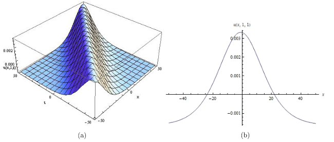
Fig. 1. The 3D and corresponding 2D solution graphs of solitary wave soliton solution for Eq. (5.30) with ${{\beta }_{1}}=0.1$, ${{\beta }_{2}}=0.1$, ${{\beta }_{3}}=0.1$, ${{\wp }_{1}}(t)=1$, ${{\wp }_{4}}(t)=1$, ${{\wp }_{5}}(t)=1$, ${{\wp }_{6}}(t)=1$ and $y=1$. |
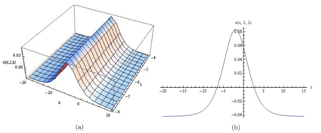
Fig. 2. The 3D and corresponding 2D solution graphs of solitary wave soliton solution for Eq. (5.31) with ${{\beta }_{1}}=0.01$, ${{\beta }_{2}}=0.5$, ${{\beta }_{3}}=1$, ${{\wp }_{1}}(t)=1$, ${{\wp }_{4}}(t)=1$, ${{\wp }_{5}}(t)=1$, ${{\wp }_{6}}(t)={{e}^{t}}$ and y=1. |

Fig. 3. The 3D and corresponding 2D solution graphs of solitary wave soliton solution for Eq. (5.32) with ${{\beta }_{1}}=1$, ${{\beta }_{2}}=1$, ${{\beta }_{3}}=1$, ${{\wp }_{1}}(t)=1$, ${{\wp }_{4}}(t)=1$, ${{\wp }_{5}}(t)=1$, ${{\wp }_{6}}(t)=\sin (t)$ and y=1. |
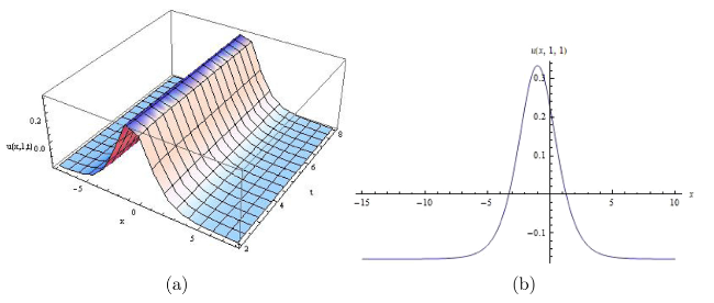
Fig. 4. The 3D and corresponding 2D solution graphs of solitary wave soliton solution for Eq. (5.33) with ${{\beta }_{1}}=-1.5$, ${{\beta }_{2}}=1$, ${{\beta }_{3}}=1.001$, ${{\wp }_{1}}(t)={{e}^{t}}$, ${{\wp }_{4}}(t)=1$, ${{\wp }_{5}}(t)=1$, ${{\wp }_{6}}(t)=\sin (t)$ and y=1. |
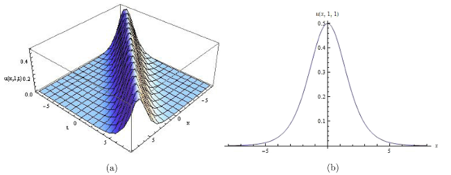
Fig. 5. The 3D and corresponding 2D solution graphs of solitary wave soliton solution for Eq. (5.49) with ${{\beta }_{1}}=1$, ${{\beta }_{2}}=1$, ${{\wp }_{1}}(t)=1$, ${{\wp }_{2}}(t)=1$, ${{\wp }_{3}}(t)=1$, ${{\wp }_{4}}(t)=1$, ${{\wp }_{5}}(t)=1$, ${{\wp }_{6}}(t)=1$, ${{\wp }_{7}}(t)=1$ and y=1. |
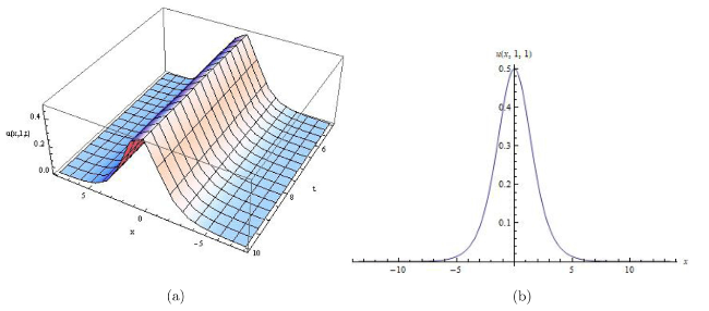
Fig. 6. The 3D and corresponding 2D solution graphs of solitary wave soliton solution for Eq. (5.50) with ${{\beta }_{1}}=1$, ${{\beta }_{2}}=1$, ${{\wp }_{1}}(t)={{e}^{t}}$, ${{\wp }_{2}}(t)=1$, ${{\wp }_{3}}(t)=1$, ${{\wp }_{4}}(t)=1$, ${{\wp }_{5}}(t)=1$, ${{\wp }_{6}}(t)=1$, ${{\wp }_{7}}(t)=1$ and y=1. |
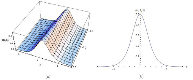
Fig. 7. The 3D and corresponding 2D solution graphs of solitary wave soliton solution for Eq. (5.51) with ${{\beta }_{1}}=1$, ${{\beta }_{2}}=1$, ${{\wp }_{1}}(t)=1$, ${{\wp }_{2}}(t)=\sin (t)$, ${{\wp }_{3}}(t)=1$, ${{\wp }_{4}}(t)=1$, ${{\wp }_{5}}(t)=1$, ${{\wp }_{6}}(t)=1$, ${{\wp }_{7}}(t)=t$ and y=1. |
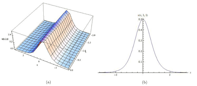
Fig. 8. The 3D and corresponding 2D solution graphs of solitary wave soliton solution for Eq. (5.52) with ${{\beta }_{1}}=1$, ${{\beta }_{2}}=1$, ${{\wp }_{1}}(t)=1$, ${{\wp }_{2}}(t)=\sin (t)$, ${{\wp }_{3}}(t)=1$, ${{\wp }_{4}}(t)=1$, ${{\wp }_{5}}(t)=1$, ${{\wp }_{6}}(t)=1$, ${{\wp }_{7}}(t)=\cos (t)$ and y=1. |
As an outcome, the results are depicted graphically to demonstrate the physical phenomena of time dependent variable coefficients in the (2+1)-dimensional extended Sakovich equation. It is worth mentioning that changing the free parameters ${{\beta }_{1}}$, ${{\beta }_{2}}$, ${{\beta }_{3}}$ and taking different values of functions ${{\wp }_{1}}(t)$, ${{\wp }_{2}}(t)$, ${{\wp }_{3}}(t)$, ${{\wp }_{4}}(t)$, ${{\wp }_{5}}(t)$, ${{\wp }_{6}}(t)$, ${{\wp }_{7}}(t)$ would illustrate various different dynamics of solitary soliton wave structures for Eq. (1.4).
The 3D and corresponding 2D solution graphs of Eq. (1.5) are given as:
Fig. 9 depicts a solitary wave soliton solution with ${{\beta }_{1}}=1$, ${{\beta }_{2}}=1$, ${{\beta }_{3}}=1$ and ${{\wp }_{1}}(t)=1$, ${{\wp }_{4}}(t)=1$, ${{\wp }_{5}}(t)=1$, ${{\wp }_{6}}(t)=1$ for Eq. (6.30). However Fig. 10 presented the same with ${{\beta }_{1}}=1$, ${{\beta }_{2}}=1$, ${{\beta }_{3}}=1$ and ${{\wp }_{1}}(t)={{e}^{t}}$, ${{\wp }_{4}}(t)=1$, ${{\wp }_{5}}(t)=1$, ${{\wp }_{6}}(t)=1$ for Eq. (6.31). Again a solitary wave soliton solution is being observed with ${{\beta }_{1}}=2$, ${{\beta }_{2}}=2$, ${{\beta }_{3}}=2$ and ${{\wp }_{1}}(t)=1$, ${{\wp }_{4}}(t)=1$, ${{\wp }_{5}}(t)=1$, ${{\wp }_{6}}(t)=t$ for Eq. (6.32) in Fig. 11, while Fig. 12 depicts the same observation with ${{\beta }_{1}}=1$, ${{\beta }_{2}}=2$, ${{\beta }_{3}}=1$ and ${{\wp }_{1}}(t)=1$, ${{\wp }_{4}}(t)=1$, ${{\wp }_{5}}(t)=1$, ${{\wp }_{6}}(t)=\cos (t)$ for Eq. (6.33). Fig. 13 reveals a solitary wave with ${{\beta }_{1}}=1$, ${{\beta }_{2}}=1$ and ${{\wp }_{1}}(t)=1$, ${{\wp }_{2}}(t)=1$, ${{\wp }_{3}}(t)=1$, ${{\wp }_{4}}(t)=1$, ${{\wp }_{5}}(t)=1$, ${{\wp }_{6}}(t)=1$, ${{\wp }_{7}}(t)=1$, ${{\wp }_{8}}(t)=1$, ${{\wp }_{9}}(t)=1$, s(t)=1 for Eq. (6.49). The same is being observed with${{\beta }_{1}}=1$, ${{\beta }_{2}}=1$ and ${{\wp }_{1}}(t)={{e}^{t}}$, ${{\wp }_{2}}(t)=1$, ${{\wp }_{3}}(t)=1$, ${{\wp }_{4}}(t)=1$, ${{\wp }_{5}}(t)=1$, ${{\wp }_{6}}(t)=1$, ${{\wp }_{7}}(t)=1$, ${{\wp }_{8}}(t)=1$, ${{\wp }_{9}}(t)=1$, s(t)=1 for Eq. (6.50) in Fig. 14. Again Fig. 15 discloses a solitary wave with ${{\beta }_{1}}=1$, ${{\beta }_{2}}=1$ and ${{\wp }_{1}}(t)=1$, ${{\wp }_{2}}(t)=1$, ${{\wp }_{3}}(t)=1$, ${{\wp }_{4}}(t)=1$, ${{\wp }_{5}}(t)=1$, ${{\wp }_{6}}(t)=1$, ${{\wp }_{7}}(t)=\cos (t)$, ${{\wp }_{8}}(t)=1$, ${{\wp }_{9}}(t)=1$, s(t)=sin(t) for Eq. (6.51). However, the same has been seen with ${{\beta }_{1}}=1$, ${{\beta }_{2}}=1$ and ${{\wp }_{1}}(t)={{e}^{t}}$, ${{\wp }_{2}}(t)=1$, ${{\wp }_{3}}(t)=1$, ${{\wp }_{4}}(t)=1$, ${{\wp }_{5}}(t)=1$, ${{\wp }_{6}}(t)=\sin (t)$, ${{\wp }_{7}}(t)=\cos (t)$, ${{\wp }_{8}}(t)=1$, ${{\wp }_{9}}(t)=1$, s(t)=t for Eq. (6.52) in Fig. 16.
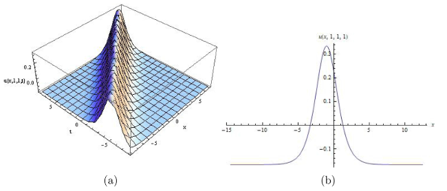
Fig. 9. The 3D and corresponding 2D solution graphs of solitary wave soliton solution for Eq. (6.30) with ${{\beta }_{1}}=1$, ${{\beta }_{2}}=1$, ${{\beta }_{3}}=1$, ${{\wp }_{1}}(t)=1$, ${{\wp }_{4}}(t)=1$, ${{\wp }_{5}}(t)=1$, ${{\wp }_{6}}(t)=1$ and y=1, z=1. |
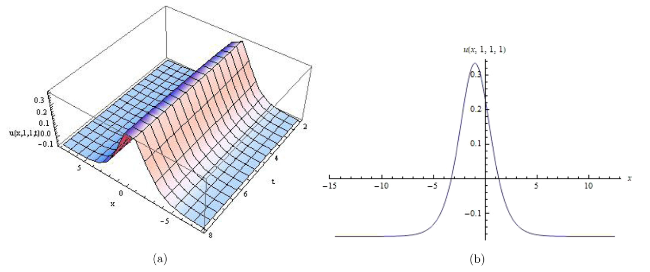
Fig. 10. The 3D and corresponding 2D solution graphs of solitary wave soliton solution for Eq. (6.31) with ${{\beta }_{1}}=1$, ${{\beta }_{2}}=1$, ${{\beta }_{3}}=1$, ${{\wp }_{1}}(t)={{e}^{t}}$, ${{\wp }_{4}}(t)=1$, ${{\wp }_{5}}(t)=1$, ${{\wp }_{6}}(t)=1$ and y=1, z=1. |
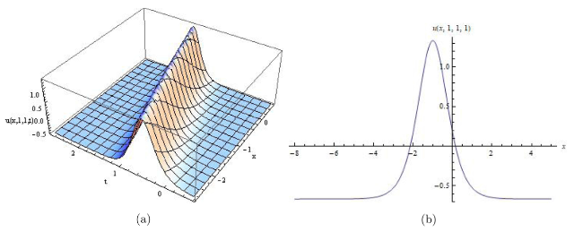
Fig. 11. The 3D and corresponding 2D solution graphs of solitary wave soliton solution for Eq. (6.32) with ${{\beta }_{1}}=2$, ${{\beta }_{2}}=2$, ${{\beta }_{3}}=2$, ${{\wp }_{1}}(t)=1$, ${{\wp }_{4}}(t)=1$, ${{\wp }_{5}}(t)=1$, ${{\wp }_{6}}(t)=t$ and y=1, z=1. |
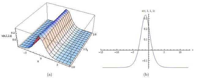
Fig. 12. The 3D and corresponding 2D solution graphs of solitary wave soliton solution for Eq. (6.33) with ${{\beta }_{1}}=1$, ${{\beta }_{2}}=1$, ${{\beta }_{3}}=1$, ${{\wp }_{1}}(t)=1$, ${{\wp }_{4}}(t)=1$, ${{\wp }_{5}}(t)=1$, ${{\wp }_{6}}(t)=\cos (t)$ and y=1, z=1. |
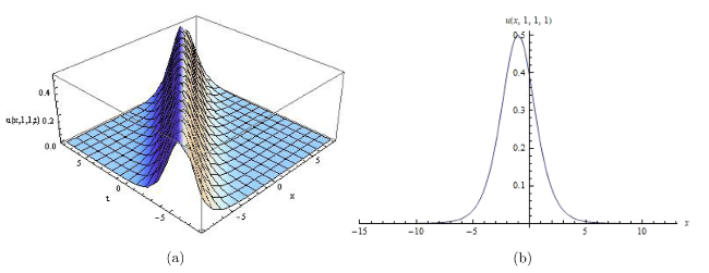
Fig. 13. The 3D and corresponding 2D solution graphs of solitary wave soliton solution for Eq. (6.49) with ${{\beta }_{1}}=1$, ${{\beta }_{2}}=1$, ${{\wp }_{1}}(t)=1$, ${{\wp }_{2}}(t)=1$, ${{\wp }_{3}}(t)=1$, ${{\wp }_{4}}(t)=1$, ${{\wp }_{5}}(t)=1$, ${{\wp }_{6}}(t)=1$, ${{\wp }_{7}}(t)=1$, ${{\wp }_{8}}(t)=1$, ${{\wp }_{9}}(t)=1$, s(t)=1 and y=1, z=1. |

Fig. 14. The 3D and corresponding 2D solution graphs of solitary wave soliton solution for Eq. (6.50) with ${{\beta }_{1}}=1$, ${{\beta }_{2}}=1$, ${{\wp }_{1}}(t)={{e}^{t}}$, ${{\wp }_{2}}(t)=1$, ${{\wp }_{3}}(t)=1$, ${{\wp }_{4}}(t)=1$, ${{\wp }_{5}}(t)=1$, ${{\wp }_{6}}(t)=1$, ${{\wp }_{7}}(t)=1$, ${{\wp }_{8}}(t)=1$, ${{\wp }_{9}}(t)=1$, s(t)=1 and y=1, z=1. |
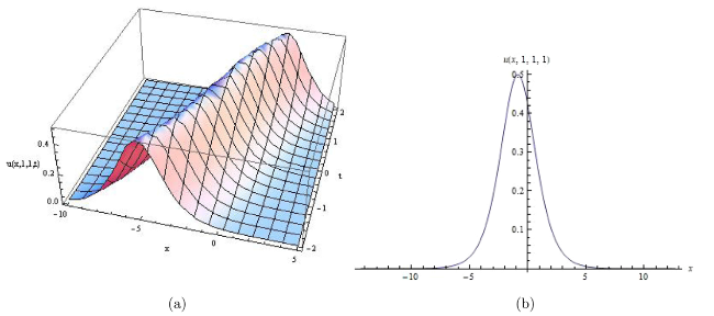
Fig. 15. The 3D and corresponding 2D solution graphs of solitary wave soliton solution for Eq. (6.51) with ${{\beta }_{1}}=1$, ${{\beta }_{2}}=1$, ${{\wp }_{1}}(t)=1$, ${{\wp }_{2}}(t)=1$, ${{\wp }_{3}}(t)=1$, ${{\wp }_{4}}(t)=1$, ${{\wp }_{5}}(t)=1$, ${{\wp }_{6}}(t)=1$, ${{\wp }_{7}}(t)=\cos (t)$, ${{\wp }_{8}}(t)=1$, ${{\wp }_{9}}(t)=1$, s(t)=sin(t) and y=1, z=1. |
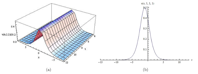
Fig. 16. The 3D and corresponding 2D solution graphs of solitary wave soliton solution for Eq. (6.52) with ${{\beta }_{1}}=1$, ${{\beta }_{2}}=1$, ${{\wp }_{1}}(t)={{e}^{t}}$, ${{\wp }_{2}}(t)=1$, ${{\wp }_{3}}(t)=1$, ${{\wp }_{4}}(t)=1$, ${{\wp }_{5}}(t)=1$, ${{\wp }_{6}}(t)=\sin (t)$, ${{\wp }_{7}}(t)=\cos (t)$, ${{\wp }_{8}}(t)=1$, ${{\wp }_{9}}(t)=1$, s(t)=t and y=1, z=1. |
As an outcome, the results are depicted graphically to demonstrate the physical phenomena of time dependent variable coefficients in the (3+1)-dimensional extended Sakovich equation.
It is worth mentioning that changing the free parameters ${{\beta }_{1}}$, ${{\beta }_{2}}$, ${{\beta }_{3}}$ and taking different values of functions ${{\wp }_{1}}(t)$, ${{\wp }_{2}}(t)$, ${{\wp }_{3}}(t)$, ${{\wp }_{4}}(t)$, ${{\wp }_{5}}(t)$, ${{\wp }_{6}}(t)$, ${{\wp }_{7}}(t)$, ${{\wp }_{8}}(t)$, ${{\wp }_{9}}(t)$, s(t) would illustrate various different dynamics of solitary soliton wave structures for Eq. (1.5).
8. Conclusion
This article introduced the Painlevé analysis and ABT for (2+1) and (3+1)-dimensional extended variable coefficients Sakovich Eqs. (1.4) and (1.5). Painlevé analysis is employed to test the integrability of Eqs. (1.4) and (1.5) while an ABT is used to derive family of new exact soliton solutions for Eqs. (1.4) and (1.5). Truncated Painlevé expansion An ABT for each of the Eqs. (1.4) and (1.5) is derived by truncating the Laurent series given by Eqs. (3.5) and (4.3) respectively. Families of two exact analytical solutions have obtained for each of the equations. The analytic solutions are obtained in the form of rational and exponential functions. To understand the physical behaviour of the considered equations, solutions are also graphically illustrated. New solitary wave soliton solutions are explored, which can be viewed as 3D and 2D graphs presented in this article. For determining the exact solutions of NLPDEs, the ABT approach is more effective, simple and straightforward to utilise.
Author contribution statement
Both the authors contributed equally to this work.
Data availability
The datasets generated during and/or analysed during the current study are available from the corresponding author on reasonable request.
Declaration of Competing Interest
Authors declare that they have no conflict of interest.
