
1. Introduction
Accurate prediction of ships' underwater radiated noise is vital to further enhance target detection and improve the ocean acoustic environment [1], [2], [3]. As a complex elastic structure on water, ships will be subjected to various excitations and generate vibration and mechanical noise, which could damage the marine ecological balance. Underwater radiated noise emitted by ships has dominated the marine background noise in low frequencies [4]. The marine noise level generated by ships is still increasing by 0.2 dB per year [5,6], and adversely interfered with the daily life of marine creatures, including hunting, breeding, avoiding predators, and navigating [7], [8], [9]. Besides the protection of marine life, the underwater radiated noise level is the most important indicator to evaluate the acoustic stealth performance of a warship. Decreasing radiated noise could effectively reduce ships’ risk of being detected, and improve their survival and combat capability [10]. Therefore, military equipment must meet stricter requirements for noise control with the development of sonar technology [10,11]. As the most important component of ships’ underwater radiated noise in low frequencies, if mechanical noise can be accurately predicted at the design stage, it will provide the basis for the subsequent control of vibration and noise.
Simulation and experiment are the two main ways to obtain the ships’ mechanical noise. During the past few decades, various methods have been developed to obtain structures' acoustic radiated and hydroacoustic experiments [12]. On the one hand, as an indicator of acoustic prediction, the hydroacoustic measurement is the basis of simulated analysis. Hydroacoustic experiments could be generally classified into the single hydrophone system [13], horizontal hydrophone array system [14], vertical line hydrophone array system [15], hydrophone cluster system [16], and vector hydrophone system [17]. Some critical issues are discussed in hydroacoustic experiments, including the free surface interference and waveguide [18], [19]. On the other hand, the simulated results largely depend on the calculation model and the loading method. Appropriate for the large-scale structures with complex shapes, the simulated approaches of ships’ mechanical noise include the FEM or BEM performed in low frequencies [20], [21], [22] and the SEA adopted in high frequencies [23]. Based on the acoustic FEM to predict the vibroacoustic behavior of a ship, the structure and the fluid both need to be modeled with finite elements [21], and the acoustic absorbing boundary condition is set at the edge of the fluid field. The acoustic BEM method is discrete structures into finite elements, and the fluid field is simulated by boundary elements on the wetted surface [24]. The acoustic BEM is recommended to calculate ships' radiated noise with higher precision and effectiveness [22,25].
The loading method of mechanical equipment has a direct impact on the simulated result. In engineering, the forms of equipment excitation include forces and moments, power flows, and acceleration loads. However, limited by measurement methods and installation conditions, the generalized force and the power flow of mechanical equipment are generally difficult to measure, especially the moments [26]. The response acceleration can be easily obtained. Therefore, the acceleration load is regarded as the most practical way to characterize the excitation of equipment and calculate structural vibration and acoustic radiation.
Directly using acceleration load, there still exist some problems for predicting a ship's mechanical noise [27]. Firstly, sometimes it is difficult to directly obtain the acceleration load in the design stage. Alternatively, the acceleration cannot be measured due to the complicated installation condition. Loads of bench testing are provided, but cannot be used directly to calculate the vibration and noise of a real ship, because of the different support foundations. Secondly, there are numerous connection points between larger-scale equipment and base panel, which make it impossible to measure the acceleration response of all connection points. The average acceleration of several typical connection points could be measured to characterize the equipment load. Finally, even if it is possible to measure the response acceleration of all connection points, there is a phase difference between the different acceleration responses. The phase difference affects structural vibration and radiated noise, and the quantitative correction of the phase difference on the radiated noise prediction result still needs further investigation [28].
In the paper, the loading method of mechanical equipment is further investigated, which is divided into three criteria depending on different types of acceleration loads. Firstly, the effects of acceleration amplitude distribution and phase information on mechanical noise are detail investigated, and an" equipment-isolator-base-hull" coupled dynamic model is established. The analytical formulas are theoretically derived from structural dynamics to achieve equivalent conversion between generalized forces and ideal accelerations [29,30], constituting the first criterion. Subsequently, to deal with the absence of phase and amplitude distribution, three load models are proposed to calculate the vibroacoustic transfer function, which can determine the upper and lower limits of underwater radiated sound power together with the average acceleration load, and energy-averaged value is used to represent ships’ mechanical noise in the second criterion. Furthermore, the third load criterion is used to handle load conversion between the bench testing and the real ship, and predict mechanical noise of ships. Finally, three parameters such as overall level error, correlation coefficient, and standard deviation are used to quantitatively evaluate the computational accuracy, and the load criteria are verified by the model experiments.
2. The influence of acceleration loads on mechanical noise
The connection between a base panel and mechanical equipment is often complicated, and there are many connection points. Sometimes, it is difficult and costly to accurately measure all connection points' acceleration. The average is used to characterize the equipment excitation in engineering. The ideal acceleration includes the phase information, amplitude distribution, and the number of connection points, while it is hard to be met. A ship's scale model is taken as an example to investigate the influence of acceleration parameters on mechanical noise.
2.1. Numerical model
The numerical model is also the experimental model. The length of the experimental model is 11.2 m, and the width is 5.6 m. The draft is 1.2 m, and the depth is 3.6 m. The displacement is nearly 48.5t, and the material is Q235 steel. The experimental model retained the typical structural form of a ship, which included single bottom, double bottom, ballast water tank, deck, and some bases. In the modeling process, plate structures are simulated by quadrilateral and triangular shell elements. The cross-beams, longitudinal frames, and stiffeners are simulated by beam elements with offsets. The mechanical equipment is simulated by mass elements and is placed in the corresponding installation location. Solid elements are used to simulate ballast water in fluid tanks. The elements’ size meets the principle that one wavelength contains six elements at least [31]. In this paper, the underwater radiated sound power is obtained by the acoustic boundary element method [24,32,33], as shown in Fig. 1.
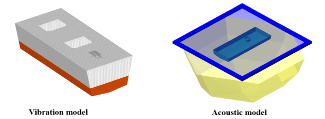
Fig. 1. The vibration and acoustic calculation model. |
Acceleration levels, sound power levels, and its integration formulas in the engineering are shown below:
$LA=20\log \left( a/{{a}_{0}} \right)$
$OLA=10\log \left( \underset{f={{f}_{1}}}{\overset{f={{f}_{2}}}{\mathop \sum }}\,{{10}^{\frac{L{{A}_{f}}}{10}}} \right)$
$Lw=10\log \left( {{P}_{w}}/{{P}_{w}}_{0} \right)$
$OLw=10\log \left( \underset{f={{f}_{2}}}{\overset{f={{f}_{1}}}{\mathop \sum }}\,{{10}^{\frac{L{{w}_{f}}}{10}}} \right)$
where, LA is the acceleration level, dB; a is the response acceleration, m/s2; a0 is the reference acceleration that equals 10-6 m/s2. OLA is the integrated acceleration level, dB; f1 is the lower frequency, Hz; f2 is the upper frequency, Hz. Lw is the sound power level, dB; Pw is the radiated sound power, W; P0 is the reference sound power that equals 10-12 W. OLw is the integrated sound power level, dB.
2.2. Effects of acceleration components on mechanical noise
The response acceleration of the base panel caused by mechanical equipment can be decomposed as Ax, Ay, and Az in the spatial Cartesian coordinate system (Oxyz), respectively. The sound power of the model under three acceleration load conditions is calculated from 20 Hz to 1000 Hz. The load model is shown in Fig. 2, and the results are shown in Fig. 3. The load cases Ax, Ay, and Az indicate that the model is subjected to unit acceleration components in the x-directional, y-directional, and z-directional, respectively.
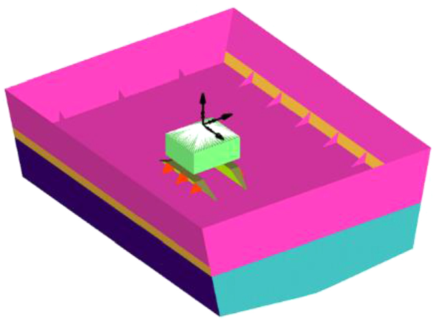
Fig. 2. The load model. |

Fig. 3. The sound power under acceleration load conditions. |
As shown in Fig. 3, the overall sound power level of load case Az is 17 dB much larger than those of load case Ax and load case Ay. It can be seen from Fig. 4 that the underwater radiated noise energy caused by the acceleration component Az is much larger than those caused by the acceleration components Ax and Ay under the same amplitude. Therefore, when mechanical noise needs to be predicted by the acceleration load, only Az terms are included and the other components (Ax and Ay) can be neglected.
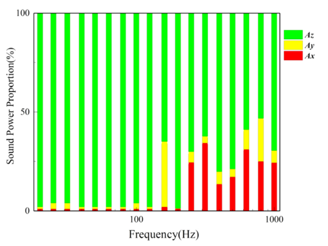
Fig. 4. Energy proportional distribution caused by the acceleration components. |
2.3. Effects of acceleration phase on mechanical noise
The model is assumed that the generalized forces are applied in the frequency band, including Fx=13 N, Fy=16 N, Fz=8 N, Mx=75Nm, My=86Nm, Mz=178Nm. According to vibration results, the response acceleration of the base panel is output, and the acceleration is used as the excitation to calculate the sound power again. The acceleration load is divided into two load conditions. (1) Load case Az indicates that the acceleration load only includes the amplitude information. (2) Load case AP denotes that the acceleration load includes both amplitude and phase information. The underwater radiated sound power curves under two acceleration load conditions are compared with the results generated by the generalized forces, as shown in Fig. 5.
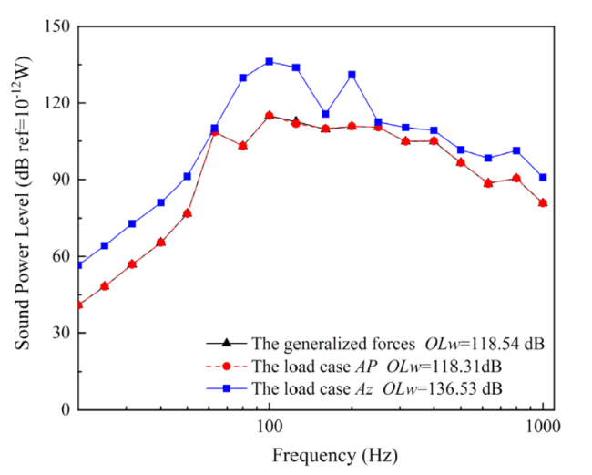
Fig. 5. The gradient meshing model of the experimental model. |
As shown in Fig. 5, compared with the results of the generalized forces load case, the error is only 0.21 dB in the case where the acceleration loads include the amplitude and phase information, while the error reaches17.99 dB in the case where the acceleration loads only include the amplitude. It is found that the precision is higher with considering the amplitude and phase information, while the error is larger only considering the amplitude. It results from a phase difference in the response acceleration of connection points, and the structural vibration and mechanical noise are related to not only the amplitude but also the phase information.
2.4. Effects of the acceleration amplitude distribution
According to the response acceleration under the generalized forces, the amplitude of the acceleration load is averaged. Then, the average acceleration is applied to the model, and the phase of each connection point is guaranteed to be unchanged. Underwater radiated sound power level under the average acceleration with phase information is calculated, as shown in Fig. 6.
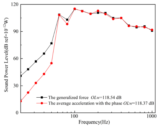
Fig. 6. The effect of acceleration amplitude distribution on underwater radiated noise. |
In Fig. 6, it can be observed that the overall sound power levels of these load cases (the average acceleration with the phase and the generalized force) are 118.37 dB and 118.54 dB, respectively, and the error is only 0.17 dB. Comparing the two sound power curves, there are some differences in the low-frequency domain. However, as the frequency increases, the trends of the sound power curve are identical. The peak frequencies and peak numbers are consistent. Therefore, the loading method with an average acceleration considering the phase is sufficiently accurate in engineering.
3. The load criteria of ships’ mechanical excitations
The forms of equipment excitation include forces and moments, power flows, and acceleration loads. The forces and moments are defined as the standard form. Power flows and acceleration loads must be converted into generalized forces. This is because generalized force can be used for calculating a ship's mechanical noise in full frequencies, while power flow is difficult to use in low frequencies and acceleration load results in large errors in high frequencies. In addition, the generalized force of mechanical equipment is constant [34], while the power flows and the acceleration load will change with the different supporting foundations [26].
3.1. The underwater radiation sound field under standard load
The vibration system is defined in a space Cartesian coordinate system, with the X-axis pointing towards the bow, Z-axis pointing the upwards. The ship's structure is assumed to be linear and time-independent, with a small deformation in the equilibrium position. The damping is simplified to Rayleigh damping. The differential equation of vibration is as follows:
$\mathbf{M\ddot{X}}+\mathbf{C\dot{X}}+\mathbf{KX}=\mathbf{F}$
where M, C, and K are matrices of generalized mass, generalized damping, and generalized stiffness. X is a column vector. F is generalized forces.
$\begin{matrix} \mathbf{\dot{X}}=j\omega \mathbf{X} \\ \mathbf{\dot{X}}=\frac{1}{j\omega }\mathbf{\ddot{X}} \\ \end{matrix}$
Considering the coupling between structure and fluid, the dynamic equations can be obtained by substituting Eq. (6) into Eq. (5),
$\left( j\omega \mathbf{M}+\mathbf{C}-\frac{j}{\omega }\mathbf{K} \right)\mathbf{\dot{X}}=\mathbf{F}+{{\mathbf{p}}_{s}}$
where, $\omega $ is the circular frequency, and j2=−1; ${{\mathbf{p}}_{s}}$ is sound pressure in coupling surface.
The radiated sound pressure generated by a structural vibration in water satisfies the Helmholtz equation and Sommerfeld radiated condition [21],
${{\nabla }^{2}}p\left( {\vec{r}} \right)+{{k}^{2}}p\left( {\vec{r}} \right)=0$
$\frac{\partial p\left( {\vec{r}} \right)}{\partial \vec{n}}=i\omega \rho {{v}_{n}}$
where, $\vec{n}$ is the unit vector of exterior normal of the wetted surface S, and ${{v}_{n}}$ is the normal vibration velocity of the wetted surface S. $\rho $ is the density of the fluid. k is the wavenumber. $\vec{r}$ is the vector at the reception point.
According to the acoustic boundary element method, the sound pressure at any reception point can be obtained [35],
$p\left( {\vec{r}} \right)={{\mathbf{H}}_{AF}}\mathbf{F}$
where,
${{\mathbf{H}}_{AF}}=\left( {{\mathbf{B}}^{T}}\mathbf{Z}+{{\mathbf{R}}^{T}} \right){{\left( \left( j\omega \mathbf{M}+\mathbf{C}-\frac{j}{\omega }\mathbf{K} \right)\mathbf{N}-\mathbf{Z} \right)}^{-1}}$
${{\mathbf{H}}_{AF}}$ is a row vector, which can be treated as a transfer vector of sound pressure resulting from the exciting force. $\mathbf{B}$ and $\mathbf{R}$ are matrices associated with the reception point $\vec{r}$. $\mathbf{Z}$ is surface sound radiated impedance matrix which is only subject to the geometry of the structural surface, the numerical discretization, and the frequency of excitation. $\mathbf{N}$ is the transfer matrix that can convert the vector of vibration velocity into the normal vector of vibration velocity.
While it is challenging to accurately measure generalized forces of mechanical equipment under various working conditions in engineering, the response acceleration of the base panel can be easily obtained, and often used to characterize the excitation of equipment. However, directly using acceleration load neglecting phase information to predict the mechanical noise, the error is large. This section proposes three criteria for load transformation according to three different types of acceleration loads to predict the ship's mechanical noise precisely.
3.2. The first load criterion
Based on the fundamental equations of structural dynamics, equivalent formulas establish the first load criterion between ideal accelerations and generalized forces. The mechanical equipment is installed on a base with some isolators, which constitutes a force transfer system. Since the stiffness of mechanical equipment is much greater than that of the "isolator-base" system, the equipment can be considered as a rigid body. According to theoretical mechanics, the generalized forces generated by mechanical equipment can be equivalent to a combined force and moment, as shown in Fig. 7(a). Assuming that exciting forces are only transferred through the connection points, the input loads are equated to the excitation at the connection points, and the mechanical model of the system is shown in Fig. 7(b).

Fig. 7. The mechanical model of the equipment and base system. |
Rewriting the Eq. (5),
$\left( \mathbf{M}+\frac{1}{j\omega }\mathbf{C}-\frac{1}{{{\omega }^{2}}}\mathbf{K} \right)\mathbf{\ddot{X}}=\mathbf{F}$
Assuming the number of connection points is n, response accelerations and generalized forces are decomposed in a spatial Cartesian coordinate system. The base panel is excited by ${{F}_{1}}_{x}$, ${{F}_{1}}_{y}$, ${{F}_{1}}_{z}$, ${{F}_{2x}}$, ${{F}_{2y}}$, ${{F}_{2z}}$,⋯ ${{F}_{nx}}$, ${{F}_{ny}}$, ${{F}_{nz}}$, as shown in Fig. 7(b), and the response accelerations of the base panel are ${{a}_{1x}}$, ${{a}_{1y}}$, ${{a}_{1z}}$, ${{a}_{2x}}$, ${{a}_{2y}}$, ${{a}_{2z}}$,⋯, ${{a}_{nx}}$, ${{a}_{ny}}$, ${{a}_{nz}}$. The dynamic equation can be obtained,
${{\mathbf{F}}_{3n}}=\mathbf{H}_{3n\times 3n}^{-1}{{\mathbf{a}}_{3n}}$
where ${{\mathbf{H}}_{3n\times 3n}}$ is the transfer function matrices; ${{\mathbf{a}}_{3n}}$ is a column vector of response acceleration; ${{\mathbf{F}}_{3n}}$ is a column vector of generalized force.
By Eq. (13), the conversion between generalized force and response acceleration can be achieved, and the generalized forces can be obtained by load identification methods [36,37]. In the process of load identification, it is inevitable to encounter the problem of ill-condition transfer matrices [29,30,38]. Therefore, a total least squares regularization algorithm is introduced to load identification methods to reduce the condition number of matrices and improve the precision of the identification [39]. It should be noted that the response acceleration and transfer function in Eq. (13) both include amplitude and phase information.
Eq. (13) shows that an equivalent conversion is achieved between the response accelerations and the generalized forces, and the radiated acoustic field can be obtained by substituting Eq. (13) into Eq. (10), which constitute the first load criterion. The hull vibration and radiated noise which are predicted by the identified forces agree well with that generated by the excitation of mechanical equipment.
3.3. The second load criterion
For large-scale mechanical equipment, the excitation is usually characterized by the average acceleration in engineering. It is impossible to determine the amplitude distribution and phase information by average acceleration, which cannot obtain the correct forces with load identification. Therefore, to address the issue that the acceleration load information is absent, the loading method is proposed based on the load model. The upper and lower limits of sound power are determined by a vibroacoustic transfer function, and the energy-averaged value is characterized by mechanical noise. A method for calculating mechanical noise based on the second load criterion is given, first to illustrate vibroacoustic transfer function based on acceleration and second to provide insight into the vibroacoustic behavior of structures with different generalized forces. Lastly, based on the vibroacoustic transfer function of the single-point excitation and the load model, multipoint acceleration excitations are transformed into single-point exciting force or moment by different load models to determine the range of underwater radiated sound power and the energy-averaged value.
3.3.1. The vibroacoustic transfer function based on acceleration load
The basis of the formulation is that the effects of forces and moments on underwater radiated noise can be compared in terms of intermediate quantity. According to the theory of vibration and acoustics, the vibroacoustic transfer function based on the acceleration of the base panel is first established under single source excitation. The significance of forces and moments on underwater radiated noise is directly compared via the vibroacoustic transfer function. According to the structural dynamics’ theory, the vibration velocity at any point of the structure obtained by modal superposition is,
${{v}_{l}}\left( \omega \right)=\underset{r=1}{\overset{N}{\mathop \sum }}\,\frac{\omega {{\varphi }_{lr}}{{\varphi }_{pr}}{{f}_{p}}}{-{{\omega }^{2}}{{M}_{r}}+j\omega {{C}_{r}}+{{K}_{r}}}$
where Mr is the modal mass; Cr is the modal damping; Kr is the modal stiffness; fp is the modal generalized force; ${{\varphi }_{lr}}$ and ${{\varphi }_{pr}}$ are the modal vector; p is the loading point; l is the arbitrary response point of the structure.
The response acceleration at the loading point is,
${{a}_{p}}\left( \omega \right)=\underset{r=1}{\overset{N}{\mathop \sum }}\,\frac{{{\omega }^{2}}{{\varphi }_{pr}}^{2}{{f}_{p}}\left( \omega \right)}{-{{\omega }^{2}}{{M}_{r}}+j\omega {{C}_{r}}+{{K}_{r}}}$
The transfer function between the RMS vibration velocity of the hull's wet surface and the vibration acceleration of the base panel is,
$H_{lp}^{\bar{v}a}\left( \omega \right)=\frac{{\bar{v}}}{\mathop{\sum }_{r=1}^{N}\frac{{{\omega }^{2}}\varphi _{pr}^{2}{{f}_{p}}\left( \omega \right)}{-{{\omega }^{2}}{{M}_{r}}+j\omega {{C}_{r}}+{{K}_{r}}}}$
where,
$\bar{v}=\sqrt{\frac{1}{{{n}_{1}}}\underset{{{n}_{1}}}{\mathop \sum }\,v_{i}^{2}}=\sqrt{\frac{1}{{{n}_{1}}}\left( \underset{{{n}_{1}}}{\mathop \sum }\,{{\left( \underset{{{r}_{1}}=1}{\overset{N}{\mathop \sum }}\,\frac{\omega {{\varphi }_{pr}}{{\varphi }_{lr}}{{f}_{p}}\left( \omega \right)}{-{{\omega }^{2}}{{M}_{{{r}_{1}}}}+j\omega {{C}_{{{r}_{1}}}}+{{K}_{{{r}_{1}}}}} \right)}^{2}} \right)}$
There is a relationship between the velocity of a ship's wet surface and the radiated sound power under the single source excitation.
${{P}_{w}}=\rho cS\eta \langle {{\bar{v}}^{2}}\rangle =\rho cS\eta {{\left| H_{lp}^{\bar{v}a}\bar{a} \right|}^{2}}=\rho cS\eta {{\left( H_{lp}^{\bar{v}a} \right)}^{2}}{{\left( {\bar{a}} \right)}^{2}}$
where Pw is the radiated acoustic power; S is the wet surface of the hull; $\eta $ is the radiated efficiency of the structure; $\bar{v}$ the RMS velocity of the ships’ wet surface; $\rho c$ is the acoustic impedance of the fluid; $\bar{a}$ is the average acceleration of the base panel.
$\begin{matrix} Lw=10\log \frac{{{P}_{w}}}{{{P}_{w}}_{0}}=10\log \left( \frac{\rho cS\sigma {{\left( H_{lp}^{\bar{v}a} \right)}^{2}}{{\left( {\bar{a}} \right)}^{2}}}{{{P}_{w}}_{0}} \right) \\ =10\log \left( \frac{\rho cS\sigma {{\left( H_{lp}^{\bar{v}a} \right)}^{2}}{{\left( {{a}_{0}} \right)}^{2}}}{{{P}_{w}}_{0}} \right)+20\log \left( \frac{{\bar{a}}}{{{a}_{0}}} \right) \\ \end{matrix}$
$Lw=L{{H}_{VA}}+LA$
As shown in Eq. (20), the sound power level (Lw) consists of the vibroacoustic transfer function level (LHVA) and the response acceleration level (LA). The LHVA is related to the natural properties of the hull structure (mass, damping, stiffness, etc.), the size and the shape of the acoustic radiated surface, the location, and the form of the generalized force. For a defined hull structure, other factors have already been determined, and the vibroacoustic transfer function is only related to the form of the generalized force. The connection between the underwater radiated sound power and the acceleration load of the base panel is directly established by the LHVA.
3.3.2. Predicting mechanical noise based on the average acceleration
For the multiple-source excitation, the multiple forces system can be simplified by the load model, as shown in Fig. 7(a). When the excitation is presented in terms of average acceleration, the generalized forces cannot be uniquely determined because of the acceleration missing information. However, the range of ships’ mechanical noise can be determined by the vibroacoustic transfer function of the various load models. The vibroacoustic transfer function of different load models is used to characterize the effect of the equipment excitation characteristics on the mechanical noise. In Section 2, the results indicate that the mechanical noise is dominated by the Az component of acceleration which is mainly determined by the Fz, Mx, and My components of the generalized force. Therefore, three types of load models are analyzed in the section to calculate the vibroacoustic transfer function, in Fig. 8.
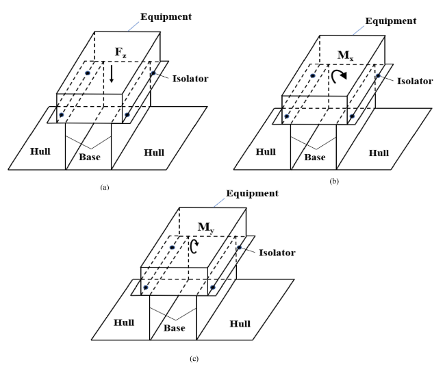
Fig. 8. The equivalent mechanical model of the equipment for the three types of load model. (a) Fz load model;(b) Mx load model; (c)My load model;. |
The load model under the individual component of the generalized force is shown in Fig. 8. Taking the Fz load model as an example, the Eq. (21) can be obtained,
$\bar{a}=\overline{{{H}_{Fz}}}{{F}_{z}}$
where $\bar{a}$ is the average acceleration of the base panel. $\overline{{{H}_{Fz}}}$ is the transfer function under the Fz load model.
Similarly, it can be obtained,
$\bar{a}=\overline{{{H}_{Mx}}}{{M}_{x}}$
$\bar{a}=\overline{{{H}_{My}}}{{M}_{y}}$
where $\overline{{{H}_{Mx}}}$ and $\overline{{{H}_{My}}}$ are the transfer functions under the Mx and the My load model, respectively.
Substituting Eq. (21)-Eq. (23) into Eq. (18), the sound power can be obtained under the individual component of the generalized force,
$\begin{matrix} P_{w}^{Fz}=\rho cS\eta {{\left( H_{Fz}^{\bar{v}a} \right)}^{2}}{{\left( {\bar{a}} \right)}^{2}}=H_{Fz}^{av}{{\left( {\bar{a}} \right)}^{2}} \\ P_{w}^{Mx}=\rho cS\eta {{\left( H_{Mx}^{\bar{v}a} \right)}^{2}}{{\left( {\bar{a}} \right)}^{2}}=H_{Mx}^{av}{{\left( {\bar{a}} \right)}^{2}} \\ P_{w}^{My}=\rho cS\eta {{\left( H_{My}^{\bar{v}a} \right)}^{2}}{{\left( {\bar{a}} \right)}^{2}}=H_{My}^{av}{{\left( {\bar{a}} \right)}^{2}} \\ \end{matrix}$
where $H_{Fz}^{av}$, $H_{Mx}^{av}$ and $H_{My}^{av}$ are the vibroacoustic transfer functions based on average acceleration under the Fz, Mx, and My load model, respectively.
The average acceleration is $\bar{a}$ and we can obtain,
$\bar{a}={{\bar{a}}_{Fz}}+{{\bar{a}}_{Mx}}+{{\bar{a}}_{My}}$
where
$\begin{matrix} {{{\bar{a}}}_{Fz}}=\alpha \bar{a} \\ {{{\bar{a}}}_{Mx}}=\beta \bar{a} \\ {{{\bar{a}}}_{My}}=\alpha \bar{a} \\ \end{matrix}$
${{\bar{a}}_{Fz}}$, ${{\bar{a}}_{Mx}}$ and ${{\bar{a}}_{My}}$ are the average accelerations generated by the Fz, Mx, and My, respectively. $\alpha $, $\beta $ and $\gamma $ are the proportional coefficients, respectively, and it also satisfied,
$\begin{matrix} \alpha +\beta +\gamma =1 \\ 0\le \left( {{\gamma }_{1}},{{\gamma }_{2}},{{\gamma }_{3}} \right)\le 1 \\\end{matrix}$
Chen's [35] research has shown that the sound pressures driven by multiple excitations can be approximated by the energy superposition of individual excitations, as shown in Eq. (27).
${{P}_{w}}\approx P_{w}^{Mx}+P_{w}^{My}+P_{w}^{Fz}=\left( {{\alpha }^{2}}H_{Fz}^{va}+{{\beta }^{2}}H_{Mx}^{va}+{{\gamma }^{2}}H_{My}^{va} \right){{\left( {\bar{a}} \right)}^{2}}$
Assuming,
$\begin{matrix} {{H}_{\min }}=\min \left( H_{Fz}^{va},H_{Mx}^{va},H_{My}^{va} \right) \\ {{H}_{\max }}=\max \left( H_{Fz}^{va},H_{Mx}^{va},H_{My}^{va} \right) \\ \end{matrix}$
Substituting Eq. (28) into Eq. (27), the ranges of sound power can be obtained,
$\frac{1}{3}{{H}_{\min }}{{\left( {\bar{a}} \right)}^{2}}\le {{P}_{w}}\le {{H}_{\max }}{{\left( {\bar{a}} \right)}^{2}}$
In engineering, a defined value is usually used to evaluate whether the design is reasonable or not. In probability problems, the average value is usually used to characterize the final result. the energy-averaged value of sound power can be obtained,
${{P}_{w}}=\frac{P_{w}^{Mx}+P_{w}^{My}+P_{w}^{Fz}}{3}=\frac{\left( H_{Fz}^{va}+H_{Mx}^{va}+H_{My}^{va} \right)}{3}{{\left( {\bar{a}} \right)}^{2}}$
3.4. The third load criterion
The acceleration load obtained from bench tests is often used as the only excitation during the design stage, but it cannot characterize the exciting characteristics of the equipment in practical conditions. The results are also questionable when it is directly applied to calculate the vibration and noise of a ship. Therefore, it is greatly significant to develop a load conversion method between bench test and real installation. Some researches indicate that the conversion method includes free velocity theory [40,41] and load identification [42,43]. In this section, according to the source descriptor invariance assumption, the loading method is proposed to achieve conversion between bench test and real installation, and the mechanical noise also can be predicted simultaneously.
It is also assumed that the mechanical noise is generated by the force Fz and the moments Mx and My. The load model of the acceleration conversion between the bench test and the real ship is shown in Fig. 9. According to source descriptor invariance, the components of the excitation (including Fz, Mx, and Mx) are used as the load model, and the vibration transfer function is used to characterize the dynamic characteristics of the support foundation.
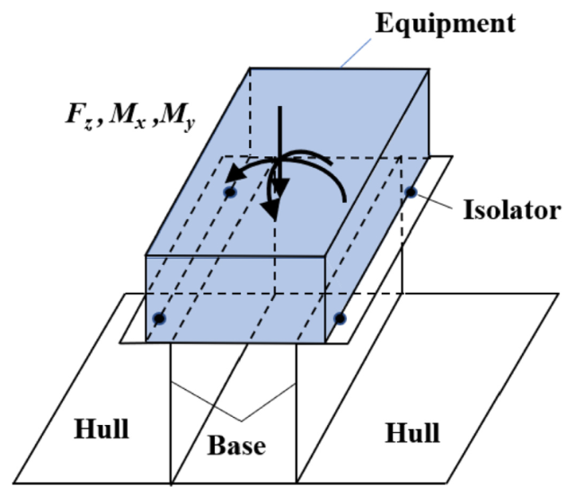
Fig. 9. The mechanical model of load identification. |
The generalized forces of the mechanical equipment can be similarly equivalent to the load model that satisfies a certain proportion between the force and the moment, as well as the acceleration load ratio between the acceleration load of the equipment and the response acceleration under the FzMxy load model. The force and moments satisfy a certain proportionality ${{F}_{z}}:{{M}_{x}}:{{M}_{y}}=1N:aNm:bNm$, and then these excitation components are applied to the structure simultaneously.
For the bench structure, the average acceleration is Abt, and the average transfer function of the bench structure under the FzMxy load model is Hbt. The load ratio Rbt satisfies the following equation,
${{A}_{bt}}={{H}_{bt}}{{R}_{bt}}$
where, Rbt denotes load ratio, which satisfies the particular proportionality ${{F}_{z}}:{{M}_{x}}:{{M}_{y}}={{R}_{bt}}N:a{{R}_{bt}}Nm:b{{R}_{bt}}Nm$. Hbt can be also named as the vibration transfer function based on the FzMxy load model in bench testing.
Similarly, with the same load model and assumptions, the load ratio in a real ship is also satisfied with the following equation,
${{A}_{rs}}={{H}_{rs}}{{R}_{rs}}$
where ${{R}_{rs}}$ denotes load ratio when the equipment is installed on a real ship. ${{A}_{rs}}$ is the acceleration of the base panel, and the ${{H}_{rs}}$ is the transfer function based on the load model in a real ship.
According to the source descriptor invariance, the load model and the load ratio are identical, which satisfies Rrs= Rbt. The acceleration in a real ship satisfies the following equation,
${{A}_{rs}}=\frac{{{H}_{rs}}}{{{H}_{bt}}}{{A}_{bt}}$
According to Eq. (19), the underwater radiated sound power can be obtained as follows.
$Lw=L{{H}_{VA}}+\left( L{{H}_{rs}}-L{{H}_{bt}} \right)+L{{A}_{bt}}$
Eq. (34) achieves predicting mechanical noise based on acceleration loads obtained by bench tests. The coefficients a and b can be determined by the testing or working principle of the equipment.
However, some simplifications are performed in a numerical model of ships, and an offset of the natural frequency will inevitably occur between a numerical model and real structure, resulting in incorrect transfer functions and affecting the accuracy of the acceleration conversion. Additionally, acceleration loads are usually provided in the form of 1/3 octave spectrum, and impossibly determine amplitude distribution in the frequency domain. An energy equivalent method is developed to address the issue.
Assuming that generalized forces of mechanical equipment are uniformly distributed in the given frequency band, it can be obtained,
$\frac{\sum {{A}_{rs}}^{2}}{\sum {{H}_{rs}}^{2}}=\frac{\sum {{A}_{bt}}^{2}}{\sum {{H}_{bt}}^{2}}$
$OLw=OL{{H}_{VA}}+L\bar{A}$
where,
$L\bar{A}=10\text{log}\left( \frac{\sum {{A}_{bt}}^{2}}{\sum {{H}_{bt}}^{2}}\sum H_{rs}^{2} \right)-20\log {{a}_{0}}-20\log {{n}_{f}}$
${{n}_{f}}$ is the frequency bandwidth. $OLw$ is the integrated sound power level in the given frequency band. $OL{{H}_{VA}}$ is the integrated vibroacoustic transfer function level. $L\bar{A}$ is the energy equivalent acceleration level in the given frequency band.
The presented method can reduce computational errors resulting from an offset of the natural frequency, incomplete information of acceleration loads, and pathological matrix.
4. Experimental validation
To validate the three load criteria proposed in the paper for predicting mechanical noise with the acceleration load, the vibration response and underwater acoustic experiments were carried out in Zhanghe Reservoir, Hubei Province. The experimental area is an open lake, which is 200 m from the shore and 50 m in depth. The principal dimensions have been already provided in Section 2.1. There are two round bases on the single bottom, a long and a short base on the double bottom. There is also a short base on the deck. The experimental model is shown in Fig. 10.
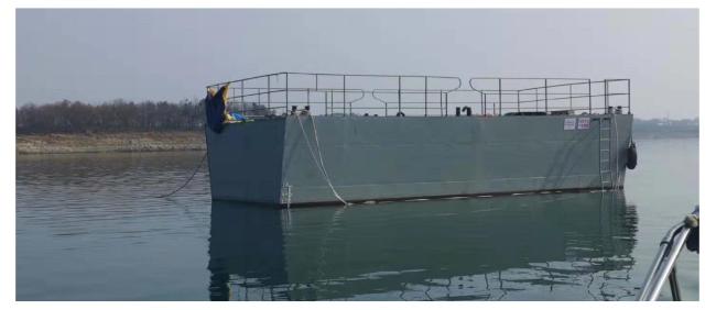
Fig. 10. the experimental model in water. |
Two types of excitation conditions were designed, including shaker conditions and diesel engine conditions. The response acceleration of the base panel was firstly obtained, while the underwater radiated sound power also needed to be measured, with the equipment operating. The vibration measurements were performed by measuring the response acceleration of the base panel, the vibration response of the hull, and the transmitted forces from the equipment to the base. The underwater acoustic measurements were conducted by the cylindrical array to measure the underwater radiated sound power. The principle diagram of the vibration and underwater acoustic testing system is shown in Fig. 11, which includes the arrangement of acceleration sensors and hydrophones, data transmission path, and measured conditions. The acoustic excitation is also included when the engine diesel was installed on the base. The simulated results include mechanical excitation and acoustic excitation. A three-parameter method is used to quantitatively evaluate the well-fitting of experimental and numerical results.
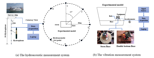
Fig. 11. the principle diagram of the testing system. |
4.1. Validating the first load criterion
For the first load criterion, the generalized forces and the underwater radiated noise need to be verified. During vibration experiments, the acceleration response and the transmitted forces must be measured. Two different load conditions were designed, which the shaker and the diesel engine excited the double bottom base, respectively. The accelerations were measured by acceleration sensors. The transferred forces were measured by force sensors under the shaker condition or by force loops sensors under the diesel engine condition, as shown in Fig. 12. The exciting frequency is 50-200 Hz in the shaker condition and 20-1000 Hz in the diesel engine condition. The validity of the method is verified by comparing the mechanical forces and underwater radiated sound power with the experimental results.
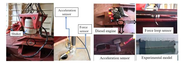
Fig. 12. The experiments for the first load criterion. |
The accelerations are converted to forces by the first load criterion, and the identified forces and the simulated underwater radiated sound power are compared with the experimental results under the shaker condition and the engine diesel condition, as shown in Fig. 13-16. The average force was compared in Fig. 15 under the engine diesel condition.
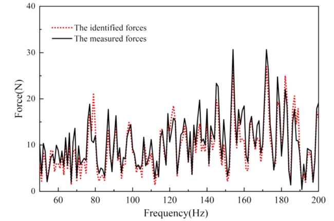
Fig. 13. The identified force by the first load criterion under the shaker. |
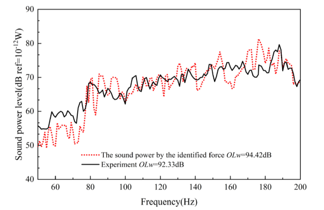
Fig. 14. The sound power by the first load criterion with experiment. |
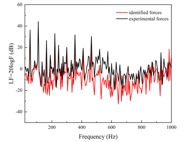
Fig. 15. The identified force by the first load criterion under the diesel engine. |
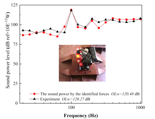
Fig. 16. The power results by the first load criterion under the diesel engine. |
Based on the first load criterion, the calculated results of the two working conditions are summarized in Table 1.
Table 1. The results of the two load conditions based on the first load criterion. |
| Load condition | Comparison object | Overall level error/dB | Correlation coefficient | Standard deviation/dB |
|---|---|---|---|---|
| Shaker | Force | 0.80 | 0.70 | 1.02 |
| Noise | 2.09 | 0.94 | 2.77 | |
| Diesel engine | Force | 1.88 | 0.84 | 6.44 |
| Noise | 0.21 | 0.86 | 3.02 |
The overall level error indicates the calculation accuracy of load identification, while the correlation coefficient and the standard deviation of the error represent the similarity and consistency of the two curves. As can be seen from Table 1, the results show that the consistency of the experimental and simulated force curves matches well, and the peak values and peak frequencies of the sound power curves maintain a good consistency in two load conditions. The trends of the two sound power curves are consistent, and the errors are slight.
4.2. Validating the second load criterion
For the second load criterion, it needs to confirm that the measured underwater radiated noise is between the upper and lower limits determined by the average acceleration load of the base panel. Experimental measurement was performed in two load cases, including the diesel engine rigidly installed on the short base of the double bottom and the round base of the stern. The response acceleration needs to be obtained. Simultaneously the underwater radiated sound power was also measured. The procedure of the experiment is shown below. The diesel engine was installed on the double-bottom short base or the stern round base with the diesel engine operating under the rated power. The acceleration response of the base panel was measured, while the underwater radiated sound power was also measured. The two load conditions are shown in Fig. 17.
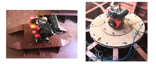
Fig. 17. The two load conditions of the diesel engine. |
The average acceleration loads of the two load conditions are shown in Fig. 18.
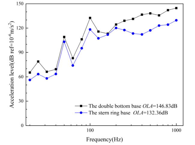
Fig. 18. The measured acceleration loads of the two engine diesel load cases. |
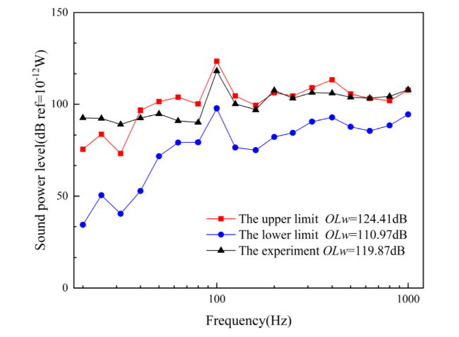
Fig. 19. The upper-lower limits of the sound power with the double-bottom base. |
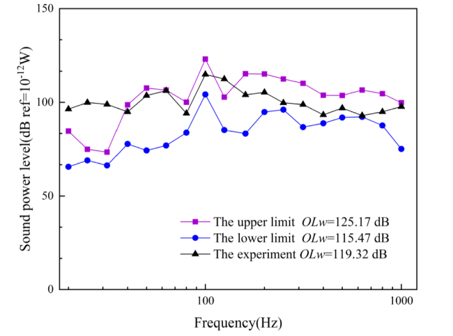
Fig. 20. The upper-lower limits of the sound power with the stern round base. |
The results of the two working conditions are summarized in Table 2.
Table 2. The results of the two load conditions based on the first load criterion. |
| Load condition | Upper limit value/dB | Lower limit value/dB | Energy-averaged value/dB | Experimental results/dB |
|---|---|---|---|---|
| The double-bottom base | 124.41 | 110.97 | 119.36 | 119.87 |
| The stern round base | 127.00 | 115.47 | 120.14 | 119.32 |
It is obvious in Table 2 that the overall level of underwater radiated sound power measured by the experiment is between the upper and lower limits which are determined by the average acceleration based on the second load criterion, and the energy-averaged values are similar to the experimental results with the errors nearby 1 dB. The trends of the sound power curve between the experiment and the simulation are similar, and the peak value and the corresponding frequency band also match well. Therefore, the measured results validate the effectiveness and precision of the second load criterion.
4.3. Validating the third load criterion
For the third load criterion, it takes to validate the acceleration conversion method and the underwater radiated noise predicting method. When predicting mechanical noise through the third load criterion, it must obtain the acceleration loads from the bench testing, the transfer functions of the bench structure, and the transfer functions of the base in a real ship. Meanwhile, the vibroacoustic transfer function of a ship is obtained under the FzMxy load mode. Similar to the previous experiment, the procedure is shown below. Firstly, the diesel engine was mounted on the bench structure and the acceleration load was reported when the diesel engine was running. Secondly, the diesel engine was mounted on the double bottom base, and the acceleration response of the base panel was also measured while the diesel engine was operating at the same power, as shown in Fig. 21. Finally, the underwater radiated noise was measured simultaneously.

Fig. 21. The measurement of acceleration loads on different support foundations. |
The acceleration loads with the diesel engine operating on the different support foundations are obtained as shown in Fig. 22.
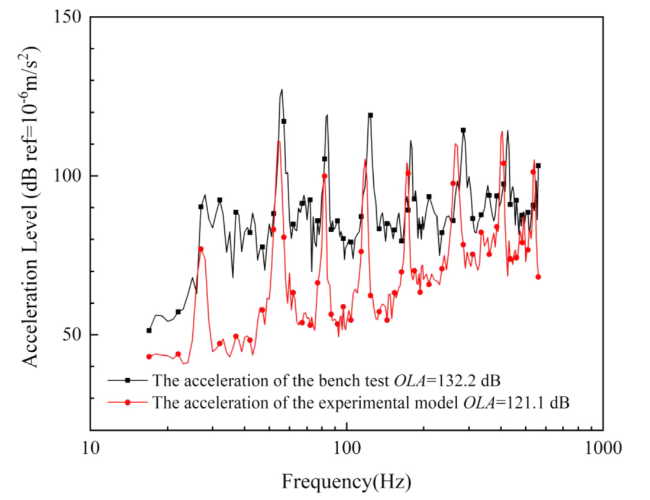
Fig. 22. The acceleration load testing results. |
Based on the load model FzMxy, the transfer function of the bench structure and the double-bottom base are obtained, respectively, shown in Fig. 23. The acceleration load with the diesel engine installed on the base was calculated according to the third load criterion, and compared to the measured results, as shown in Fig. 24. Finally, the vibroacoustic transfer function of the experimental model is also calculated based on the same load model. The radiated sound power generated by the diesel engine is solved according to the third load criterion, and compared with the measured results as shown in Fig. 25.
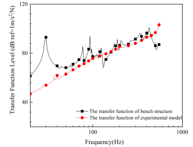
Fig. 23. The transfer function on different support foundations. |
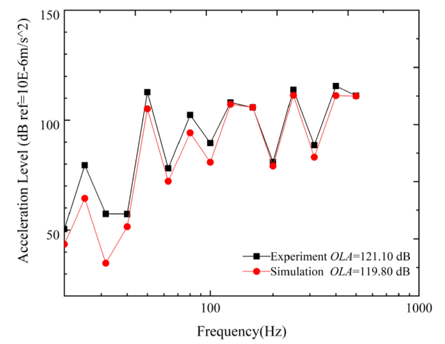
Fig. 24. The comparison of acceleration loads. |
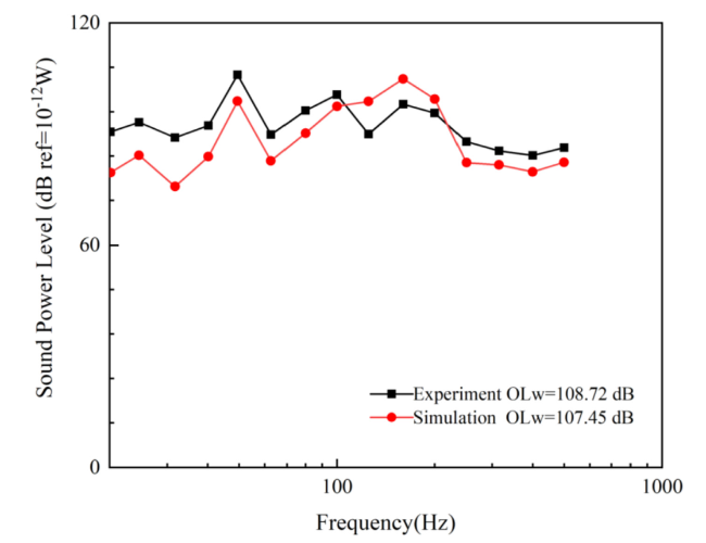
Fig. 25. The comparison of the underwater radiated sound power. |
Based on the third load criterion, the results of the experimental model are summarized in Table 3.
Table 3. The results of the experimental model based on the third load criterion. |
| Comparison Object | The overall level error/dB | Correlation coefficient | Standard deviation/dB |
|---|---|---|---|
| Acceleration | 1.30 | 0.98 | 5.66 |
| Sound power | 1.28 | 0.62 | 8.61 |
As shown in Table 3, the simulated acceleration and sound power obtained by the third load criterion are similar to the experimental results, with the errors being within 3 dB. The trends of the sound power and the acceleration curves match well throughout the frequency band. The results calculated by the third load criterion can characterize the overall level of mechanical noise generated by diesel engines and the distribution of radiated energy in the frequency domain. Therefore, the third load criterion can be also verified by the vibration and hydroacoustic experiment of the model.
5. Conclusion
The loading methods of mechanical equipment to predict mechanical noise in low frequencies are systematically investigated. It defines the generalized force as the standard load to calculate the underwater radiated sound power, as well as the load criterion in which the generalized force is converted from the acceleration. The effect of acceleration load on mechanical noise is first investigated, and three load criteria are proposed based on different types of acceleration loads. These load criteria are finally verified by experimental measurements. The conclusions obtained in this paper are summarized as follows.
1) To predict underwater radiated noise with acceleration loads, it is essential to obtain the acceleration amplitude distribution and phase information. The generalized force can be identified by the first loading criterion.
2) Based on the second load criterion, the upper and lower limits of ships’ underwater radiated sound power can be determined, the energy-averaged value is used to characterize the underwater radiated noise.
3) According to the source descriptor invariance of mechanical equipment and the FzMxy load model, the underwater radiated sound power can be predicted by the third load criterion under, with the acceleration obtained by the bench testing.
4) The significance of the forces and moments can be directly compared by vibroacoustic transfer function based on acceleration, and determine the dominant generalized force components affecting the structural underwater radiated noise in different frequencies.
5) The three-parameter method can quantitatively evaluate the well-fitting of experimental and numerical curves.
Credit author statement
Xi'an Liu: Conceptualization, Writing -Original Draft. Writing -Review & Editing, Data analysis, Validation.
Deqing Yang: Methodology, Supervision, Writing -Review & Editing, Project administration.
Qing Li: Resources, Data Curation, Funding acquisition.
Declaration of Competing Interest
No conflict of interest exists in the submission of this manuscript, and the manuscript is approved by all authors for publication. I would like to declare on behalf of my co-authors that the work described is original research that has not been published previously, and is not under consideration for publication elsewhere. All the authors listed have approved the manuscript that is enclosed.
