
1. Introduction
Internal waves (gravity waves) are only seen on the inside of fluids and are never seen outside. It can be found primarily beneath the ocean's surface layer and atmosphere. The three-dimensional fluid's temperature change is useful in recognising the propagation of gravity waves (internal waves) and the three-dimensional wavelength. When waves, such as winds and other waves, come into touch with internal waves [1], they gain velocity and energy. Wave clouds are primarily interested in atmospheric waves. Internal waves can be seen in Australia's Morning Glory clouds. Many mathematical models and simulations have been developed by the researchers for the interaction and propagation of gravity waves [1], [2], [3], [4], [5].
The mathematical model of shallow fluid assumption can represent internal waves. The ‘shallow fluid’ word asserts that the horizontal scale of the perturbation is more important than the fluid layer's depth [4]. Many models, such as Kelvin waves modelling [6], [7], climate modelling [8], tsunami models [9], [10], and Rossby waves models [7], [11], benefited greatly from the assumption of shallow fluid. Many researchers have used analytical techniques to solve such models [[5], [10], [13], [14], [15]]. Internal waves can be expressed using nonlinear partial differential equations.
The exact solution to such an equation is difficult to calculate. Many numerical and analytical approaches are available as a result; however, numerical methods provide the discrete points of the solution. Analytical procedures began to gain popularity. There are various analytical methods for determining the answer to issues [16], [17], [18], [19]. HAM and VIM [20] and EADM [5] were used to solve partial differential equations of internal atmospheric waves.
Liao invented the Homotopy Analysis Method [21], [22], [23] in 1992, which proved to be very effective in locating the approximate convergent solution to nonlinear problems. This method has been used by many researchers to solve arising nonlinear problems [24], [25], [26], [27], [28], [29], [30], [31], [32]. El-Tawil and Husein improved HAM and introduced the q-HAM [33], [34] approach for faster convergence. Later, numerous researchers integrated transforms such as Laplace transform [35], Sumudu transform [36], Aboodh transforms [37], and Elzaki transform [38] with q-HAM to discover a superior fractional order differential equation solution. Sartanpara and Meher proposed the q-HAShTM [12] in 2021, combining the Shehu Transform [39], [40] and the q-HAM for solving time-fractional Zakharov-Kuznetsov equations.
In 1965 [41], the fuzzy set was introduced, and later on, uncertainty was used in every branch of mathematics and science. Puri and Ralescu [42] explained the differentiation of fuzzy functions. Researchers later used fuzzy functions and parameters to tackle problems in various domains [15], [43], [44]. Chakraverty and Perera provided a brief overview of recent computational and fuzzy mathematics [45] and Karunakar and Chakravarty [46] used fuzzy approach and solved shallow water wave equations.
The fuzzy theory helps explain the nature of challenges in any real-world topic that is uncertain. To overcome this uncertainty, we consider a time-fractional fuzzy atmospheric internal wave model considering fuzzy parameters.
This paper applies the q-HAShTM to the time-fractional atmospheric internal wave mathematical model and fuzzy-fractional atmospheric internal wave model with fuzzy initial conditions.
2. Preliminaries
2.1. Shehu transform
Let $g\left( t \right)\in A$ where
$A=\left\{ g\left( t \right)|\exists K,{{\kappa }_{1}},{{\kappa }_{2}}>0,\left| g\left( t \right) \right|Kexp\left( \frac{\left| t \right|}{{{\kappa }_{i}}} \right),\text{if}t\in {{\left(-1 \right)}^{i}}\times \left[ 0,\infty \right) \right\},$
then Shehu Transform [39] of $g\left( t \right)$
$G\left( s,u \right)=\mathcal{S}\left[ g\left( t \right) \right]=\underset{0}{\overset{\infty }{\mathop \int }}\,\exp \left( \frac{-st}{u} \right)g\left( t \right)dt.$
where, $s>0$ and $u>0$.
Few results using Eq. (2.1)
1. For any constant $a$, $\mathcal{S}\left[ a \right]=a\left( \frac{u}{s} \right)$.
2. $\frac{\mathcal{S}\left[ {{t}^{a}} \right]}{ \Gamma \left( a+1 \right)}=\frac{{{u}^{a+1}}}{{{s}^{a+1}}},a>-1$.
3. $\mathcal{S}\left[ a{{g}_{1}}\left( t \right)\pm b{{g}_{2}}\left( t \right) \right]=a\mathcal{S}\left[ {{g}_{1}}\left( t \right) \right]\pm b\mathcal{S}\left[ {{g}_{2}}\left( t \right) \right]$
2.2. Inverse Shehu transform
Inverse Shehu transform [39] of $G\left( s,u \right)=\mathcal{S}\left[ g\left( t \right) \right]$ is given by
${{\mathcal{S}}^{-1}}\left[ G\left( s,u \right) \right]=g\left( t \right)=\underset{\delta \to \infty }{\mathop{\lim }}\,\frac{1}{2\pi i}\underset{\gamma +i\delta }{\overset{\gamma-i\delta }{\mathop \int }}\,\frac{1}{u}\exp \left( \frac{st}{u} \right)G\left( s,u \right)ds.$
2.3. Caputo fractional derivative's Shehu transform
$\mathcal{S}\left[ D_{t}^{\alpha }g\left( t \right) \right]=\left( \frac{{{s}^{\alpha }}}{{{u}^{\alpha }}} \right)G\left( s,u \right)-\underset{k=0}{\overset{n-1}{\mathop \sum }}\,\left( \frac{{{s}^{\alpha-k-1}}}{{{u}^{\alpha-k-1}}} \right){{g}^{\left( k \right)}}\left( {{0}^{+}} \right).$
where, $\alpha \in \left( n-1,n \right]$ is positive number and $n$ is natural number.
2.4. Fuzzy set
$\tilde{P}=\left\{ \left( p,m\left( p \right) \right):p\in U,m\left( p \right)\in \left[ 0,1 \right] \right\}.$
2.5. Fuzzy number
2.6. Triangular fuzzy number
$m\left( p \right)=\left\{ \begin{matrix} 0, & p\le {{P}_{l}} \\ \frac{p-{{P}_{l}}}{{{P}_{c}}-{{P}_{l}}} & {{P}_{l}}\le p\le {{P}_{c}} \\ \frac{{{P}_{u}}-p}{{{P}_{u}}-{{P}_{c}}} & {{P}_{c}}\le p\le {{P}_{u}} \\ 0, & p>{{P}_{u}}. \\ \end{matrix} \right.$
Here, ${{P}_{l}}$, ${{P}_{c}}$ and ${{P}_{u}}$ represent the lower fuzzy value, center fuzzy value and upper fuzzy value, respectively.
2.7. r-cut
$\widetilde{P}=\left[ {{P}_{l}},{{P}_{c}},{{P}_{u}} \right]=\left[ \left( {{P}_{c}}-{{P}_{l}} \right)r+{{P}_{l}},{{P}_{u}}-\left( {{P}_{u}}-{{P}_{c}} \right)r \right],\text{Where}r\in \left[ 0,1 \right]$
2.8. Parametric formulation
We can write an interval $J=\left[ \underline{J},\bar{J} \right]$ in the parametric form as following [45] :
$J=\beta \left( \bar{J}-\underline{J} \right)+\underline{J},\beta \in \left[ 0,1 \right]$
3. q-Homotopy analysis Shehu transform method [12]
To understand the basic idea of the q-HAShTM, we consider the following system of nonlinear partial differential equations with fractional order $\alpha \in \left( n-1,n \right]$
$\begin{align} & D_{t}^{\alpha }{{\mu }_{1}}\left( x,t \right)+{{\mathcal{L}}_{1}}\left( {{\mu }_{1}}\left( x,t \right) \right),{{\mu }_{2}}\left( x,t \right),\cdots,\left. {{\mu }_{i}}\left( x,t \right) \right) \\ & +{{N}_{1}}\left( {{\mu }_{1}}\left( x,t \right) \right),{{\mu }_{2}}\left( x,t \right),\cdots,\left. {{\mu }_{i}}\left( x,t \right) \right)={{R}_{1}}\left( x,t \right), \\ & D_{t}^{\alpha }{{\mu }_{2}}\left( x,t \right)+{{\mathcal{L}}_{2}}\left( {{\mu }_{1}}\left( x,t \right) \right),{{\mu }_{2}}\left( x,t \right),\cdots,\left. {{\mu }_{i}}\left( x,t \right) \right) \\ & +{{N}_{2}}\left( {{\mu }_{1}}\left( x,t \right) \right),{{\mu }_{2}}\left( x,t \right),\cdots,\left. {{\mu }_{i}}\left( x,t \right) \right)={{R}_{2}}\left( x,t \right), \\ & \vdots \\ & D_{t}^{\alpha }{{\mu }_{i}}\left( x,t \right)+{{\mathcal{L}}_{i}}\left( {{\mu }_{1}}\left( x,t \right) \right),{{\mu }_{2}}\left( x,t \right),\cdots,\left. {{\mu }_{i}}\left( x,t \right) \right) \\ & +{{N}_{1}}\left( {{\mu }_{1}}\left( x,t \right) \right),{{\mu }_{2}}\left( x,t \right),\cdots,\left. {{\mu }_{i}}\left( x,t \right) \right)={{R}_{i}}\left( x,t \right), \\ \end{align}$
where $i\in \mathbb{N}$, $D_{t}^{\alpha }{{\mu }_{i}}\left( x,t \right)$ stand for the Caputo fractional derivatives of functions, ${{N}_{i}}$ are nonlinear differential operators, ${{\mathcal{L}}_{i}}\left( {{\mu }_{i}}\left( x,t \right) \right)$ are linear differential operators and source terms are represented by ${{R}_{i}}\left( x,t \right)$.
Taking the Shehu Transform on Eq. (3.1), we obtain
$\begin{align} & {{\left( \frac{s}{u} \right)}^{\alpha }}\mathcal{S}\left[ {{\mu }_{1}}(x,t) \right]-\sum\nolimits_{k=0}^{n-1}{{{\left( \frac{s}{u} \right)}^{\alpha-k-1}}\mu _{1}^{(k)}(x,0)} \\ & +\mathcal{S}\left[ {{\mathcal{L}}_{1}}\left( {{\mu }_{1}}\left( x,t \right),{{\mu }_{2}}\left( x,t \right),\ldots,{{\mu }_{i}}\left( x,t \right) \right) \right] \\ & +\mathcal{S}\left[ {{N}_{1}}\left( {{\mu }_{1}}\left( x,t \right),{{\mu }_{2}}\left( x,t \right),\ldots,{{\mu }_{i}}\left( x,t \right) \right) \right]=\mathcal{S}\left[ {{R}_{1}}\left( x,t \right) \right], \\ & {{\left( \frac{s}{u} \right)}^{\alpha }}\mathcal{S}\left[ {{\mu }_{2}}(x,t) \right]-\sum\nolimits_{k=0}^{n-1}{{{\left( \frac{s}{u} \right)}^{\alpha-k-1}}\mu _{2}^{(k)}(x,0)} \\ & +\mathcal{S}\left[ {{\mathcal{L}}_{2}}\left( {{\mu }_{1}}\left( x,t \right),{{\mu }_{2}}\left( x,t \right),\ldots,{{\mu }_{i}}\left( x,t \right) \right) \right] \\ & +\mathcal{S}\left[ {{N}_{2}}\left( {{\mu }_{1}}\left( x,t \right),{{\mu }_{2}}\left( x,t \right),\ldots,{{\mu }_{i}}\left( x,t \right) \right) \right]=\mathcal{S}\left[ {{R}_{2}}\left( x,t \right) \right], \\ & \vdots \\ & {{\left( \frac{s}{u} \right)}^{\alpha }}\mathcal{S}\left[ {{\mu }_{i}}(x,t) \right]-\sum\nolimits_{k=0}^{n-1}{{{\left( \frac{s}{u} \right)}^{\alpha-k-1}}\mu _{i}^{(k)}(x,0)} \\ & +\mathcal{S}\left[ {{\mathcal{L}}_{i}}\left( {{\mu }_{1}}\left( x,t \right),{{\mu }_{2}}\left( x,t \right),\ldots,{{\mu }_{i}}\left( x,t \right) \right) \right] \\ & +\mathcal{S}\left[ {{N}_{i}}\left( {{\mu }_{1}}\left( x,t \right),{{\mu }_{2}}\left( x,t \right),\ldots,{{\mu }_{i}}\left( x,t \right) \right) \right]=\mathcal{S}\left[ {{R}_{i}}\left( x,t \right) \right]. \\ \end{align}$
We can simplify Eq. (3.2) as following
$\begin{align} & \mathcal{S}\left[ {{\mu }_{1}}(x,t) \right]-{{\left( \frac{u}{s} \right)}^{\alpha }}\sum\nolimits_{k=0}^{n-1}{{{\left( \frac{s}{u} \right)}^{\alpha-k-1}}\mu _{1}^{(k)}(x,0)} \\ & +{{\left( \frac{u}{s} \right)}^{\alpha }}\mathcal{S}\left[ {{\mathcal{L}}_{1}}\left( {{\mu }_{1}}\left( x,t \right),{{\mu }_{2}}\left( x,t \right),\ldots,{{\mu }_{i}}\left( x,t \right) \right) \right. \\ & +\left. {{N}_{1}}\left( {{\mu }_{1}}\left( x,t \right),{{\mu }_{2}}\left( x,t \right),\ldots,{{\mu }_{i}}\left( x,t \right) \right)-{{R}_{1}}\left( x,t \right) \right]=0, \\ & \mathcal{S}\left[ {{\mu }_{2}}(x,t) \right]-{{\left( \frac{u}{s} \right)}^{\alpha }}\sum\nolimits_{k=0}^{n-1}{{{\left( \frac{s}{u} \right)}^{\alpha-k-1}}\mu _{2}^{(k)}(x,0)} \\ & +{{\left( \frac{u}{s} \right)}^{\alpha }}\mathcal{S}\left[ {{\mathcal{L}}_{2}}\left( {{\mu }_{1}}\left( x,t \right),{{\mu }_{2}}\left( x,t \right),\ldots,{{\mu }_{i}}\left( x,t \right) \right) \right. \\ & +\left. {{N}_{2}}\left( {{\mu }_{1}}\left( x,t \right),{{\mu }_{2}}\left( x,t \right),\ldots,{{\mu }_{i}}\left( x,t \right) \right)-{{R}_{2}}\left( x,t \right) \right]=0, \\ & \vdots \\ & \mathcal{S}\left[ {{\mu }_{i}}(x,t) \right]-{{\left( \frac{u}{s} \right)}^{\alpha }}\sum\nolimits_{k=0}^{n-1}{{{\left( \frac{s}{u} \right)}^{\alpha-k-1}}\mu _{i}^{(k)}(x,0)} \\ & +{{\left( \frac{u}{s} \right)}^{\alpha }}\mathcal{S}\left[ {{\mathcal{L}}_{i}}\left( {{\mu }_{1}}\left( x,t \right),{{\mu }_{2}}\left( x,t \right),\ldots,{{\mu }_{i}}\left( x,t \right) \right) \right. \\ & +\left. {{N}_{i}}\left( {{\mu }_{1}}\left( x,t \right),{{\mu }_{2}}\left( x,t \right),\ldots,{{\mu }_{i}}\left( x,t \right) \right)-{{R}_{i}}\left( x,t \right) \right]=0. \\ \end{align}$
Nonlinear operators can be defined as
$\begin{array}{l} \mathcal{N}_{1} {\left[\omega_{1}(x, t ; q), \omega_{2}(x, t ; q), \ldots, \omega_{i}(x, t ; q)\right]=} \\ \mathcal{S}\left[\omega_{1}(x, t ; q)\right]-\left(\frac{u}{s}\right)^{\alpha} \sum_{k=0}^{n-1}\left(\frac{s}{u}\right)^{\alpha-k-1} \omega_{1}^{(k)}\left(x, 0^{+} ; q\right) \\ +\left(\frac{u}{s}\right)^{\alpha} \mathcal{S}\left[\mathcal{L}_{1}\left(\omega_{1}(x, t ; q), \omega_{2}(x, t ; q), \ldots, \omega_{i}(x, t ; q)\right)\right. \\ \left.+N_{1}\left(\omega_{1}(x, t ; q), \omega_{2}(x, t ; q), \ldots, \omega_{i}(x, t ; q)\right)-R_{1}(x, t)\right] \\ \mathcal{N}_{2} {\left[\omega_{1}(x, t ; q), \omega_{2}(x, t ; q), \ldots \omega_{i}(x, t ; q)\right]=} \\ \mathcal{S}\left[\omega_{2}(x, t ; q)\right]-\left(\frac{u}{s}\right)^{\alpha} \sum_{k=0}^{n-1}\left(\frac{s}{u}\right)^{\alpha-k-1} \omega_{2}^{(k)}\left(x, 0^{+} ; q\right) \\ +\left(\frac{u}{s}\right)^{\alpha} \mathcal{S}\left[\mathcal{L}_{2}\left(\omega_{1}(x, t ; q), \omega_{2}(x, t ; q), \ldots, \omega_{i}(x, t ; q)\right)\right. \\ \left.+N_{2}\left(\omega_{1}(x, t ; q), \omega_{2}(x, t ; q), \ldots, \omega_{i}(x, t ; q)\right)-R_{2}(x, t)\right] \\ \vdots \\ \mathcal{N}_{i} {\left[\omega_{1}(x, t ; q), \omega_{2}(x, t ; q), \ldots, \omega_{i}(x, t ; q)\right]=} \\ \mathcal{S}\left[\omega_{i}(x, t ; q)\right]-\left(\frac{u}{s}\right)^{\alpha} \sum_{k=0}^{n-1}\left(\frac{s}{u}\right)^{\alpha-k-1} \omega_{i}^{(k)}\left(x, 0^{+} ; q\right) \\ +\left(\frac{u}{s}\right)^{\alpha} \mathcal{S}\left[\mathcal{L}_{i}\left(\omega_{1}(x, t ; q), \omega_{2}(x, t ; q), \ldots, \omega_{i}(x, t ; q)\right)\right. \\ \left.+N_{i}\left(\omega_{1}(x, t ; q), \omega_{2}(x, t ; q), \ldots, \omega_{i}(x, t ; q)\right)-R_{i}(x, t)\right] \end{array}$
where ${{\omega }_{i}}\left( x,t,q \right)$ are real-valued functions of x, t and $q\in \left[ 0,\frac{1}{n} \right]\left( n\ge 1 \right)$, q is an embedding parameter.
Now, we build homotopy as
$\begin{matrix} (1-n q) \mathcal{S}\left[\omega_{1}(x, t ; q)-\mu_{10}(x, t)\right]=\hbar q H_{1}(x, t) \mathscr{N}_{1}\left[\omega_{1}(x, t ; q), \omega_{2}(x, t ; q), \ldots, \omega_{i}(x, t ; q)\right] \\ (1-n q) \mathcal{S}\left[\omega_{2}(x, t ; q)-\mu_{20}(x, t)\right]=\hbar q H_{2}(x, t) \mathscr{N}_{2}\left[\omega_{1}(x, t ; q), \omega_{2}(x, t ; q), \ldots, \omega_{i}(x, t ; q)\right] \\ \vdots \\ (1-n q) \mathcal{S}\left[\omega_{i}(x, t ; q)-\mu_{i 0}(x, t)\right]=\hbar q H_{i}(x, t) \mathscr{N}_{i}\left[\omega_{1}(x, t ; q), \omega_{2}(x, t ; q), \ldots, \omega_{i}(x, t ; q)\right] \\ \end{matrix}$
which are known as Zero-order deformation equations, where $\mathcal{S}$ stands for Shehu transform, $\hbar \left( \ne 0 \right)$ is auxiliary parameter, ${{H}_{i}}\left( x,t \right)\left( \ne 0 \right)$ are auxiliary functions, our initial guesses of ${{\mu }_{i}}\left( x,t \right)$ are ${{\mu }_{i}}_{0}\left( x,t \right)$ and ${{\omega }_{i}}\left( x,t;q \right)$ are unknown functions. For q=0, ${{\omega }_{i}}\left( x,t;0 \right)$ and for $q=\frac{1}{n}$, ${{\omega }_{i}}\left( x,t;\frac{1}{n} \right)$ hold following results
$\begin{matrix} \omega_{1}(x, t ; 0)=\mu_{10}(x, t), \quad \omega_{1}\left(x, t ; \frac{1}{n}\right)=\mu_{1}(x, t) \\ \omega_{2}(x, t ; 0)=\mu_{20}(x, t), \quad \omega_{2}\left(x, t ; \frac{1}{n}\right)=\mu_{2}(x, t), \\ \vdots \\ \omega_{i}(x, t ; 0)=\mu_{i 0}(x, t), \quad \omega_{i}\left(x, t ; \frac{1}{n}\right)=\mu_{i}(x, t) \\ \end{matrix}$
So, as the value of q increases from 0 to $\frac{1}{n}$, the solutions ${{\omega }_{i}}\left( x,t;q \right)$ converge from our initial assumption ${{\mu }_{i}}_{0}\left( x,t \right)$ to the solutions ${{\mu }_{i}}\left( x,t \right)$. Expansions of ${{\omega }_{i}}\left( x,t;q \right)$ in the Taylor series with respect to q
$\begin{array}{c} \omega_{1}(x, t ; q)=\mu_{10}(x, t)+\sum_{m=1}^{\infty} \mu_{1_{m}}(x, t) q^{m} \\ \omega_{2}(x, t ; q)=\mu_{20}(x, t)+\sum_{m=1}^{\infty} \mu_{2_{m}}(x, t) q^{m} \\ \vdots \\ \omega_{i}(x, t ; q)=\mu_{i 0}(x, t)+\sum_{m=1}^{\infty} \mu_{i m}(x, t) q^{m} \end{array}$
where ${{\mu }_{i}}_{m}\left( x,t \right)$ stand for
$\begin{array}{c} \mu_{i m}(x, t)=\left.\frac{1}{m!} \frac{\partial^{m} \omega_{i}(x, t ; q)}{\partial q^{m}}\right|_{q=0} \\ \mu_{i m}(x, t)=\left.\frac{1}{m!} \frac{\partial^{m} \omega_{i}(x, t ; q)}{\partial q^{m}}\right|_{q=0} \\ \vdots \\ \mu_{i m}(x, t)=\left.\frac{1}{m!} \frac{\partial^{m} \omega_{i}(x, t ; q)}{\partial q^{m}}\right|_{q=0} \end{array}$
At $q=\frac{1}{n}$, the choice of ${{\mu }_{i}}_{0}\left( x,t \right)$, n, $\hbar$ is proper than Eq. (3.7) converge to the one of the solutions of Eq. (3.1)
$\begin{array}{c} \mu_{1}(x, t)=\mu_{10}(x, t)+\sum_{m=1}^{\infty} \mu_{1_{m}}(x, t)\left(\frac{1}{n}\right)^{m} \\ \mu_{2}(x, t)=\mu_{20}(x, t)+\sum_{m=1}^{\infty} \mu_{2 m}(x, t)\left(\frac{1}{n}\right)^{m} \\ \vdots \\ \mu_{i}(x, t)=\mu_{i 0}(x, t)+\sum_{m=1}^{\infty} \mu_{i m}(x, t)\left(\frac{1}{n}\right)^{m} \end{array}$
We define vectors ${{\overrightarrow{{{\mu }_{i}}}}_{m}}$ as following
$\begin{array}{c} \overrightarrow{\mu}_{{1 m}}=\left\{\mu_{10}(x, t), \mu_{11}(x, t), \mu_{12}(x, t), \ldots, \mu_{1 m}(x, t)\right\}, \\ \overrightarrow{\mu}_{{2 m}}=\left\{\mu_{20}(x, t), \mu_{21}(x, t), \mu_{22}(x, t), \ldots, \mu_{2 m}(x, t)\right\}, \\ \vdots \\ \overrightarrow{\mu}_{{i m}}=\left\{\mu_{i 0}(x, t), \mu_{i 1}(x, t), \mu_{i 2}(x, t), \ldots, \mu_{i m}(x, t)\right\}. \end{array}$
Now, Eq. (3.5) are divided by m! and m-times differentiate with respect to q and substituting q=0, we obtain deformation equations of mth-order as follow
$\begin{matrix} \mathcal{S}\left[\mu_{1 m}(x, t)-\psi_{m} \mu_{1_{m-1}}(x, t)\right]=\hbar H_{1}(x, t) \mathscr{R}_{1 m}\left(\overrightarrow{\mu}_{{1 m-1}}, \overrightarrow{\mu}_{{2 m-1}}, \ldots, \overrightarrow{\mu}_{{i m-1}}\right), \\ \mathcal{S}\left[\mu_{2 m}(x, t)-\psi_{m} \mu_{2 m-1}(x, t)\right]=\hbar H_{2}(x, t) \mathscr{R}_{2 m}\left(\vec{\mu}_{1 m-1}, \overrightarrow{\mu}_{{2 m-1}}, \ldots, \overrightarrow{\mu}_{{i m-1}}\right) \text {, } \\ \vdots \\ \mathcal{S}\left[\mu_{i m}(x, t)-\psi_{m} \mu_{i m-1}(x, t)\right]=\hbar H_{i}(x, t) \mathscr{R}_{i m}\left(\overrightarrow{\mu}_{{1 m-1}}, \overrightarrow{\mu}_{{2 m-1}}, \ldots, \overrightarrow{\mu}_{{i m-1}}\right), \\ \end{matrix}$
where ${{\mathscr{R}}_{i}}_{m}\left( {{\overrightarrow{{{\mu }_{1}}}}_{m-1}},{{\overrightarrow{{{\mu }_{2}}}}_{m-1}},\ldots,{{\overrightarrow{{{\mu }_{i}}}}_{m-1}} \right)$ stand for
$\begin{matrix} \begin{array}{l} \quad \mathcal{R}_{1 m}\left(\vec{\mu}_{1 m-1}, \vec{\mu}_{2 m-1}, \ldots, \vec{\mu}_{i m-1}\right)= \\ \left.\quad \frac{1}{(m-1)!} \frac{\partial^{m-1} \mathcal{N}_{1}\left[\omega_{1}(x, t ; q), \omega_{2}(x, t ; q), \ldots, \omega_{i}(x, t ; q)\right]}{\partial q^{m-1}}\right|_{q=0} \\ =\mathcal{S}\left[\mu_{1 m-1}(x, t)\right]-\left(1-\frac{\psi_{m}}{n}\right)\left[\left(\frac{u}{s}\right)^{\alpha} \sum_{k=0}^{n-1}\left(\frac{s}{u}\right)^{\alpha-k-1} \mu_{1}(k)(x, 0)\right] \\ \quad+\left(\frac{u}{s}\right)^{\alpha} \mathcal{S}\left[\mathcal{L}_{1}\left(\mu_{1 m-1}(x, t), \mu_{2 m-1}(x, t), \ldots, \mu_{i m-1}(x, t)\right)\right. \\ \left.\quad+\left.\frac{1}{(m-1)!} \frac{\partial^{m-1} N_{1}\left(\omega_{1}(x, t ; q), \omega_{2}(x, t ; q), \ldots, \omega_{i}(x, t ; q)\right)}{\partial q^{m-1}}\right|_{q=0}+\left(1-\frac{\psi_{m}}{n}\right) R_{1}(x, t)\right] \end{array} \\ \begin{array}{l} \mathcal{R}_{2 m}\left(\vec{\mu}_{1 m-1}, \vec{\mu}_{2 m-1}, \ldots, \vec{\mu}_{i m-1}\right)= \\ \left.\quad \frac{1}{(m-1)!} \frac{\partial^{m-1} \mathcal{N}_{2}\left[\omega_{1}(x, t ; q), \omega_{2}(x, t ; q), \ldots, \omega_{i}(x, t ; q)\right]}{\partial q^{m-1}}\right|_{q=0} \\ =\mathcal{S}\left[\mu_{2 m-1}(x, t)\right]-\left(1-\frac{\psi_{m}}{n}\right)\left[\left(\frac{u}{s}\right)^{\alpha} \sum_{k=0}^{n-1}\left(\frac{s}{u}\right)^{\alpha-k-1} \mu_{2}(k)(x, 0)\right] \\ \quad+\left(\frac{u}{s}\right)^{\alpha} \mathcal{S}\left[\mathcal{L}_{2}\left(\mu_{1 m-1}(x, t), \mu_{2 m-1}(x, t), \ldots, \mu_{i m-1}(x, t)\right)\right. \\ \left.\quad+\left.\frac{1}{(m-1)!} \frac{\partial^{m-1} N_{2}\left(\omega_{1}(x, t ; q), \omega_{2}(x, t ; q), \ldots, \omega_{i}(x, t ; q)\right)}{\partial q^{m-1}}\right|_{q=0}+\left(1-\frac{\psi_{m}}{n}\right) R_{2}(x, t)\right] \end{array} \\ \vdots \\ \begin{array}{l} \quad \mathcal{R}_{i m}\left(\vec{\mu}_{1 m-1}, \vec{\mu}_{2 m-1}, \ldots, \vec{\mu}_{i m-1}\right)= \\ \left.\quad \frac{1}{(m-1)!} \frac{\partial^{m-1} \mathcal{N}_{2}\left[\omega_{1}(x, t ; q), \omega_{2}(x, t ; q), \ldots, \omega_{i}(x, t ; q)\right]}{\partial q^{m-1}}\right|_{q=0} \\ =\mathcal{S}\left[\mu_{i m-1}(x, t)\right]-\left(1-\frac{\psi_{m}}{n}\right)\left[\left(\frac{u}{s}\right)^{\alpha} \sum_{k=0}^{n-1}\left(\frac{s}{u}\right)^{\alpha-k-1} \mu_{i}^{(k)}(x, 0)\right] \\ \quad+\left(\frac{u}{s}\right)^{\alpha} \mathcal{S}\left[\mathcal{L}_{2}\left(\mu_{1 m-1}(x, t), \mu_{2 m-1}(x, t), \ldots, \mu_{i m-1}(x, t)\right)\right. \\ \left.\quad+\left.\frac{1}{(m-1)!} \frac{\partial^{m-1} N_{i}\left(\omega_{1}(x, t ; q), \omega_{2}(x, t ; q), \ldots, \omega_{i}(x, t ; q)\right)}{\partial q^{m-1}}\right|_{q=0}+\left(1-\frac{\psi_{m}}{n}\right) R_{2}(x, t)\right] \end{array} \\ \end{matrix} $
and
${{\psi }_{m}}=\left\{ \begin{matrix} 0, & m\le 1 \\ n, & m>1. \\ \end{matrix} \right.$
Applying the inverse Shehu Transform on Eq. (3.11),
$\begin{array}{c} \mu_{1 m}(x, t)=\psi_{m} \mu_{1 m-1}(x, t)+\mathcal{S}^{-1}\left[\hbar H_{1}(x, t) \mathscr{R}_{1 m}\left(\vec{\mu}_{1 m-1}, \overrightarrow{\mu}_{{2 m-1}}, \ldots, \overrightarrow{\mu}_{{i m-1}}\right)\right] \\ \mu_{2 m}(x, t)=\psi_{m} \mu_{2 m-1}(x, t)+\mathcal{S}^{-1}\left[\hbar H_{2}(x, t) \mathscr{R}_{2 m}\left(\vec{\mu}_{1 m-1}, \overrightarrow{\mu}_{{2 m-1}}, \ldots, \overrightarrow{\mu}_{{i m-1}}\right)\right] \\ \vdots \\ \mu_{i m}(x, t)=\psi_{m} \mu_{i m-1}(x, t)+\mathcal{S}^{-1}\left[\hbar H_{i}(x, t) \mathscr{R}_{i m}\left(\vec{\mu}_{1 m-1}, \overrightarrow{\mu}_{{2 m-1}}, \ldots, \overrightarrow{\mu}_{{i m-1}}\right)\right] \end{array}$
After solving the Eq. (3.14), we get ${{\mu }_{i}}_{m}\left( x,t \right)$ (for m=1,2,…), and the approximate series solutions can be written as
$\begin{array}{c} \mu_{1}(x, t)=\sum_{m=0}^{\infty} \mu_{1 m}(x, t)\left(\frac{1}{n}\right)^{m} \\ \mu_{2}(x, t)=\sum_{m=0}^{\infty} \mu_{2 m}(x, t)\left(\frac{1}{n}\right)^{m} \\ \vdots \\ \mu_{i}(x, t)=\sum_{m=0}^{\infty} \mu_{i m}(x, t)\left(\frac{1}{n}\right)^{m} \end{array}$
Eq. (3.15), the series solutions will surely be convergent in the presence of $\hbar$ which controls the converges of the series solution.
4. Formulation of atmospheric internal waves model with fractional and fuzzy approach
Nonlinear partial differential equations can be used to describe internal waves in the atmosphere. The primary equation of the shallow fluid assumption was used to build the model. The fundamental equations of fluid motion in the differential form are derived from the conservation of mass and momentum. The wavelength of shallow fluid is greater than the depth of the fluid layer, as the name implies. The assumption is that the atmosphere is hydrostatic and autobarotropic, with a constant density in space (homogeneous fluid). The system can be presented as [5,20],
$\begin{array}{l} (v(x, t))_{t}+v(x, t)(v(x, t))_{x}-f v(x, t)+g(\eta(x, t))_{x}=0 \\ (v(x, t))_{t}+v(x, t)(v(x, t))_{x}-f v(x, t)+g H=0 \\ (\eta(x, t))_{t}+v(x, t)(\eta(x, t))_{x}-H v(x, t)+\eta(x, t)(v(x, t))_{x}=0 \end{array}$
where x represents the coordinate of space, t stands for time. υ and ν are the are cartesian velocity which are depending on x and t. η is fluid's depth, f=2Ω sinθ, where $\theta =\frac{\pi }{3}$ and Ω=7.29×10⁻⁵ rads−1, constant gravitational acceleration g=9.8 ms−2 and the constant of pressure gradient of desired magnitude $H=-\frac{f}{g}\bar{U}$, where $\bar{U}$=2.5ms−1 is mean geostrophic speed. The initial conditions of Eq. (4.1) are
$\begin{array}{l} v(x, 0)=e^{x} \operatorname{sech}^{2}(x) \\ v(x, 0)=2 x \operatorname{sech}^{2}(2 x) \\ \eta(x, 0)=x^{2} \operatorname{sech}^{2}(2 x) \end{array}$
Here, we can construct the time-fraction model for the atmospheric internal waves as following :
$\begin{array}{l} D_{t}^{\alpha} v(x, t)+v(x, t)(v(x, t))_{x}-f v(x, t)+g(\eta(x, t))_{x}=0 \\ D_{t}^{\alpha} v(x, t)+v(x, t)(v(x, t))_{x}-f v(x, t)+g H=0 \\ D_{t}^{\alpha} \eta(x, t)+v(x, t)(\eta(x, t))_{x}-H v(x, t)+\eta(x, t)(v(x, t))_{x}=0. \end{array}$
where $\alpha \in \left[ 0,1 \right]$ and the same initial conditions (4.2) can be applicable. As there are always uncertainty in real world phenomena. For fuzzy-fractional model, we can take fuzzy number for the coefficient of the initial condition as
$\begin{array}{l} \tilde{v}(x, 0 ; r, \beta)=\tilde{A} e^{x} \operatorname{sech}^{2}(x) \\ \tilde{v}(x, 0 ; r, \beta)=\tilde{B} x \operatorname{sech}^{2}(2 x) \\ \tilde{\eta}(x, 0 ; r, \beta)=\tilde{C} x^{2} \operatorname{sech}^{2}(2 x) \end{array} $
where $\tilde{A}$, $\tilde{B}$ and $\tilde{C}$ are triangular fuzzy numbers as following :
$\begin{array}{l} \tilde{A}=[0,1,2], \\ \tilde{B}=[1,2,3] \\ \tilde{C}=[0,1,2] \end{array}$
Applying r-cut on triangular fuzzy number, we get
$\begin{aligned} \widetilde{A} & =[r, 2-r] \\ \widetilde{B} & =[r+1,3-r] \\ \widetilde{C} & =[r, 2-r] \end{aligned}$
Converting it to another parameter, we obtain
$\begin{array}{l} \tilde{A}=(2 \beta(1-r)+r), \\ \tilde{B}=(2 \beta(1-r)+r+1) \\ \tilde{C}=(2 \beta(1-r)+r) \end{array}$
So the fuzzy-time-fractional atmospheric internal wave model can be written as
$\begin{array}{c} D_{t}^{\alpha} \tilde{v}(x, t ; r, \beta)+\tilde{v}(\tilde{v}(x, t ; r, \beta))_{x}-f \tilde{v}(x, t ; r, \beta)+g(\tilde{\eta}(x, t ; r, \beta))_{x}=0 \\ D_{t}^{\alpha} \tilde{v}(x, t ; r, \beta)+\tilde{v}(x, t ; r, \beta)(\tilde{v}(x, t ; r, \beta))_{x}-f \tilde{v}(x, t ; r, \beta)+g H=0 \\ D_{t}^{\alpha} \tilde{\eta}(x, t ; r, \beta)+\tilde{v}(x, t ; r, \beta)(\tilde{\eta}(x, t ; r, \beta))_{x}-H \tilde{v}(x, t ; r, \beta) \\ +\tilde{\eta}(x, t ; r, \beta)(\tilde{v}(x, t ; r, \beta))_{x}=0 \end{array}$
subject to initial conditions
$\begin{array}{l} \tilde{v}(x, 0 ; r, \beta)=(2 \beta(1-r)+r) e^{x} \operatorname{sech}^{2}(x) \\ \tilde{v}(x, 0 ; r, \beta)=(2 \beta(1-r)+r+1) x \operatorname{sech}^{2}(2 x) \\ \tilde{\eta}(x, 0 ; r, \beta)=(2 \beta(1-r)+r) x^{2} \operatorname{sech}^{2}(2 x) \end{array}$
5. Numerical application of fractional approach using q-HAShTM
To solve Eq. (4.3), our initial approximations are as followings:
$\begin{array}{l} v_{0}(x, t)=e^{x} \operatorname{sech}^{2}(x), \\ v_{0}(x, t)=2 x \operatorname{sech}^{2}(2 x) \\ \eta_{0}(x, t)=x^{2} \operatorname{sech}^{2}(2 x) \end{array}$
Applying Shehu Transform on Eq. (4.3) and from Eq. (4.2), we get
$\begin{array}{l} \mathcal{S}[v(x, t)]-\frac{u}{s}\left(e^{x} \operatorname{sech}^{2}(x)\right)+\left(\frac{u^{\alpha}}{s^{\alpha}}\right) \mathcal{S}\left[v(v)_{x}-f v+g(\eta)_{x}\right]=0 \\ \mathcal{S}[v(x, t)]-\frac{u}{s}\left(2 x \operatorname{sech}^{2}(2 x)\right)+\left(\frac{u^{\alpha}}{s^{\alpha}}\right) \mathcal{S}\left[v(v)_{x}-f v+g H\right]=0 \\ \mathcal{S}[\eta(x, t)]-\frac{u}{s}\left(x^{2} \operatorname{sech}^{2}(2 x)\right)+\left(\frac{u^{\alpha}}{s^{\alpha}}\right) \mathcal{S}\left[v(\eta)_{x}+H v+\eta(v)_{x}\right]=0 \end{array}$
Here, nonlinear operators can be defined as
$\begin{array}{l} \mathscr{N}_{1}\left[\omega_{1}(x, t ; q), \omega_{2}(x, t ; q), \omega_{3}(x, t ; q)\right]= \\ \mathcal{S}\left[\omega_{1}(x, t ; q)\right]-\frac{u}{s}\left(e^{x} \operatorname{sech}^{2}(x)\right) \\ \quad+\left(\frac{u}{s}\right)^{\alpha} \mathcal{S}\left[\omega_{1}(x, t ; q)\left(\omega_{1}(x, t ; q)\right)_{x}\right. \\ \left.\quad-f \omega_{2}(x, t: q)+g\left(\omega_{3}(x, t ; q)\right)_{x}\right] \\ \mathscr{N}_{2}\left[\omega_{1}(x, t ; q), \omega_{2}(x, t ; q), \omega_{3}(x, t ; q)\right]= \\ \mathcal{S}\left[\omega_{2}(x, t ; q)\right]-\frac{u}{s}\left(2 x \operatorname{sech}^{2}(2 x)\right) \\ \quad+\left(\frac{u}{s}\right)^{\alpha} \mathcal{S}\left[\omega_{1}(x, t ; q)\left(\omega_{2}(x, t ; q)\right)_{x}-f \omega_{1}(x, t: q)+g H\right] \\ \mathscr{N}_{3}\left[\omega_{1}(x, t ; q), \omega_{2}(x, t ; q), \omega_{3}(x, t ; q)\right]= \\ \mathcal{S}\left[\omega_{3}(x, t ; q)\right]-\frac{u}{s}\left(x^{2} \operatorname{sech}^{2}(x)\right) \\ \quad+\left(\frac{u}{s}\right)^{\alpha} \mathcal{S}\left[\omega_{1}(x, t ; q)\left(\omega_{3}(x, t ; q)\right)_{x}+H \omega_{2}(x, t: q)\right. \\ \left.\quad+\omega_{3}(x, t ; q)\left(\omega_{1}(x, t ; q)\right)_{x}\right] \end{array}$
The deformation equations of mth order are,
$\begin{array}{l} \mathcal{S}\left[v_{m}(x, t)-\psi_{m} v_{m-1}(x, t)\right]=\hbar \mathscr{R}_{1 m}\left(\vec{v}_{m-1}, \vec{v}_{m-1}, \vec{\eta}_{m-1}\right) \\ \mathcal{S}\left[v_{m}(x, t)-\psi_{m} v_{m-1}(x, t)\right]=\hbar \mathscr{R}_{2 m}\left(\vec{v}_{m-1}, \vec{v}_{m-1}, \vec{\eta}_{m-1}\right) \\ \mathcal{S}\left[\eta_{m}(x, t)-\psi_{m} \eta_{m-1}(x, t)\right]=\hbar \mathscr{R}_{3 m}\left(\vec{v}_{m-1}, \vec{v}_{m-1}, \vec{\eta}_{m-1}\right) \end{array}$
where
$\begin{array}{l} \mathcal{R}_{1 m}\left(\vec{v}_{m-1}, \vec{v}_{m-1}, \vec{\eta}_{m-1}\right)=\mathcal{S}\left[v_{m-1}\right]-\left(1-\frac{\psi_{m}}{n}\right)\left(\frac{u}{s}\right)\left(e^{x} \operatorname{sech}^{2}(x)\right) \\ \quad+\frac{u^{\alpha}}{s^{\alpha}} \mathcal{S}\left[\sum_{i=0}^{m-1} v_{i}\left(v_{m-1-i}\right)_{x}-f v_{m-1}+g\left(\eta_{m-1}\right)_{x}\right] \\ \mathcal{R}_{2 m}\left(\vec{v}_{m-1}, \vec{v}_{m-1}, \vec{\eta}_{m-1}\right)=\mathcal{S}\left[v_{m-1}\right]-\left(1-\frac{\psi_{m}}{n}\right)\left(\frac{u}{s}\right)\left(2 x \operatorname{sech}^{2}(2 x)\right) \\ \quad+\frac{u^{\alpha}}{s^{\alpha}} \mathcal{S}\left[\sum_{i=0}^{m-1} v_{i}\left(v_{m-1-i}\right)_{x}+f v_{m-1}+\left(1-\frac{\psi_{m}}{n}\right) g H\right] \\ \mathcal{R}_{3 m}\left(\vec{v}_{m-1}, \vec{v}_{m-1}, \vec{\eta}_{m-1}\right)=\mathcal{S}\left[\eta_{m-1}\right]-\left(1-\frac{\psi_{m}}{n}\right)\left(\frac{u}{s}\right)\left(x^{2} \operatorname{sech}^{2}(2 x)\right) \\ \quad+\frac{u^{\alpha}}{s^{\alpha}} \mathcal{S}\left[\sum_{i=0}^{m-1} v_{i}\left(\eta_{m-1-i}\right)_{x}+H v_{m-1}+\sum_{i=0}^{m-1} \eta_{i}\left(v_{m-1-i}\right)_{x}\right] \end{array}$
Transforming Eq. (5.4) using the inverse formula of Shehu Transform, we obtain
$\begin{array}{l} v_{m}(x, t)=\psi_{m} v_{m-1}+\hbar \mathcal{S}^{-1}\left[\mathscr{R}_{1 m}\left(\vec{v}_{m-1}, \vec{v}_{m-1}, \vec{\eta}_{m-1}\right)\right] \\ v_{m}(x, t)=\psi_{m} v_{m-1}+\hbar \mathcal{S}^{-1}\left[\mathscr{R}_{2 m}\left(\vec{v}_{m-1}, \vec{v}_{m-1}, \vec{\eta}_{m-1}\right)\right] \\ \eta_{m}(x, t)=\psi_{m} \eta_{m-1}+\hbar \mathcal{S}^{-1}\left[\mathscr{R}_{3 m}\left(\vec{v}_{m-1}, \vec{v}_{m-1}, \vec{\eta}_{m-1}\right)\right] \end{array}$
Using initial assumptions from Eq. (5.1), we can write our series solutions as:
$\begin{array}{l} v(x, t)=v_{0}(x, t)+\sum_{m=1}^{\infty} v_{m}(x, t)\left(\frac{1}{n}\right)^{m} \\ v(x, t)=e^{x} \operatorname{sech}^{2}(x)+\left[\hbar \left(e^{2 x} \operatorname{sech}^{4}(x)(1-2 \tanh (x))\right.\right. \\ \left.\left.+2 x \operatorname{sech}^{2}(2 x)(g(1-2 x \tanh (2 x))-f)\right) \frac{t^{\alpha}}{\Gamma(1+\alpha)}\right]\left(\frac{1}{n}\right) \\ +\left[( n + \hbar ) \hbar \left(e^{2 x} \operatorname{sech}^{4}(x)(1-2 \tanh (x))\right.\right. \\ \left.+2 x \operatorname{sech}^{2}(2 x)(g(1-2 x \tanh (2 x))-f)\right) \frac{t^{\alpha}}{\Gamma(1+\alpha)} \\ +\hbar^{2}\left(e^{3 x} \operatorname{sech}^{6}(x)\left(1-12 \tanh (x)+14 \tanh ^{2}(x)\right)\right. \\ +2 \operatorname{Hgsech}^{2}(2 x)(1-4 x \tanh (2 x))-e^{x} f^{2} \operatorname{sech}^{2}(x) \\ +e^{x} \operatorname{sech}^{2}(x) \operatorname{sech}^{2}(2 x)(2 x \tanh (x)(g x(3 \tanh (x)-2) \\ +2 f-6 g)+4 x \tanh (2 x)(3 g x(4 \tanh (2 x)-1) \\ +4 f-8 g)+24 g x^{2} \tanh (x) \tanh (2 x)-17 g x^{2}+6 g x \\ \left.-2 f x+4 g-4 f)-H f g) \frac{t^{2 \alpha}}{\Gamma(1+2 \alpha)}\right]\left(\frac{1}{n}\right)^{2}+\ldots \end{array}$
$\begin{array}{l} v(x, t)=v_{0}(x, t)+\sum_{m=1}^{\infty} v_{m}(x, t)\left(\frac{1}{n}\right)^{m} \\ v(x, t)=2 x \operatorname{sech}^{2}(2 x) \\ \left.\quad+\left[\hbar\left(e^{x} \operatorname{sech}^{2}(x)\left(f+2 \operatorname{sech}^{2}(2 x)(1-4 x \tanh (2 x))\right)\right)+g H\right) \frac{t^{\alpha}}{\Gamma(1+\alpha)}\right]\left(\frac{1}{n}\right) \\ \quad+\left[(n+\hbar) \hbar\left(e^{x} \operatorname{sech}^{2}(x)\left(f+2 \operatorname{sech}^{2}(2 x)(1-4 x \tanh (2 x))\right)+g H\right) \frac{t^{\alpha}}{\Gamma(1+\alpha)}\right. \\ \quad+\hbar^{2}\left(e ^ { 2 x } \operatorname { s e c h } ^ { 2 } ( x ) \left(2 f-4 f \tanh (x)+\operatorname{sech}^{2}(2 x)(16 \tanh (2 x)(3 x \tanh (2 x)\right.\right. \\ \quad+2 x \tanh (x)-x-1) \\ \quad-8 \tanh (x)-16 x+4))+2 f x \operatorname{sech}^{2}(2 x)(g-f-2 g x \tanh (2 x)) \\ \left.\left.\quad+x \operatorname{sech}^{4}(2 x)(8 x \tanh (2 x)(4 x g \tanh (2 x)+2 f-3 g)+4(g-f))\right) \frac{t^{2 \alpha}}{\Gamma(1+2 \alpha)}\right] \\ \quad \times\left(\frac{1}{n}\right)^{2}+\ldots \end{array}$
$\begin{array}{l} \eta(x, t)=\eta_{0}(x, t)+\sum_{m=1}^{\infty} \eta_{m}(x, t)\left(\frac{1}{n}\right)^{m} \\ \eta(x, t)=x^{2} \operatorname{sech}^{2}(2 x) \\ +\left[\hbar \left(x \operatorname { s e c h } ^ { 2 } ( 2 x ) \left(e^{x} \operatorname{sech}^{2}(x)(2+x-2 x \tanh (x)\right.\right.\right. \\ \left.-4 x \tanh (2 x))+2 H) \frac{t^{\alpha}}{\Gamma(1+\alpha)}\right]\left(\frac{1}{n}\right) \\ +\left[( n + \hbar ) \hbar \left(x \operatorname { s e c h } ^ { 2 } ( 2 x ) \left(e^{x} \operatorname{sech}^{2}(x)(2+x-2 x \tanh (x)\right.\right.\right. \\-4 x \tanh (2 x))+2 H) \frac{t^{\alpha}}{\Gamma(1+\alpha)} \\ +\hbar^{2}\left(2 e ^ { x } \operatorname { s e c h } ^ { 4 } ( x ) \operatorname { s e c h } ^ { 2 } ( 2 x ) \left(1-4 x-4 x^{2}\right.\right. \\ +2 \tanh (x)(5 x \tanh (x)-4 x-4) \\ +16 x^{2} \tanh ^{2}(x) \tanh (2 x) \\ +4 x \tanh (2 x)(3 x \tanh (2 x)-2 x-2)) \\ +2 e^{x} \operatorname{Hsech}^{2}(2 x)(2+x-2 x \tanh (x)-8 \tanh (2 x)) \\ +2 x^{2} \operatorname{sech}^{4}(2 x)\left(3 g-3 f-4 g x^{2}-16 g x \tanh (2 x)\right. \\ +8 f x \tanh (2 x)+20 g x^{2} \tanh ^{2}(2 x) \\ \left.\left.+H^{2} g+H e^{x} f \operatorname{sech}^{2}(x)\right) \frac{t^{2 \alpha}}{\Gamma(1+2 \alpha)}\right]\left(\frac{1}{n}\right)^{2}+\ldots \end{array}$
6. Numerical application of fuzzy-fractional approach using q-HAShTM
To solve Eq. (4.8), our initial approximations are
$\begin{align} & {{{\tilde{\upsilon }}}_{0}}(x,t;r,\beta )=(2\beta (1-r)+r){{e}^{x}}{{\operatorname{sech}}^{2}}(x), \\ & {{{\tilde{v}}}_{0}}(x,t;r,\beta )=(2\beta (1-r)+r+1)x{{\operatorname{sech}}^{2}}(2x), \\ & {{{\tilde{\eta }}}_{0}}(x,t;r,\beta )=(2\beta (1-r)+r+1){{x}^{2}}{{\operatorname{sech}}^{2}}(2x). \\ \end{align}$
Applying Shehu transform on Eq. (4.8) and from (4.9), we can write following expressions
$\begin{align} & \mathcal{S}\left[ \tilde{\upsilon }(x,t;r,\beta ) \right]-\frac{u}{s}\left( (2\beta (1-r)+r){{e}^{x}}{{\operatorname{sech}}^{2}}(x) \right) \\ & +{{\left( \frac{u}{s} \right)}^{\alpha }}\mathcal{S}\left[ \tilde{\upsilon }{{(\tilde{\upsilon })}_{x}}-f\tilde{v}+g{{(\tilde{\eta })}_{x}} \right]=0, \\ & \mathcal{S}\left[ \tilde{v}(x,t;r,\beta ) \right]-\frac{u}{s}\left( (2\beta (1-r)+r+1)x{{\operatorname{sech}}^{2}}(2x) \right) \\ & +{{\left( \frac{u}{s} \right)}^{\alpha }}\mathcal{S}\left[ \tilde{\upsilon }{{(\tilde{v})}_{x}}-f\tilde{\upsilon }+gH \right]=0, \\ & \mathcal{S}\left[ \tilde{\eta }(x,t;r,\beta ) \right]-\frac{u}{s}\left( (2\beta (1-r)+r){{x}^{2}}{{\operatorname{sech}}^{2}}(2x) \right) \\ & +{{\left( \frac{u}{s} \right)}^{\alpha }}\mathcal{S}\left[ \tilde{\upsilon }{{(\tilde{\eta })}_{x}}+H\tilde{v}+\tilde{\eta }{{(\tilde{\upsilon })}_{x}} \right]=0. \\ \end{align}$
Our nonlinear operators can be written as,
$\begin{matrix} & {\mathcal{N}_{1}}\left[ {{{\tilde{\omega }}}_{1}}(x,t;r,\beta ;q),{{{\tilde{\omega }}}_{2}}(x,t;r,\beta ;q),{{{\tilde{\omega }}}_{3}}(x,t;r,\beta ;q) \right]= \\ & \mathcal{S}\left[ {{{\tilde{\omega }}}_{1}}(x,t;r,\beta ;q) \right]-\frac{u}{s}\left( (2\beta (1-r)+r){{e}^{x}}{{\operatorname{sech}}^{2}}(x) \right) \\ & +{{\left( \frac{u}{s} \right)}^{\alpha }}\mathcal{S}{{\left[ {{{\tilde{\omega }}}_{1}}(x,t;r,\beta ;q)({{{\tilde{\omega }}}_{1}}(x,t;r,\beta ;q)) \right.}_{x}} \\ & \left.-f{{{\tilde{\omega }}}_{2}}(x,t;r,\beta :q)+g{{({{{\tilde{\omega }}}_{3}}(x,t;r,\beta ;q))}_{x}} \right], \\ & {\mathcal{N}_{2}}\left[ {{{\tilde{\omega }}}_{1}}(x,t;r,\beta ;q),{{{\tilde{\omega }}}_{2}}(x,t;r,\beta ;q),{{{\tilde{\omega }}}_{3}}(x,t;r,\beta ;q) \right]= \\ & \mathcal{S}\left[ {{{\tilde{\omega }}}_{2}}(x,t;r,\beta ;q) \right]-\frac{u}{s}\left( (2\beta (1-r)+r+1)x{{\operatorname{sech}}^{2}}(2x) \right) \\ & +{{\left( \frac{u}{s} \right)}^{\alpha }}\mathcal{S}{{\left[ {{{\tilde{\omega }}}_{1}}(x,t;r,\beta ;q)({{{\tilde{\omega }}}_{2}}(x,t;r,\beta ;q)) \right.}_{x}} \\ & \left.-f{{{\tilde{\omega }}}_{1}}(x,t;r,\beta :q)+gH \right], \\ & {\mathcal{N}_{3}}\left[ {{{\tilde{\omega }}}_{1}}(x,t;r,\beta ;q),{{{\tilde{\omega }}}_{2}}(x,t;r,\beta ;q),{{{\tilde{\omega }}}_{3}}(x,t;r,\beta ;q) \right]= \\ & \mathcal{S}\left[ {{{\tilde{\omega }}}_{3}}(x,t;r,\beta ;q) \right]-\frac{u}{s}\left( (2\beta (1-r)+r){{x}^{2}}{{\operatorname{sech}}^{2}}(x) \right) \\ & +{{\left( \frac{u}{s} \right)}^{\alpha }}\mathcal{S}{{\left[ {{{\tilde{\omega }}}_{1}}(x,t;r,\beta ;q)({{{\tilde{\omega }}}_{3}}(x,t;r,\beta ;q)) \right.}_{x}}+H{{{\tilde{\omega }}}_{2}}(x,t;r,\beta :q) \\ & \left. +{{{\tilde{\omega }}}_{3}}(x,t;r,\beta ;q){{({{{\tilde{\omega }}}_{1}}(x,t;r,\beta ;q))}_{x}} \right]. \\ \end{matrix}$
The deformation equations of mth order are,
$\begin{matrix} & \mathcal{S}\left[ {{{\tilde{\upsilon }}}_{m}}(x,t;r,\beta )-{{\psi }_{m}}{{{\tilde{\upsilon }}}_{m-1}}(x,t;r,\beta ) \right]=\hbar {\mathscr{R}_{1m}}({{{\vec{\tilde{\upsilon }}}}_{m-1}},{{{\vec{\tilde{v}}}}_{m-1}},{{{\vec{\tilde{\eta }}}}_{m-1}}), \\ & \mathcal{S}\left[ {{{\tilde{v}}}_{m}}(x,t;r,\beta )-{{\psi }_{m}}{{{\tilde{v}}}_{m-1}}(x,t;r,\beta ) \right]=\hbar {\mathscr{R}_{2m}}({{{\vec{\tilde{\upsilon }}}}_{m-1}},{{{\vec{\tilde{v}}}}_{m-1}},{{{\vec{\tilde{\eta }}}}_{m-1}}), \\ & \mathcal{S}\left[ {{{\tilde{\eta }}}_{m}}(x,t;r,\beta )-{{\psi }_{m}}{{{\tilde{\eta }}}_{m-1}}(x,t;r,\beta ) \right]=\hbar {\mathscr{R}_{3m}}({{{\vec{\tilde{\upsilon }}}}_{m-1}},{{{\vec{\tilde{v}}}}_{m-1}},{{{\vec{\tilde{\eta }}}}_{m-1}}). \\ \end{matrix}$
where
$\begin{matrix} & {\mathcal{R}_{1m}}\left( {{{\vec{\tilde{\upsilon }}}}_{m-1}},{{{\vec{\tilde{v}}}}_{m-1}},{{{\vec{\tilde{\eta }}}}_{m-1}} \right)= \\ & \mathcal{S}\left[ {{{\tilde{\upsilon }}}_{m-1}} \right]-\left( 1-\frac{{{\psi }_{m}}}{n} \right)\left( \frac{u}{s} \right)\left( (2\beta (1-r)+r){{e}^{x}}{{\operatorname{sech}}^{2}}(x) \right) \\ & +\frac{{{u}^{\alpha }}}{{{s}^{\alpha }}}\mathcal{S}\left[ \sum\nolimits_{i=0}^{m-1}{{{{\tilde{\upsilon }}}_{i}}{{({{{\tilde{\upsilon }}}_{m-1-i}})}_{x}}}-f{{{\tilde{v}}}_{m-1}}+g{{({{{\tilde{\eta }}}_{m-1}})}_{x}} \right], \\ & {\mathcal{R}_{2m}}\left( {{{\vec{\tilde{\upsilon }}}}_{m-1}},{{{\vec{\tilde{v}}}}_{m-1}},{{{\vec{\tilde{\eta }}}}_{m-1}} \right)= \\ & \mathcal{S}\left[ {{{\tilde{v}}}_{m-1}} \right]-\left( 1-\frac{{{\psi }_{m}}}{n} \right)\left( \frac{u}{s} \right)\left( (2\beta (1-r)+r+1)x{{\operatorname{sech}}^{2}}(2x) \right) \\ & +\frac{{{u}^{\alpha }}}{{{s}^{\alpha }}}\mathcal{S}\left[ \sum\nolimits_{i=0}^{m-1}{{{{\tilde{\upsilon }}}_{i}}{{({{{\tilde{v}}}_{m-1-i}})}_{x}}}-f{{{\tilde{\upsilon }}}_{m-1}}+\left( 1-\frac{{{\psi }_{m}}}{n} \right)gH \right], \\ & {\mathcal{R}_{3m}}\left( {{{\vec{\tilde{\upsilon }}}}_{m-1}},{{{\vec{\tilde{v}}}}_{m-1}},{{{\vec{\tilde{\eta }}}}_{m-1}} \right)= \\ & \mathcal{S}\left[ {{{\tilde{\eta }}}_{m-1}} \right]-\left( 1-\frac{{{\psi }_{m}}}{n} \right)\left( \frac{u}{s} \right)\left( (2\beta (1-r)+r){{x}^{2}}{{\operatorname{sech}}^{2}}(2x) \right) \\ & +\frac{{{u}^{\alpha }}}{{{s}^{\alpha }}}\mathcal{S}\left[ \sum\nolimits_{i=0}^{m-1}{{{{\tilde{\upsilon }}}_{i}}{{({{{\tilde{\eta }}}_{m-1-i}})}_{x}}}-H{{{\tilde{v}}}_{m-1}}+\sum\nolimits_{i=0}^{m-1}{{{{\tilde{\eta }}}_{i}}{{({{{\tilde{\upsilon }}}_{m-1-i}})}_{x}}} \right]. \\ \end{matrix}$
Applying the inverse Shehu transforma on Eq. (6.4), we obtain
$\begin{matrix} & {{{\tilde{\upsilon }}}_{m}}(x,t;r,\beta )-{{\psi }_{m}}{{{\tilde{\upsilon }}}_{m-1}}+\hbar {{\mathcal{S}}^{-1}}\left[ {\mathscr{R}_{1m}}\left( {{{\vec{\tilde{\upsilon }}}}_{m-1}},{{{\vec{\tilde{v}}}}_{m-1}},{{{\vec{\tilde{\eta }}}}_{m-1}} \right) \right], \\ & {{{\tilde{v}}}_{m}}(x,t;r,\beta )-{{\psi }_{m}}{{{\tilde{v}}}_{m-1}}+\hbar {{\mathcal{S}}^{-1}}\left[ {\mathscr{R}_{2m}}\left( {{{\vec{\tilde{\upsilon }}}}_{m-1}},{{{\vec{\tilde{v}}}}_{m-1}},{{{\vec{\tilde{\eta }}}}_{m-1}} \right) \right], \\ & {{{\tilde{\eta }}}_{m}}(x,t;r,\beta )-{{\psi }_{m}}{{{\tilde{\eta }}}_{m-1}}+\hbar {{\mathcal{S}}^{-1}}\left[ {\mathscr{R}_{3m}}\left( {{{\vec{\tilde{\upsilon }}}}_{m-1}},{{{\vec{\tilde{v}}}}_{m-1}},{{{\vec{\tilde{\eta }}}}_{m-1}} \right) \right]. \\ \end{matrix}$
Using initial approximations from Eq. (6.1), the series solutions can be written as:
$\begin{array}{l} \tilde{\upsilon}(x, t ; r, \beta)=\tilde{\upsilon}_{0}(x, t ; r, \beta)+\sum_{m=1}^{\infty} \tilde{\upsilon}_{m}(x, t ; r, \beta)\left(\frac{1}{n}\right)^{m} \\ \tilde{\upsilon}(x, t ; r, \beta)=(2 \beta(1-r)+r) e^{x} \operatorname{sech}^{2}(x) \\ +\left[\hbar \left((2 \beta(1-r)+r)^{2} e^{2 x} \operatorname{sech}^{4}(x)(1-2 \tanh (x))\right.\right. \\ +2 x \operatorname{sech}^{2}(2 x)(g(2 \beta(1-r)+r)(1-2 x \tanh (2 x)) \\ \left.-f(2 \beta(1-r)+r+1))) \frac{t^{\alpha}}{\Gamma(1+\alpha)}\right]\left(\frac{1}{n}\right) \\ +\left[( n + \hbar ) \hbar \left((2 \beta(1-r)+r)^{2} e^{2 x} \operatorname{sech}^{4}(x)(1-2 \tanh (x))\right.\right. \\ +2 x \operatorname{sech}^{2}(2 x)(g(2 \beta(1-r)+r)(1-2 x \tanh (2 x)) \\-f(2 \beta(1-r)+r+1))) \frac{t^{\alpha}}{\Gamma(1+\alpha)} \\ +\hbar^{2}\left((2 \beta(1-r)+r)^{3} e^{3 x} \operatorname{sech}^{6}(x)(1-12 \tanh (x)\right. \\ \left.+14 \tanh ^{2}(x)\right)+(2 \beta(1-r)+r+1) \\ x \operatorname{Hgsech}^{2}(2 x)(1-4 x \tanh (2 x))-e^{x} f^{2} \operatorname{sech}^{2}(x) \\ +(2 \beta(1-r)+r) e^{x} \operatorname{sech}^{2}(x) \operatorname{sech}^{2}(2 x) \\ \times(2 x \tanh (x)((2 \beta(1-r)+r) g x(3 \tanh (x)-2) \\ +(2 \beta(1-r)+r+1) f-6(2 \beta(1-r)+r) g) \\ +4 x \tanh (2 x)(3 g x(2 \beta(1-r)+r)(4 \tanh (2 x)-1) \\ +2(2 \beta(1-r)+r+1) f-8(2 \beta(1-r)+r) g) \\ +24(2 \beta(1-r)+r) g x^{2} \tanh (x) \tanh (2 x) \\-17(2 \beta(1-r)+r) g x^{2}+6(2 \beta(1-r)+r) g x \\-(2 \beta(1-r)+r+1) f x+4(2 \beta(1-r)+r) g \\ \left.-2(2 \beta(1-r)+r+1) f)-H f g) \frac{t^{2 \alpha}}{\Gamma(1+2 \alpha)}\right]\left(\frac{1}{n}\right)^{2} \\ +\ldots, \end{array}$
$\begin{array}{l} \tilde{v}(x, t ; r, \beta)=\tilde{v}_{0}(x, t ; r, \beta)+\sum_{m=1}^{\infty} \tilde{v}_{m}(x, t ; r, \beta)\left(\frac{1}{n}\right)^{m} \\ \tilde{v}(x, t ; r, \beta)=(2 \beta(1-r)+r+1) x \operatorname{sech}^{2}(2 x) \\ \quad+\left[\hbar\left((2 \beta(1-r)+r) e^{x} \operatorname{sech}^{2}(x)\left(f+(2 \beta(1-r)+r+1) \operatorname{sech}^{2}(2 x)(1-4 x \tanh (2 x))\right)\right)\right. \\ \left.\quad+g H) \frac{t^{\alpha}}{\Gamma \Gamma(1+\alpha)}\right]\left(\frac{1}{n}\right)+\left[( n + \hbar ) \hbar \left((2 \beta(1-r)+r) e^{x} \operatorname{sech}^{2}(x)(f+(2 \beta(1-r)+r+1)\right.\right. \\ \left.\left.\left.\quad \times \operatorname{sech}^{2}(2 x)(1-4 x \tanh (2 x))\right)\right)+g H\right) \frac{t^{\alpha}}{\Gamma(1+\alpha)}+\hbar^{2}\left((2 \beta(1-r)+r)^{2} e^{2 x} \operatorname{sech}^{2}(x)(2 f\right. \\ \quad-4 f \tanh (x)+(2 \beta(1-r)+r+1) \operatorname{sech}^{2}(2 x)(8 \tanh (2 x)(3 x \tanh (2 x)+2 x \tanh (x)-x-1) \\ \quad-4 \tanh (x)-8 x+2))+f x \operatorname{sech}^{2}(2 x)(2(2 \beta(1-r)+r) g-(2 \beta(1-r)+r+1) f \\ \quad-4(2 \beta(1-r)+r) g x \tanh (2 x))+(2 \beta(1-r)+r+1) x \operatorname{sech}^{4}(2 x)(4 x \tanh (2 x)(4(2 \beta(1-r) \\ \quad+r) x g \tanh (2 x)+(2 \beta(1-r)+r+1) f-3(2 \beta(1-r)+r) g)+2(2 \beta(1-r)+r) g \\ \left.\quad-(2 \beta(1-r)+r+1) f)) \frac{t^{2 \alpha}}{\Gamma(1+2 \alpha)}\right]\left(\frac{1}{n}\right)^{2}+\ldots \end{array}$
$\begin{array}{l} \tilde{\eta}(x, t ; r, \beta)=\tilde{\eta}_{0}(x, t ; r, \beta)+\sum_{m=1}^{\infty} \tilde{\eta}_{m}(x, t ; r, \beta)\left(\frac{1}{n}\right)^{m} \\ \tilde{\eta}(x, t ; r, \beta)=(2 \beta(1-r)+r) x^{2} \operatorname{sech}^{2}(2 x) \\ +\left[\hbar \left(x \operatorname { s e c h } ^ { 2 } ( 2 x ) \left((2 \beta(1-r)+r)(2 \beta(1-r)+r) e^{x} \operatorname{sech}^{2}(x)(2+x-2 x \tanh (x)\right.\right.\right. \\ \left.-4 x \tanh (2 x))+(2 \beta(1-r)+r+1) H)) \frac{t^{\alpha}}{\Gamma(1+\alpha)}\right]\left(\frac{1}{n}\right) \\ +\left[( n + \hbar ) \hbar \left(x \operatorname{sech}^{2}(2 x)((2 \beta(1-r)+r)(2 \beta(1-r)+r) \times\right.\right. \\ \left.\left.e^{x} \operatorname{sech}^{2}(x)(2+x-2 x \tanh (x)-4 x \tanh (2 x))+(2 \beta(1-r)+r+1) H\right)\right) \frac{t^{\alpha}}{\Gamma(1+\alpha)} \\ +\hbar^{2}\left(2(2 \beta(1-r)+r)^{2} \times(2 \beta(1-r)+r) e^{x} \operatorname{sech}^{4}(x) \operatorname{sech}^{2}(2 x)\left(1-4 x-4 x^{2}\right.\right. \\ +2 \tanh (x)(5 x \tanh (x)-4 x-4)+16 x^{2} \tanh ^{2}(x) \tanh (2 x)+4 x \tanh (2 x)(3 x \tanh (2 x)-\\ 2 x-2))+(2 \beta(1-r)+r)(2 \beta(1-r)+r+1) e^{x} H \operatorname{sech}^{2}(2 x)(2+x-2 x \tanh (x) \\-8 \tanh (2 x))+x^{2} \operatorname{sech}^{4}(2 x)\left(2(2 \beta(1-r)+r)^{2} \times\left(3 g-4 g x^{2}-16 g x \tanh (2 x)\right.\right. \\ \left.+20 g x^{2} \tanh ^{2}(2 x)\right)+(2 \beta(1-r)+r+1)(2 \beta(1-r)+r)(-3 f+8 f x \tanh (2 x)) \\ \left.\left.+H^{2} g+(2 \beta(1-r)+r) H e^{x} f \operatorname{sech}^{2}(x)\right) \frac{t^{2 \alpha}}{\Gamma(1+2 \alpha)}\right]\left(\frac{1}{n}\right)^{2}+\ldots \end{array}$
7. Results and discussion
This section includes the numerical and graphical solution of the fraction and fuzzy-fractional equations of internal atmospheric waves. Fig. 1 represents the surfaces of the$\upsilon (x,t)$ at distinct values of $\alpha $. Similarly, Figs. 2 and 3 are the graphical representation of surfaces of $v(x,t)$ and $\eta (x,t)$, respectively at different $\alpha $. Figs. 4, 6 and 8 describe the plot of $\upsilon (x,t)$, $v(x,t)$ and $\eta (x,t)$, respectively at different value of fractional order $\alpha $ with respect to t. Figs. 5, 7 and 9 presents the nature of solution of $\upsilon (x,t)$, $v(x,t)$ and $\eta (x,t)$, respectively with distinct values of $\hbar $ with respect to t. Fig. 10(a), (b) and (c) represents the plots of $\upsilon (x,t)$, $v(x,t)$ and $\eta (x,t)$ at α=1, α=0.87 and α=0.75, respectively with respect to x. Fig. 11(a), (b) and (c) represents the plots of $\upsilon (x,t)$, $v(x,t)$ and $\eta (x,t)$ at α=1, α=0.87 and α=0.75, respectively with respect to t. The mentioned figures describe that α values provide a much more similar result as its value approaches to α=1. Table 1, Table 2, Table 3 presents the numerical simulation of $\upsilon (x,t)$, $v(x,t)$ and $\eta (x,t)$ at α=1, α=0.87 and α=0.75, respectively. Table 4 compares the numerical solution obtained my q-HAShTM with the HAM [20] solution.
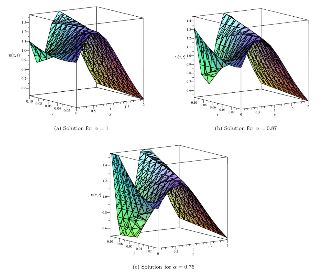
Fig. 1. Surface of $\upsilon (x,t)$ at $\hbar =1$ and n=1. |
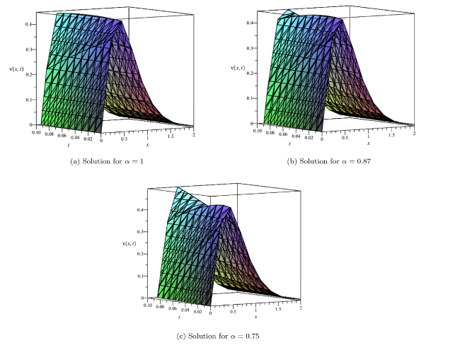
Fig. 2. Surface of $v(x,t)$ at $\hbar =1$ and n=1. |
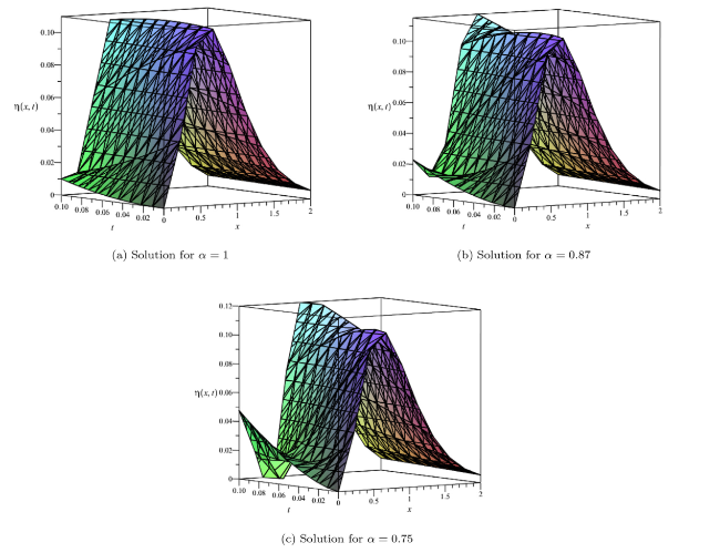
Fig. 3. Surface of $\eta (x,t)$ at $\hbar =1$ and n=1. |
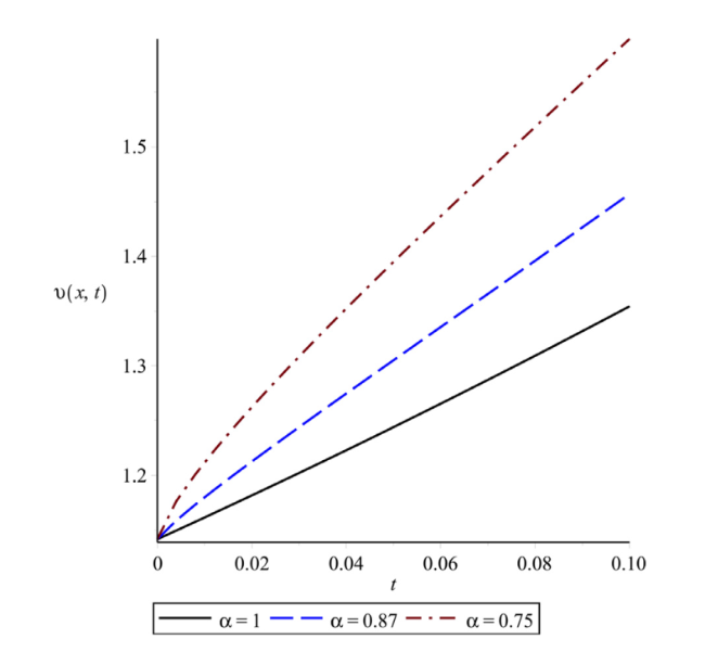
Fig. 4. Plot of solution of $\upsilon (x,t)$ at $\hbar$=−1, n=1 and x=1 for different α with respect to t. |
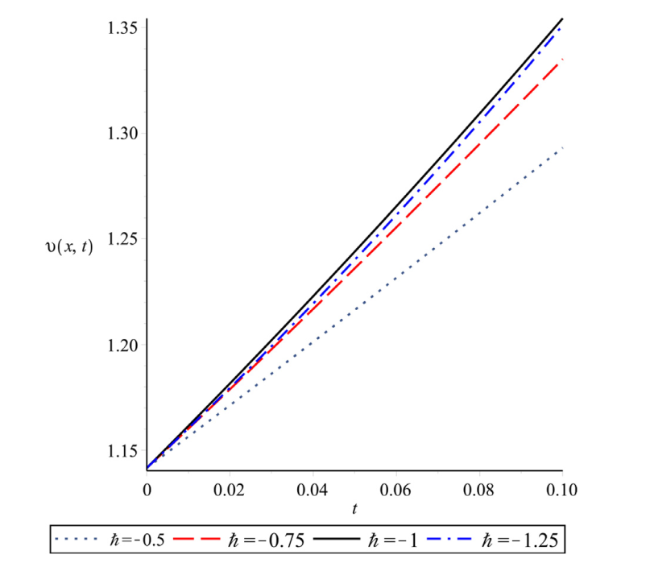
Fig. 5. Plot of solution of $\upsilon (x,t)$ at α=1, n=1 and x=1 for different $\hbar$ with respect to t. |

Fig. 6. Plot of solution of $v(x,t)$ at $\hbar$=−1, n=1 and x=1 for different α with respect to t. |
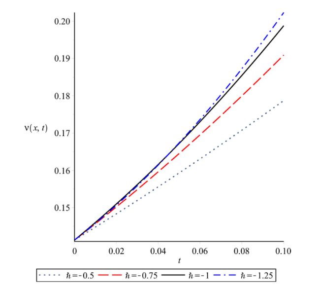
Fig. 7. Plot of solution of $v(x,t)$ at α=1, n=1 and x=1 for different $\hbar$ with respect to t. |
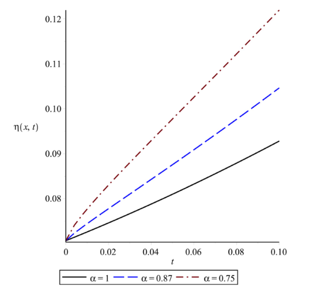
Fig. 8. Plot of solution of $\eta (x,t)$ at $\hbar$=−1, n=1 and x=1 for different α with respect to t. |
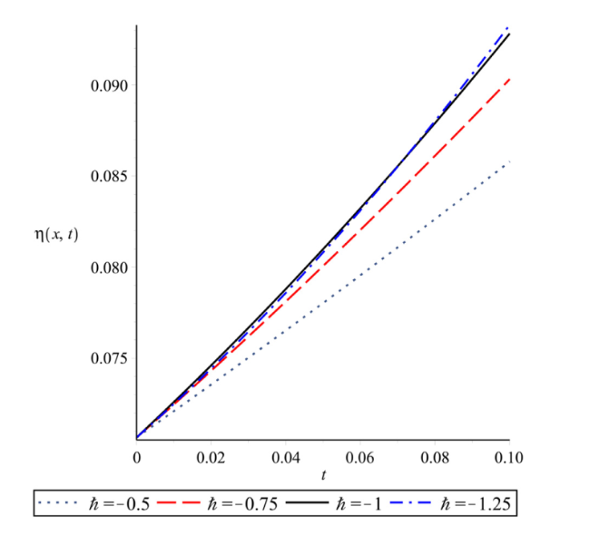
Fig. 9. Plot of solution of $\eta (x,t)$ at α=1, n=1 and x=1 for different $\hbar$ with respect to t. |
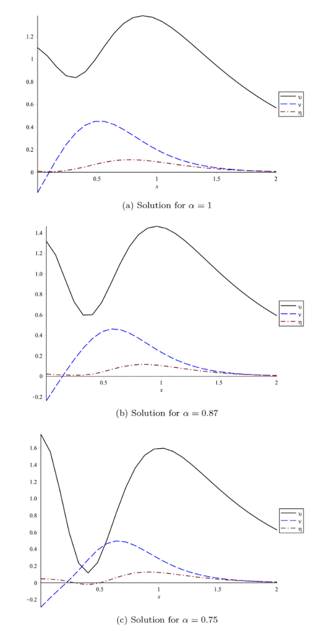
Fig. 10. Plot of $\upsilon (x,t)$, $v(x,t)$ and $\eta (x,t)$ at t=0.1, $\hbar$=−1 and n=1 at different α with respect to x. |
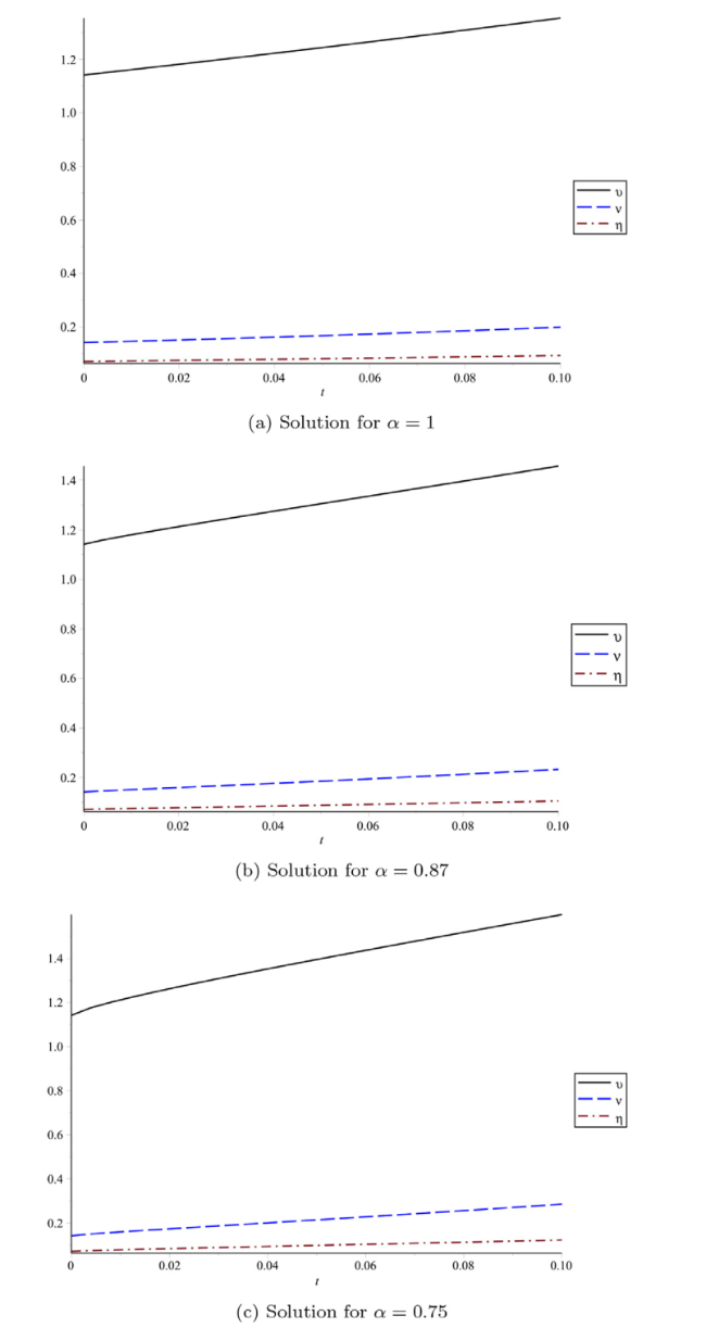
Fig. 11. Plot of $\upsilon (x,t)$, $v(x,t)$ and $\eta (x,t)$ at x=1, $\hbar$=−1 and n=1 at different α with respect to t. |
Table 1. Solution of $\upsilon (x,t)$ for distinct value of $\alpha $ at $\hbar =1$ and n=1. |
| x | t | α=0.75 | α=0.87 | α=1 |
|---|---|---|---|---|
| 0.5 | 0.02 | 1.262280393 | 1.212568783 | 1.181592406 |
| 0.04 | 1.352405802 | 1.274675597 | 1.222863613 | |
| 0.06 | 1.436654239 | 1.335447263 | 1.265422243 | |
| 0.08 | 1.518335351 | 1.396086291 | 1.309268293 | |
| 0.1 | 1.598765045 | 1.457088891 | 1.354401766 | |
| 1.0 | 0.02 | 1.162106447 | 1.234965137 | 1.267846650 |
| 0.04 | 0.9896882900 | 1.149232058 | 1.225829166 | |
| 0.06 | 0.7847083852 | 1.040773233 | 1.170580654 | |
| 0.08 | 0.5521647164 | 0.9113475703 | 1.102101115 | |
| 0.1 | 0.2952822323 | 0.7622188522 | 1.020390547 | |
| 1.5 | 0.02 | 0.8828134901 | 0.8514501594 | 0.8328502944 |
| 0.04 | 0.9427129742 | 0.8902348932 | 0.8574966874 | |
| 0.06 | 1.002007355 | 0.9300372020 | 0.8838101477 | |
| 0.08 | 1.062042570 | 0.9713504106 | 0.9117906749 | |
| 0.1 | 1.123260490 | 1.014337547 | 0.9414382693 |
Table 2. Solution of $v(x,t)$ for distinct value of $\alpha $ at $\hbar =1$ and n=1. |
| x | t | α=0.75 | α=0.87 | α=1 |
|---|---|---|---|---|
| 0.5 | 0.02 | 0.4423886714 | 0.4364455682 | 0.4303802196 |
| 0.04 | 0.4455538582 | 0.4448691506 | 0.4387994896 | |
| 0.06 | 0.4402471169 | 0.4484757711 | 0.4452321518 | |
| 0.08 | 0.4287224660 | 0.4480736325 | 0.4496782061 | |
| 0.1 | 0.4121096499 | 0.4440977454 | 0.4521376526 | |
| 1.0 | 0.02 | 0.1728287613 | 0.1589883142 | 0.1509760603 |
| 0.04 | 0.1998926617 | 0.1760210227 | 0.1615635302 | |
| 0.06 | 0.2273334058 | 0.1938887516 | 0.1730640592 | |
| 0.08 | 0.2555909397 | 0.2127541373 | 0.1854776474 | |
| 0.1 | 0.2847796697 | 0.2326579888 | 0.1988042950 | |
| 1.5 | 0.02 | 0.03498010538 | 0.03263287775 | 0.03126364031 |
| 0.04 | 0.03953634197 | 0.03552589404 | 0.03307457015 | |
| 0.06 | 0.0412220109 | 0.03853996954 | 0.03503090102 | |
| 0.08 | 0.04882049520 | 0.04170561836 | 0.03713263294 | |
| 0.1 | 0.05365491810 | 0.04503141929 | 0.03937976589 |
Table 3. Solution of $\eta (x,t)$ for distinct value of $\alpha $ at $\hbar =1$ and n=1. |
| x | t | α=0.75 | α=0.87 | α=1 |
|---|---|---|---|---|
| 0.5 | 0.02 | 0.08970267542 | 0.09775697313 | 0.1015159448 |
| 0.04 | 0.07104193951 | 0.08822701880 | 0.09668804744 | |
| 0.06 | 0.04918554575 | 0.07642934592 | 0.0905098311 | |
| 0.08 | 0.2460043040 | 0.06252350902 | 0.08298148188 | |
| 0.1 | -0.00241995740 | 0.04662948905 | 0.07410281374 | |
| 1.0 | 0.02 | 0.08302490921 | 0.07776977935 | 0.07460827644 |
| 0.04 | 0.09291657046 | 0.08428742744 | 0.07880429972 | |
| 0.06 | 0.1025589122 | 0.09088689944 | 0.08323889468 | |
| 0.08 | 0.1122128384 | 0.09766350632 | 0.08791206132 | |
| 0.1 | 0.1219709026 | 0.1046517177 | 0.09282379963 | |
| 1.5 | 0.02 | 0.02644106489 | 0.02458075523 | 0.02350237409 |
| 0.04 | 0.03007409727 | 0.02687075129 | 0.02492758007 | |
| 0.06 | 0.03375302765 | 0.02927013356 | 0.02647420159 | |
| 0.08 | 0.03753812679 | 0.03180116880 | 0.02814223865 | |
| 0.1 | 0.04144536717 | 0.03446957201 | 0.02993169123 |
Table 4. Comparison between the solution of q-HAShTM and HAM [20] for $\upsilon (x,t)$, $v(x,t)$ and $\eta (x,t)$ at $\hbar =1$, n=1 and α=1. |
| t | x | $\upsilon (x,t)$ | $v(x,t)$ | $\eta (x,t)$ | |||
|---|---|---|---|---|---|---|---|
| q-HAShTM | HAM | q-HAShTM | HAM | q-HAShTM | HAM. | ||
| 0.02 | 0.2 | 1.10345 | 1.10026 | 0.31350 | 0.31429 | 0.02743 | 0.02692 |
| 0.4 | 1.12217 | 1.22755 | 0.44743 | 0.44903 | 0.083092 | 0.08354 | |
| 0.6 | 1.29362 | 1.29910 | 0.38158 | 0.38186 | 0.10943 | 0.11002 | |
| 0.8 | 1.27512 | 1.27677 | 0.25593 | 0.25545 | 0.099846 | 0.09996 | |
| 1.0 | 1.18159 | 1.18095 | 0.15097 | 0.15052 | 0.07460 | 0.07448 | |
| 0.04 | 0.2 | 1.03947 | 1.02669 | 0.28319 | 0.28633 | 0.02167 | 0.01962 |
| 0.4 | 1.15555 | 1.17863 | 0.44442 | 0.45081 | 0.07582 | 0.07764 | |
| 0.6 | 1.27934 | 1.30162 | 0.39661 | 0.39769 | 0.10788 | 0.11023 | |
| 0.8 | 1.30276 | 1.30933 | 0.27200 | 0.27005 | 0.10311 | 0.10360 | |
| 1.0 | 1.22286 | 1.22029 | 0.16156 | 0.15974 | 0.07880 | 0.07832 | |
Table 5 describes the lower and upper numerical solution of fuzzy $\tilde{\upsilon }(x,t;r,\beta )$, $\tilde{v}(x,t;r,\beta )$ and $\tilde{\eta }(x,t;r,\beta )$ at α=1, r=0.5 with respect to x and t. Table 6 represents the lower and upper numerical solution of fuzzy $\tilde{\upsilon }(x,t;r,\beta )$, $\tilde{v}(x,t;r,\beta )$ and $\tilde{\eta }(x,t;r,\beta )$ at x=0.5, t=0.05 and α=1 with distinct values of r. Fig. 12, Fig. 13, Fig. 14 describe the plot of upper solution(blue) and lower solution(black) of $\tilde{\upsilon }(x,t;r,\beta )$, $\tilde{v}(x,t;r,\beta )$ and $\tilde{\eta }(x,t;r,\beta )$ at α=1, α=0.87 and α=0.75, respectively with respect to r. Fig. 15 represents the surfaces of upper solution(blue) and lower solution(orange) of $\tilde{\upsilon }(x,t;r,\beta )$, $\tilde{v}(x,t;r,\beta )$ and $\tilde{\eta }(x,t;r,\beta )$. Here, Fig. 12, Fig. 13, Fig. 14, Fig. 15 and Table 6 explains that the nature of our unknown functions $\tilde{\upsilon }(x,t;r,\beta )$, $\tilde{v}(x,t;r,\beta )$ and $\tilde{\eta }(x,t;r,\beta )$ are not symmetric even we have taken the coefficient of initial conditions as the symmetric triangular fuzzy number. It is because the nonlinear nature of the system of partial differential equation.
Table 5. Lower and Upper solution of $\tilde{\upsilon }(x,t;r,\beta )$, $\tilde{v}(x,t;r,\beta )$ and $\tilde{\eta }(x,t;r,\beta )$ at $\hbar =1$, n=1 and α=1 and r=0.5. |
| x | t | $\underset{\scriptscriptstyle-}{\upsilon }(x,t;r,0)$ | $\bar{\upsilon }(x,t;r,1)$ | $\underset{\scriptscriptstyle-}{v}(x,t;r,0)$ | $\bar{v}(x,t;r,1)$ | $\underset{\scriptscriptstyle-}{\eta }(x,t;r,0)$ | $\bar{\eta }(x,t;r,1)$ |
|---|---|---|---|---|---|---|---|
| 0.5 | 0.02 | 0.63629 | 1.89413 | 0.31905 | 0.54362 | 0.051686 | 0.14913. |
| 0.04 | 0.62114 | 1.81202 | 0.32272 | 0.55685 | 0.050655 | 0.13669 | |
| 0.06 | 0.60284 | 1.69861 | 0.32599 | 0.56465 | 0.049403 | 0.12015 | |
| 0.08 | 0.58141 | 1.55391 | 0.32885 | 0.56703 | 0.047932 | 0.09952 | |
| 0.11 | 0.55684 | 1.37791 | 0.33131 | 0.56399 | 0.046240 | 0.07479 | |
| 1.0 | 0.02 | 0.58722 | 1.78309 | 0.10954 | 0.19509 | 0.036305 | 0.11496 |
| 0.04 | 0.60397 | 1.85665 | 0.11331 | 0.21593 | 0.037325 | 0.12466 | |
| 0.06 | 0.62104 | 1.93310 | 0.11730 | 0.23914 | 0.038385 | 0.13507 | |
| 0.08 | 0.63843 | 2.01243 | 0.12149 | 0.26473 | 0.039486 | 0.14619 | |
| 0.1 | 0.65614 | 2.0946 | 0.12590 | 0.29269 | 0.040628 | 0.15802 |
Table 6. Lower and Upper solution of $\tilde{\upsilon }(x,t;r,\beta )$, $\tilde{v}(x,t;r,\beta )$ and $\tilde{\eta }(x,t;r,\beta )$ at x=0.5, t=0.05, $\hbar =1$, n=1 and α=1 with different values of r. |
| r | $\underset{\scriptscriptstyle-}{\upsilon }(x,t;r,0)$ | $\bar{\upsilon }(x,t;r,1)$ | $\underset{\scriptscriptstyle-}{v}(x,t;r,0)$ | $\bar{v}(x,t;r,1)$ | $\underset{\scriptscriptstyle-}{\eta }(x,t;r,0)$ | $\bar{\eta }(x,t;r,1)$. |
|---|---|---|---|---|---|---|
| 0 | 1.41246×10⁻⁶ | 2.28732 | 0.21000 | 0.67979 | 3.38205×10⁻⁷ | 0.15335 |
| 0.1 | 0.12431 | 2.18436 | 0.23250 | 0.65629 | 0.01041 | 0.14943 |
| 0.2 | 0.24774 | 2.08004 | 0.25521 | 0.63268 | 0.02064 | 0.14501 |
| 0.3 | 0.37024 | 1.97440 | 0.27811 | 0.60899 | 0.03067 | 0.14011 |
| 0.4 | 0.49180 | 1.86745 | 0.30118 | 0.58524 | 0.04048 | 0.13474 |
| 0.5 | 0.61238 | 1.75923 | 0.32441 | 0.56143 | 0.05005 | 0.12893 |
| 0.6 | 0.73197 | 1.64975 | 0.34777 | 0.53759 | 0.05937 | 0.12268 |
| 0.7 | 0.85054 | 1.53905 | 0.37125 | 0.51374 | 0.06842 | 0.11603 |
| 0.8 | 0.96806 | 1.42715 | 0.39484 | 0.48989 | 0.07718 | 0.10898 |
| 0.9 | 1.08451 | 1.31408 | 0.41852 | 0.46606 | 0.08563 | 0.10155 |
| 1.0 | 1.19985 | 1.19985 | 0.44226 | 0.44226 | 0.09376 | 0.09376 |
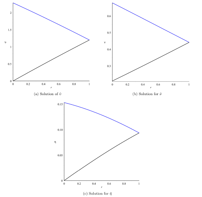
Fig. 12. Plot of $\tilde{\upsilon }(x,t;r,\beta )$, $\tilde{v}(x,t;r,\beta )$ and $\tilde{\eta }(x,t;r,\beta )$ at x=0.5, t=0.05, $\hbar$=−1, n=1, α=1 with respect to r. |
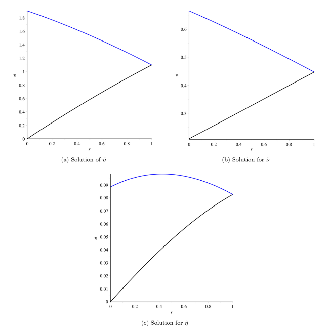
Fig. 13. Plot of $\tilde{\upsilon }(x,t;r,\beta )$, $\tilde{v}(x,t;r,\beta )$ and $\tilde{\eta }(x,t;r,\beta )$ at x=0.5, t=0.05, $\hbar$=−1, n=1, α=0.87 with respect to r. |
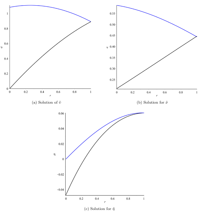
Fig. 14. Plot of $\tilde{\upsilon }(x,t;r,\beta )$, $\tilde{v}(x,t;r,\beta )$ and $\tilde{\eta }(x,t;r,\beta )$ at x=0.5, t=0.05, $\hbar$=−1, n=1, α=0.75 with respect to r. |
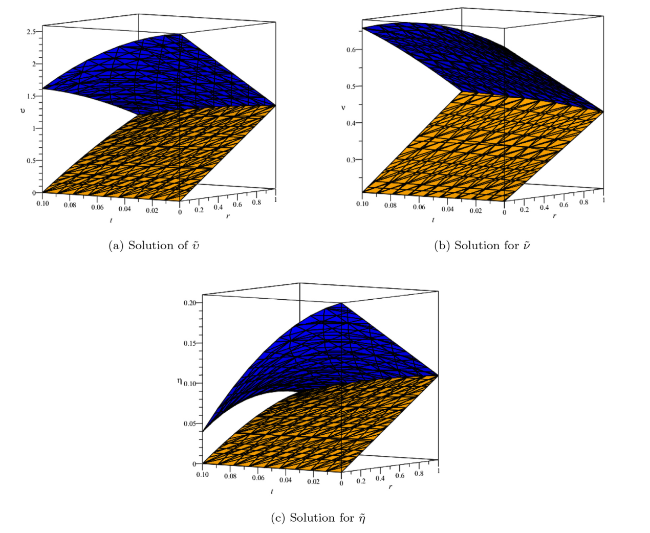
Fig. 15. Surfaces of $\tilde{\upsilon }(x,t;r,\beta )$, $\tilde{v}(x,t;r,\beta )$ and $\tilde{\eta }(x,t;r,\beta )$ at x=0.5, $\hbar$=−1, n=1, α=1. |
8. Conclusion
The fractional and fuzzy-fractional systems of partial differential equation atmospheric internal waves are studied using the analytical approach known as q-HAShTM. A graphical and numerical simulation is provided further to understand the behaviour of the fractional and fuzzy-fractional strategies. The q-HAShTM and HAM comparison explains that the q-HAShTM offers a better solution with faster convergence because the two parameters $\hbar$ and n and fractional approach can be easily solved via q-HAShTM with less complexity because the Shehu transform provides a faster fractional-order solution. The fuzzy-fractional technique has considered the triangular fuzzy number in coefficients of the beginning conditions. The convergent solution for the fuzzy system is provided by q-HAShTM. All of the findings suggest that employing q-HAShTM to understand the behaviour of internal atmospheric waves is beneficial.
Declaration of Competing Interest
The authors declare that they have no known competing financial interests or personal relationships that could have appeared to influence the work reported in this paper.
