
1. Introduction
Nonlinear evolution equations (NLEEs) have sparked a flurry of research articles in establishing a diverse set of solutions for various complex physical models. Several models have been implemented in order to achieve meaningful progress by providing new solutions and simplifying calculations. Among the mathematical approaches used are the Lie symmetry reductions method, Hirota bilinear method, Exp-function method, Darboux transformation method, sine cosine method, modified Ricatti method, Painlev analysis method, Jacobi elliptic function method, generalized exponential rational function method, and various ansatz methods [1], [2], [3], [4], [5], [6], [7], [8], [9], [10], [11], [12], [13], [14], [15], [16], [17], [18], [19], [20], [21], [22], [23], [24], [25], [26], [27], [28], [29], [30], [31], [32]. Solitary waves are a special type of natural ocean phenomenon that is not caused by land movement, lasts only a few seconds, occurs only in a small area, and occurs most frequently far out at sea. Many mathematicians and physicists have been researching ocean physics, marine engineering, acoustics, and hydrodynamics for a long time. Many research works [33], [34], [35], [36], [37], [38], [39], [40], [41], [42] have investigated solitary waves and multiple soliton solutions, particularly the interaction behaviour of travelling waves and dispersive waves, such as trigonometric functions, hyperbolic functions, and exponential functions [43], [44], [45], [46], [47], [48], [49], [50], [51]. In those fields, emphasis has been placed on Burgers-type equations for various wave processes [52], [53], [54], [55], [56], [57]. The Korteweg-de Vries-Burgers equation [52], the Burgers-type equation [53], the (2+1)-dimensional generalized Burgers equation [54], the (2+1)-dimensional coupled Burgers system [55], [56], fractional Burgers-type equations with conformable derivatives [57] and the coupled (2+1)-dimensional Burgers system [58] are some examples of the Burgers type equations. The Burgers system describes the wave propagation processes for nonlinear evolution equations in oceanography, marine engineering, and fluid dynamics, such as nonlinear phenomena in turbulence, diverse non-equilibrium, and interface dynamics.
where and w are three physical wave functions. If we consider w=0, therefore u is independent of z. Hence, Eq. (1) will be transformed to the Burgers equation in (2+1)-dimensions [61], [62]. In ref[63]., to expand on the analysis of Eq (1), the authors adopted the multilinear variable separation approach. In ref[64]., the authors implemented the following prior variable separation approach to invent new soliton solutions to the considered system. Many researchers have recently worked on different dimensions of Burgers systems to obtain analytic and closed-form solutions. In their work, they also show the various wave profiles of the obtained solutions [59], [60], [61], [62], [63], [64]. Alimirzaluo et al. [61] recently studied the (3+1)-dimensional Burgers system using Lie symmetry analysis and constructed 1-, 2-, and 3-dimensional optimal systems. They also obtained a variety of analytical solutions for the system. In this article, an integrable Burgers system (1) will be investigated using two analytical schemes, namely the generalized Kudryashov method and the generalized exponential rational function method. The primary goal of this work is to derive a large number of analytical closed-form solutions to the system (1). In addition, using numerical simulations, we show the different dynamics of wave profiles of some solitary wave solutions in 3D and 2D graphics. However, we believe that the evolutionary dynamics of obtained solitary wave solutions are very interesting and that they are beneficial for complex physical phenomena. The main features of the generalized Kudryashov method and generalized exponential rational function method that will be used in this work are briefly highlighted in the following sections. Both analytical schemes will be summarised in sections 2 and 3. Section 4 depicts several soliton solutions of the Burgers system using two mathematical methods, and various closed-form wave solutions are shown using Wolfram Mathematica, a mathematical software. Section 5 concludes the research study.
2. Generalized kudryashov method
Consider the general form of nonlinear partial differential equations as
P is a polynomial function of in (2). The generalized Kudryashov method describes in the following manner Step 1: Suppose, following is the linear wave transformation on equation
We obtain ordinary differential equation from the equation (2) as
Step 2:The analytic solution of equation (4), we obtain in the given form
where are undefined parameters that will be determined such that ( ) and is the solution of Bernoulli’s differential equation of first order nonlinearity
as it is stated
Step 3: By employing the homogeneous balancing principle on equation (4) to determine the values of M and N.
Step 4: Inserting equation (5) in equation (4) along with (6) and collecting all the coefficient and power of and then equate to zero, we get the set of algebraic equations. After solving the set of equations, with the aid of any suitable mathematical software like Mathematica, Maple, Matlab, the value of the parameters can be determined.
3. Methodology of the GERF method
This section provides a brief explanation of the generalized exponential rational function (GERF) approach for constructing soliton wave solutions to nonlinear PDEs. Consider the following nonlinear partial differential equation
where preserves and its partial derivatives. Ghanbari and Inc [65] introduced this method to generate the exact solitary wave solutions of the NPDEs. The main steps of the GERF method are framed as follows:
Step 1:
To construct numerous analytic solutions, we will use the wave transformations which is mentioned below
where are constants. Now, on inserting equation (9) in (8), we have an ordinary differential equation as follows
where .
Step 2:
Assume that the exact solutions of equation (10) can be expressed as follows
where the value of the positive number N can be calculated by the homogeneous Balancing principle and explicit solution Π(X) is given as
In the above solution, and are real (or complex) numbers which will be computed later.
Step 3: Use equation (11) in (10) along with (12), and considering the combinations of all the coefficients of the same power of and its derivative, and by equating all these coefficients to zero, we obtain the set of algebraic type of equations, and then with the help of any suitable mathematical software like Mathematica, Maple, Matlab, some sets of values of the parameters can be evaluated.
Step 4: Finally, by substituting all the values of the parameters which we obtained in the previous step in equation (11), we will get the required solutions of (1).
4. Soliton solutions to (3+1)-dimensional burgers system
In this part of the manuscript, the exact analytic solutions of the (3+1)-dimensional Burgers system (1) have been determined by using two efficient method: the generalized Kudryashov method and the generalized exponential rational function (GERF) technique.
Using the following transformation in equation (1)
$\begin{aligned}u(x,y,z,t)&=\mathrm{U}(\mathrm{X}),\quad v(x,y,z,t)=\mathrm{V}(\mathrm{X}),\quad w(x,y,z,t)=\mathrm{W}(\mathrm{X})\\\mathrm{where}\quad&X=\kappa\mathrm{~}x+\lambda\mathrm{~}y+\mu\mathrm{~}z-\nu\mathrm{~}t.&\end{aligned}$
Equation (1) reduced in ordinary differential equations which is given as
On simplifying (15), we obtain
where and are integrating constants. Substituting equation (16) in (14), we get
Integrating equation (17) and taking integration constant zero, we have the following reduced equation as
4.1. Implementation of generalized kudryashov method on equation (18)
The homogeneous balancing principle creates the following relationship in order to study a number of closed-form wave solutions and new solitary wave solutions:
where N is a free parameter. Therefore, for any integer N=1, the relation (19) shows that M=2. For specific values of N and M, equation (18) generates the solution stated as
wherein and symbolize the unspecified constants which are to be evaluated. Inserting the solution (20) along with Bernoulli equation (6) in to the equation (18) yields a polynomial in . The following algebraic solutions are developed by collecting the coefficients of similar power of and setting them to zero.
Set 1:
$\begin{aligned}&\delta_0=-\frac{\delta_1}4,\quad\delta_1=\delta_1,\quad\delta_2=-\frac{3 \delta_1}4,\quad\sigma_0=-\frac{\delta_1}{4 \lambda},\quad\sigma_1=\frac{3 \delta_1}{4 \lambda},\\&\nu=-(\kappa^2+\lambda^2+\mu^2+2\kappa K_1+2\mu K_2).\end{aligned}$
Substituting the constant parameters δ0,δ1,δ2,σ0,σ1 and ν in solution (30) first and then in the solution (16), we obtain
As a result of back substitutions, we derive the soliton solution of the system (1) as follows
$\begin{aligned} & u(x, y, z, t)=\frac{\lambda \eta e^{\left(\kappa x+\lambda y+\mu z+\left(\kappa^2+\lambda^2+\mu^2+2 \kappa K_1+2 \mu K_2\right) t\right)}}{1+\eta e^{\left(\kappa x+\lambda y+\mu z+\left(\kappa^2+\lambda^2+\mu^2+2 \kappa K_1+2 \mu K_2\right) t\right)}} \\ & v(x, y, z, t)=K_1+\frac{\kappa \eta e^{\left(\kappa x+\lambda y+\mu z+\left(\kappa^2+\lambda^2+\mu^2+2 \kappa K_1+2 \mu K_2\right) t\right)}}{1+\eta e^{\left(\kappa x+\lambda y+\mu z+\left(\kappa^2+\lambda^2+\mu^2+2 \kappa K_1+2 \mu K_2\right) t\right)}} \\ & w(x, y, z t)=K_2+\frac{\mu \eta e^{\left(\kappa x+\lambda y+\mu z+\left(\kappa^2+\lambda^2+\mu^2+2 \kappa K_1+2 \mu K_2\right) t\right)}}{1+\eta e^{\left(\kappa x+\lambda y+\mu z+\left(\kappa^2+\lambda^2+\mu^2+2 \kappa K_1+2 \mu K_2\right) t\right)}}\end{aligned}$
Set 2:
$\begin{aligned} \delta_{0} & =-\frac{\delta_{1}}{2}, \quad \delta_{1}=\delta_{1}, \quad \delta_{2}=\delta_{0}, \quad \sigma_{0}=\frac{\delta_{0}}{2 \lambda}, \quad \sigma_{1}=-\frac{\delta_{0}}{\lambda} \\ v & =-\left(\kappa^{2}+\lambda^{2}+\mu^{2}+2 \kappa K_{1}+2 \mu K_{2}\right) \end{aligned}$
Substituting the constant parameters and ν in solution (30) first and then in the solution (16), we obtain
$\begin{aligned} \mathrm{U}(X) & =\frac{2 \lambda \eta^{2} e^{2 X}}{-1+\eta^{2} e^{2 X}}, \quad \mathrm{~V}(X)=K_{1}+\frac{2 \kappa \eta^{2} e^{2 X}}{-1+\eta^{2} e^{2} X} \\ \mathrm{~W}(X) & =K_{2}+\frac{2 \mu \eta^{2} e^{2 X}}{-1+\eta^{2} e^{2 X}} \end{aligned}$
As a result of back substitutions, we obtain the breather type soliton solution of the system (1) as follows(22)
$\begin{aligned} & u(x, y, z, t)=\frac{2 \lambda \eta^2 e^{2\left(\kappa x+\lambda y+\mu z+\left(\kappa^2+\lambda^2 \dashv \mu^2+2 \kappa K_1 \dashv 2 \mu K_2\right) t\right)}}{-1+\eta^2 e^{2\left(\kappa x+\lambda y+\mu z z+\left(\kappa^2+\lambda^2+\mu^2+2 \kappa K_1+2 \mu K_2\right) t\right)}}, \\ & v(x, y, z, t)=K_1+\frac{2 \kappa \eta^2 e^{2\left(\kappa x+\lambda y+\mu z+\left(\kappa^2+\lambda^2+\mu^2+2 \kappa K_1+2 \mu K_2\right) t\right)}}{-1+\eta^2 e^{2\left(\kappa x+\lambda y+\mu z+\left(\kappa^2+\lambda^2+\mu^2+2 \kappa K_1+2 \mu K_2\right) t\right)}}, \\ & w(x, y, z t)=K_2+\frac{2 \mu \eta^2 e^{2\left(\kappa x+\lambda y+\mu z+\left(\kappa^2+\lambda^2+\mu^2+2 \kappa K_1+2 \mu K_2\right) t\right)}}{-1+\eta^2 e^{2\left(\kappa x+\lambda y+\mu z+\left(\kappa^2+\lambda^2+\mu^2+2 \kappa K_1+2 \mu K_2\right) t\right)}}.\end{aligned}$
Solution (22) provides the new form of soliton solutions for η=1, and η=3 as follows
$\begin{array}{l} u(x, y, z, t)=\lambda(1+\operatorname{coth}(\kappa x+\lambda y+\mu z-v t)) \\ v(x, y, z, t)=K_{1}+\kappa(1+\operatorname{coth}(\kappa x+\lambda y+\mu z-v t)) \\ w(x, y, z t)=K_{2}+\mu(1+\operatorname{coth}(\kappa x+\lambda y+\mu z-v t)) \end{array}$
$\begin{aligned} & u(x, y, z, t) \\ & =\frac{9 \lambda e^{\kappa x+\lambda y+\mu z-\nu t}}{4 \cosh (\kappa x+\lambda y+\mu z-\nu t)+5 \sinh (\kappa x+\lambda y+\mu z-\nu t)} \\ & v(x, y, z, t) \\ & =K_1+\frac{9 \kappa e^{\kappa x+\lambda y+\mu z-\nu t}}{4 \cosh (\kappa x+\lambda y+\mu z-\nu t)+5 \sinh (\kappa x+\lambda y+\mu z-\nu t)}, \\ & w(x, y, z t) \\ & =K_2+\frac{9 \mu e^{\kappa x+\lambda y+\mu z-\nu t}}{4 \cosh (\kappa x+\lambda y+\mu z-\nu t)+5 \sinh (\kappa x+\lambda y+\mu z-\nu t)}. \\ & \end{aligned}$
Set 3:
$\begin{aligned} \delta_{0} & =0, \quad \delta_{1}=0, \quad \delta_{2}=2 \lambda \sigma_{0}, \quad \sigma_{0}=\sigma_{0}, \quad \sigma_{1}=-2 \sigma_{0} \\ v & =2\left(\kappa^{2}+\lambda^{2}+\mu^{2}-2 \kappa K_{1}-2 \mu K_{2}\right) \end{aligned}$
Substituting the constant parameters meters 𝛿0,𝛿1,𝛿2,𝜎0,𝜎1 and and ν in solution (30) first and then in the solution (16), we obtain
$\begin{matrix} U\left( X \right) = \frac{2\ \lambda }{-1+{{\eta }^{2}}\ {{e}^{2\ X}}},\ \ V\left( X \right)={{K}_{1}}+\frac{2\ \kappa }{-1+{{\eta }^{2}}\ {{e}^{2\ X}}}, \\ W\left( X \right) = {{K}_{2}}+\frac{2\ \mu }{-1+{{\eta }^{2}}\ {{e}^{2\ X}}}. \\ \end{matrix} $
As a result of back substitutions, we derive soliton solution of the system (1) as follows
$\begin{aligned} & u(x, y, z, t) \\ & =\frac{2 \lambda}{-1+\eta^2 e^{2\left(\kappa x+\lambda y+\mu z+\left(\kappa^2+\lambda^2+\mu^2-2 \kappa K_1-2 \mu K_2\right) t\right)}}, \\ & v(x, y, z, t)=K_1 \\ & +\frac{2 \kappa}{-1+\eta^2 e^{2\left(\kappa x+\lambda y+\mu z+\left(\kappa^2+\lambda^2+\mu^2-2 \kappa K_1-2 \mu K_2\right) t\right)}}, \\ & w(x, y, z t)=K_2 \\ & +\frac{2 \mu}{-1+\eta^2 e^{2\left(\kappa x+\lambda y+\mu z+\left(\kappa^2+\lambda^2+\mu^2-2 \kappa K_1-2 \mu K_2\right) t\right)}}. \\ & \end{aligned}$
Set 4:
$\begin{aligned} \delta_{0} & =0, \quad \delta_{1}=0, \quad \delta_{2}=\lambda \sigma_{1}, \quad \sigma_{0}=0, \quad \sigma_{1}=\sigma_{1} \\ \nu & =2\left(\kappa^{2}+\lambda^{2}+\mu^{2}-2 \kappa K_{1}-2 \mu K_{2}\right) . \end{aligned}$
Substituting the constant parameters and ν in solution (30) first and then in the solution (16), we obtain
$\begin{aligned} \mathrm{u}(X) & =-\frac{\lambda}{1+\eta e^{X}}, \quad \mathrm{~V}(X)=K_{1}-\frac{\kappa}{1+\eta e^{X}} \\ \mathrm{~W}(X) & =K_{2}-\frac{\mu}{1+\eta e^{X}} \end{aligned}$
As a result of back substitutions, we acquire the soliton solution of the system (1) as follows
Set 5:
$\begin{array}{l} \delta_{0}=0, \quad \delta_{1}=\delta_{1}, \quad \delta_{2}=\delta_{2}, \quad \sigma_{0}=\sigma_{0}, \quad \sigma_{1}=-\frac{\delta_{2}}{\lambda} \\ \mu=\sqrt{-\kappa^{2}-\lambda^{2}}, \quad v=2\left(-\kappa K_{1}-\sqrt{-\kappa^{2}-\lambda^{2}} K_{2}\right) \end{array}$
Substituting the constant parameters and ν in solution (30) first and then in the solution (16), we obtain
As a result of back substitutions, we obtain the exact solitary wave solution of the system (1) as follows
$\begin{array}{l} u(x, y, z, t) \\ =\frac{\lambda\left(\delta_{2}+\left(1+\eta e^{(\kappa x+\lambda y+\mu z-\nu t)}\right) \delta_{1}\right)}{\left(1+\eta e^{(\kappa x+\lambda y+\mu z-\nu t)}\right)\left(-\delta_{2}+\lambda\left(1+\eta e^{(\kappa x \nmid \lambda y \dashv \mu z-\nu t)}\right) \sigma_{0}\right)}, \\ v(x, y, z, t)=K_{1} \\ \quad+\frac{\kappa\left(\delta_{2}+\left(1+\eta e^{(\kappa x+\lambda y+\mu z-\nu t)}\right) \delta_{1}\right)}{\left(1+\eta e^{(\kappa x+\lambda y+\mu z-\nu t)}\right)\left(-\delta_{2}+\lambda\left(1+\eta e^{(\kappa x+\lambda y+\mu z-\nu t)}\right) \sigma_{0}\right)}, \\ \left.w(x, y, z t)=K_{2}\right) \\ \quad+\frac{\sqrt{-\kappa^{2}-\lambda^{2}}\left(\delta_{2}+\left(1+\eta e^{(\kappa x+\lambda y+\mu z-\nu t)}\right) \delta_{1}\right)}{\left(1+\eta e^{(\kappa x+\lambda y+\mu z-\nu t)}\right)\left(-\delta_{2}+\lambda\left(1+\eta e^{(\kappa x+\lambda y+\mu z-\nu t)}\right) \sigma_{0}\right)}. \end{array}$
Set 6:
$\begin{array}{l} \begin{array}{l} \delta_{0}=\frac{\sigma_{0} \lambda\left(2 \kappa^{2}+2 \lambda^{2}+2 \mu^{2}-\nu-2 \kappa K_{1}-2 \mu K_{2}\right)}{2\left(\kappa^{2}+\lambda^{2}+\mu^{2}\right)}, \\ \delta_{1}= \\ -\frac{\sigma_{0} \lambda\left(2 \kappa^{2}+2 \lambda^{2}+2 \mu^{2}-\nu-2 \kappa K_{1}-2 \mu K_{2}\right)}{\kappa^{2}+\lambda^{2}+\mu^{2}}, \quad \delta_{2}=2 \lambda \sigma_{0}, \\ \sigma_{0}=\sigma_{0}, \quad \sigma_{1}=-2 \sigma_{0} \end{array}\\ \delta_{0}=\frac{\sigma_{0} \lambda\left(2 \kappa^{2}+2 \lambda^{2}+2 \mu^{2}-\nu-2 \kappa K_{1}-2 \mu K_{2}\right)}{2\left(\kappa^{2}+\lambda^{2}+\mu^{2}\right)},\\ \delta_{1}=\\ -\frac{\sigma_{0} \lambda\left(2 \kappa^{2}+2 \lambda^{2}+2 \mu^{2}-\nu-2 \kappa K_{1}-2 \mu K_{2}\right)}{\kappa^{2}+\lambda^{2}+\mu^{2}}, \quad \delta_{2}=2 \lambda \sigma_{0},\\ \sigma_{0}=\sigma_{0}, \quad \sigma_{1}=-2 \sigma_{0} \end{array}$
Substituting the constant parameters , and in solution (30) first and then in the solution (16), we obtain
As a result of back substitutions, we obtain the kink-wave solution of the system (1) as follows
$\begin{aligned} u(x, y, z, t)= & \lambda-\frac{\lambda\left(\nu+2 \kappa K_{1}+2 \mu K_{2}\right)}{2\left(\kappa^{2}+\lambda^{2}+\mu^{2}\right)} \\ & +\frac{2 \lambda}{\eta^{2} e^{2(\kappa x+\lambda y+\mu z-\nu t)}-1}, \\ v(x, y, z, t)= & K_{1}+\kappa-\frac{\kappa\left(\nu+2 \kappa K_{1}+2 \mu K_{2}\right)}{2\left(\kappa^{2}+\lambda^{2}+\mu^{2}\right)} \\ & +\frac{2 \kappa}{\eta^{2} e^{2(\kappa x+\lambda y+\mu z-\nu t)}-1}, \\ w(x, y, z t)= & K_{2}+\mu-\frac{\mu\left(\nu+2 \kappa K_{1}+2 \mu K_{2}\right)}{2\left(\kappa^{2}+\lambda^{2}+\mu^{2}\right)} \\ & +\frac{2 \mu}{\eta^{2} e^{2(\kappa x+\lambda y+\mu z-\nu t)}-1}. \end{aligned}$
For η=1, solution (28) reduces into new form of soliton solution
$\begin{array}{l} u(x, y, z, t) \\ \quad=\frac{\lambda\left(2\left(\kappa^{2}+\lambda^{2}+\mu^{2}\right) \operatorname{coth}(\kappa x+\lambda y+\mu z-\nu t)-2 \kappa K_{1}-2 \mu K_{2}-\nu\right)}{2\left(\kappa^{2}+\lambda^{2}+\mu^{2}\right)}, \\ v(x, y, z, t)=K_{1} \\ \quad+\frac{\kappa\left(2\left(\kappa^{2}+\lambda^{2}+\mu^{2}\right) \operatorname{coth}(\kappa x+\lambda y+\mu z-\nu t)-2 \kappa K_{1}-2 \mu K_{2}-\nu\right)}{2\left(\kappa^{2}+\lambda^{2}+\mu^{2}\right)}, \\ w(x, y, z t)=K_{2} \\ \quad+\frac{\mu\left(2\left(\kappa^{2}+\lambda^{2}+\mu^{2}\right) \operatorname{coth}(\kappa x+\lambda y+\mu z-\nu t)-2 \kappa K_{1}-2 \mu K_{2}-\nu\right)}{2\left(\kappa^{2}+\lambda^{2}+\mu^{2}\right)} \end{array}$
4.2. Implementation of GERF method on equation (18)
For generating solutions, we use balancing principle on highest derivative U′ and nonlinear term in equation (18) which yields that gives N=1.
For the definite values of N=1, the equation (18) generate the solution stated as
where Π(X) is giving by (12). According to the methodology explained in Section 3, we obtain the following closed form solutions of the (3+1)-dimensional Burgers system (1) listed below:
Family 1:
If and , and so expression (12) converts to
Case 1.1
$\begin{aligned} P_{0} & =-\lambda, \quad P_{1}=0, \quad Q_{1}=\lambda, \quad \text { and } \\ v & =2\left(\kappa^{2}+\lambda^{2}+\mu^{2}-\kappa K_{1}-\mu K_{2}\right) \end{aligned}$
Substituting the parameters from equation (31) in solutions (11) and (16), we obtain
$\begin{aligned} U(X) & =-\lambda+\frac{\lambda}{\tanh (X)}, \quad \mathrm{V}(X)=K_{1}-\kappa+\frac{\kappa}{\tanh (X)} \\ \mathrm{W}(X) & =K_{1}-\mu+\frac{\mu}{\tanh (X)} \end{aligned}$
As a result, the examined Burgers system’s soliton solution is achieved
$\begin{array}{l} u(x, y, z, t) \\ = \frac{\lambda}{\tanh \left(\kappa x+\lambda y+\mu z-2\left(\kappa^{2}+\lambda^{2}+\mu^{2}-\kappa K_{1}-\mu K_{2}\right) t\right)} \\ \quad-\lambda, \\ v(x, y, z, t) \\ = \frac{\kappa}{\tanh \left(\kappa x+\lambda y+\mu z-2\left(\kappa^{2}+\lambda^{2}+\mu^{2}-\kappa K_{1}-\mu K_{2}\right) t\right)} \\ \quad+K_{1}-\kappa, \\ w(x, y, z t) \\ \quad+K_{2}-\mu. \end{array}$
Case 1.2
$\begin{aligned} P_{0} & =-\lambda, \quad P_{1}=\lambda, \quad Q_{1}=0, \quad \text { and } \\ \nu & =2\left(\kappa^{2}+\lambda^{2}+\mu^{2}-\kappa K_{1}-\mu K_{2}\right) \end{aligned}$
Substituting the parameters from equation (34) in solutions (11) and (16), we obtain
$\begin{aligned} \mathrm{U}(X) & =\lambda \tanh (X)-\lambda, \quad \mathrm{V}(X)=\kappa \tanh (X)+K_{1}-\kappa, \\ \mathrm{W}(X) & =\mu \tanh (X) K_{1}-\mu . \end{aligned}$
As a result, the examined Burgers system’s soliton solution is achieved
$\begin{aligned} u(x, y, z, t) & =\lambda \tanh (\kappa x+\lambda y+\mu z \\ & \left.-2\left(\kappa^{2}+\lambda^{2}+\mu^{2}-\kappa K_{1}-\mu K_{2}\right) t\right)-\lambda \\ v(x, y, z, t) & =\kappa \tanh (\kappa x+\lambda y+\mu z \\ & \left.-2\left(\kappa^{2}+\lambda^{2}+\mu^{2}-\kappa K_{1}-\mu K_{2}\right) t\right)+K_{1}-\kappa \\ w(x, y, z, t) & =\mu \tanh (\kappa x+\lambda y+\mu z \\ & \left.-2\left(\kappa^{2}+\lambda^{2}+\mu^{2}-\kappa K_{1}-\mu K_{2}\right) t\right)+K_{2}-\mu. \end{aligned}$
Case 1.3
$\begin{aligned} P_{0} & = \pm 2 \lambda, \quad P_{1}=\lambda, \quad Q_{1}=\lambda, \quad \text { and } \\ \nu & =\mp 2\left(2 \kappa^{2}+2 \lambda^{2}+2 \mu^{2}-\kappa K_{1}-\mu K_{2}\right) \end{aligned}$
Substituting the parameters from equation (37) in solutions (11) and (16), we obtain
$\mathrm{U}(X)=\lambda \tanh(X)+\frac{\lambda}{\tanh(X)}\pm2\lambda,\\\mathrm{V}(X)=\kappa \tanh(X)+\frac{\kappa}{\tanh(X)}+K_1\pm2\kappa ,\\\mathrm{W}(X)=\mu \tanh(X)+\frac{\mu}{\tanh(X)}+K_2\pm2\mu.$
As a result, the examined Burgers system’s soliton solution is achieved
$\begin{array}{l} u(x, y, z, t)=\lambda \tanh (\kappa x+\lambda y+\mu z \\ \left.\quad \pm 2\left(2 \kappa^{2}+2 \lambda^{2}+2 \mu^{2}-\kappa K_{1}-\mu K_{2}\right) t\right) \pm 2 \lambda \\ \quad+\frac{\lambda}{\tanh \left(\kappa x+\lambda y+\mu z \pm 2\left(2 \kappa^{2}+2 \lambda^{2}+2 \mu^{2}-\kappa K_{1}-\mu K_{2}\right) t\right)} \\ v(x, y, z, t)=\kappa \tanh (\kappa x+\lambda y+\mu z \\ \left.\quad \pm 2\left(2 \kappa^{2}+2 \lambda^{2}+2 \mu^{2}-\kappa K_{1}-\mu K_{2}\right) t\right)+K_{1} \pm 2 \kappa \\ \quad+\frac{\kappa}{\tanh \left(\kappa x+\lambda y+\mu z \pm 2\left(2 \kappa^{2}+2 \lambda^{2}+2 \mu^{2}-\kappa K_{1}-\mu K_{2}\right) t\right)} \\ w(x, y, z, t)=\mu \tanh (\kappa x+\lambda y+\mu z \\ \left.\quad \pm 2\left(2 \kappa^{2}+2 \lambda^{2}+2 \mu^{2}-\kappa K_{1}-\mu K_{2}\right) t\right)+K_{2} \pm 2 \mu \\ \quad+\frac{\mu}{\tanh \left(\kappa x+\lambda y+\mu z \pm 2\left(2 \kappa^{2}+2 \lambda^{2}+2 \mu^{2}-\kappa K_{1}-\mu K_{2}\right) t\right)} \end{array}$
Case 1.4
Substituting the parameters from equation (39) in solutions (11) and (16), we obtain
As a result, the examined Burgers system’s soliton solution is achieved
$\begin{array}{l} u(x, y, z, t) \\ =P_{0} \\ +P_{1} \tanh \left(\kappa x+\lambda y+\sqrt{-\kappa^{2}-\lambda^{2}} z-2\left(-\kappa K_{1}-\sqrt{-\kappa^{2}-\lambda^{2}} K_{2}\right) t\right) \\ +\frac{Q_{1}}{\tanh \left(\kappa x+\lambda y+\sqrt{-\kappa^{2}-\lambda^{2}} z-2\left(-\kappa K_{1}-\sqrt{-\kappa^{2}-\lambda^{2}} K_{2}\right) t\right)}, \\ v(x, y, z, t) \\ =\frac{\kappa P_{0}}{\lambda} \\ +\frac{\kappa P_{1}}{\lambda} \tanh \left(\kappa x+\lambda y+\sqrt{-\kappa^{2}-\lambda^{2}} z-2\left(-\kappa K_{1}-\sqrt{-\kappa^{2}-\lambda^{2}} K_{2}\right) t\right) \\ +\frac{\kappa Q_{1}}{\lambda \tanh \left(\kappa x+\lambda y+\sqrt{-\kappa^{2}-\lambda^{2}} z-2\left(-\kappa K_{1}-\sqrt{-\kappa^{2}-\lambda^{2}} K_{2}\right) t\right)} \\ +K_{1} \text {, } \\ w(x, y, z, t) \\ =\frac{\sqrt{-\kappa^{2}-\lambda^{2}} P_{1}}{\lambda} \tanh \left(\kappa x+\lambda y+\sqrt{-\kappa^{2}-\lambda^{2}} z-2\left(-\kappa K_{1}-\sqrt{-\kappa^{2}-\lambda^{2}} K_{2}\right) t\right) \\ +\frac{\sqrt{-\kappa^{2}-\lambda^{2}} Q_{1}}{\lambda \tanh \left(\kappa x+\lambda y+\sqrt{-\kappa^{2}-\lambda^{2}} z-2\left(-\kappa K_{1}-\sqrt{-\kappa^{2}-\lambda^{2}} K_{2}\right) t\right)} \\ +\frac{\sqrt{-\kappa^{2}-\lambda^{2}} P_{0}}{\lambda}+K_{2}. \\ \end{array}$
Family 2: Taking and , and so expression (12) converts to
Case 2.1
$\begin{array}{l} P_{1}=0, \quad Q_{1}=-\lambda, \quad \text { and }\\ \nu=-\frac{2}{\lambda}\left(P_{0} \kappa^{2}+P_{0} \lambda^{2}+P_{0} \mu^{2}+\kappa \lambda K_{1}+\lambda \mu K_{2}\right) . \end{array}$
Substituting the parameters from equation (41) in solutions (11) and (16), we obtain
$\begin{array}{l} \mathrm{U}(X)=P_{0}+\frac{\lambda}{\tan (X)}, \quad \mathrm{V}(X)=K_{1}+\frac{\kappa P_{0}}{\lambda}+\frac{\kappa}{\tan (X)} \\ \mathrm{W}(X)=K_{2}+\frac{\mu P_{0}}{\lambda}+\frac{\mu}{\tan (X)} \end{array}$
As a result, the examined Burgers system’s soliton solution is achieved
$\begin{array}{l} u(x, y, z, t)=P_{0} \\ +\frac{\lambda}{\tan \left(\kappa x+\lambda y+\mu z+\frac{2}{\lambda}\left(P_{0} \kappa^{2}+P_{0} \lambda^{2}+P_{0} \mu^{2}+\kappa \lambda K_{1}+\lambda \mu K_{2}\right) t\right)}, \\ v(x, y, z, t)=K_{1}+\frac{P_{0} \kappa}{\lambda} \\ +\frac{\kappa}{\tan \left(\kappa x+\lambda y+\mu z+\frac{2}{\lambda}\left(P_{0} \kappa^{2}+P_{0} \lambda^{2}+P_{0} \mu^{2}+\kappa \lambda K_{1}+\lambda \mu K_{2}\right) t\right)}, \\ w(x, y, z t)=K_{2}+\frac{P_{0} \mu}{\lambda} \\ +\frac{\mu}{\tan \left(\kappa x+\lambda y+\mu z+\frac{2}{\lambda}\left(P_{0} \kappa^{2}+P_{0} \lambda^{2}+P_{0} \mu^{2}+\kappa \lambda K_{1}+\lambda \mu K_{2}\right) t\right)}. \\ \end{array}$
Case 2.2
$\begin{aligned} P_{0} & =i \lambda, \quad P_{1}=\lambda, \quad Q_{1}=0, \quad \text { and } \\ v & =-2 i\left(\kappa^{2}+\lambda^{2}+\mu^{2}-i \kappa K_{1}-i \mu K_{2}\right) \end{aligned}$
Substituting the parameters from equation (44) in solutions (11) and (16), we obtain
$\begin{aligned} \mathrm{u}(X) & =i \lambda-\lambda \tan (X), \quad \mathrm{V}(X)=K_{1}+i \kappa-\kappa \tan (X) \\ \mathrm{W}(X) & =K_{2}+i \mu-\mu \tan (X) . \end{aligned}$
As a result, the examined Burgers system’s soliton solution is achieved
$\begin{aligned} u(x, y, z, t) & =i \lambda-\lambda \tan (\kappa x+\lambda y+\mu z \\ & \left.+2 i\left(\kappa^{2}+\lambda^{2}+\mu^{2}-i \kappa K_{1}-i \mu K_{2}\right) t\right), \\ v(x, y, z, t) & =K_{1}+i \kappa-\kappa \tan (\kappa x+\lambda y+\mu z \\ & \left.+2 i\left(\kappa^{2}+\lambda^{2}+\mu^{2}-i \kappa K_{1}-i \mu K_{2}\right) t\right), \\ w(x, y, z, t) & =K_{2}+i \mu-\mu \tan (\kappa x+\lambda y+\mu z \\ & \left.+2 i\left(\kappa^{2}+\lambda^{2}+\mu^{2}-i \kappa K_{1}-i \mu K_{2}\right) t\right). \end{aligned}$
Case 2.3
Substituting the parameters from equation (47) in solutions (11) and (16), we obtain
As a result, the examined Burgers system’s soliton solution is achieved
$\begin{array}{l} u(x, y, z, t) \\ =P_{0}-\lambda \tan \left(\kappa x+\lambda y+\sqrt{-\kappa^{2}-\lambda^{2}} z\right. \\ \left.+\frac{2}{\lambda}\left(P_{0} \kappa^{2}+P_{0} \lambda^{2}+P_{0} \mu^{2}+\kappa \lambda K_{1}+\lambda \mu K_{2}\right) t\right) \\ +\frac{\lambda}{\tan \left(\kappa x+\lambda y+\mu z+\frac{2}{\lambda}\left(P_{0} \kappa^{2}+P_{0} \lambda^{2}+P_{0} \mu^{2}+\kappa \lambda K_{1}+\lambda \mu K_{2}\right) t\right)}, \\ v(x, y, z, t) \\ =\frac{\kappa P_{0}}{\lambda}-\kappa \tan (\kappa x+\lambda y+\mu z \\ \left.+\frac{2}{\lambda}\left(P_{0} \kappa^{2}+P_{0} \lambda^{2}+P_{0} \mu^{2}+\kappa \lambda K_{1}+\lambda \mu K_{2}\right) t\right) \\ +\frac{\kappa}{\tan \left(\kappa x+\lambda y+\mu z+\frac{2}{\lambda}\left(P_{0} \kappa^{2}+P_{0} \lambda^{2}+P_{0} \mu^{2}+\kappa \lambda K_{1}+\lambda \mu K_{2}\right) t\right)}+K_{1}, \\ w(x, y, z, t) \\ =\frac{\mu P_{0}}{\lambda}-\mu \tan \left(\kappa x+\lambda y+\mu z+\frac{2}{\lambda}\left(P_{0} \kappa^{2}+P_{0} \lambda^{2}\right.\right. \\ \left.\left.+P_{0} \mu^{2}+\kappa \lambda K_{1}+\lambda \mu K_{2}\right) t\right) \\ +\frac{\mu}{\tan \left(\kappa x+\lambda y+\mu z+\frac{2}{\lambda}\left(P_{0} \kappa^{2}+P_{0} \lambda^{2}+P_{0} \mu^{2}+\kappa \lambda K_{1}+\lambda \mu K_{2}\right) t\right)}+K_{2}. \\ \end{array}$
Case 2.4
$\begin{aligned} P_{1} & =\lambda, \quad Q_{1}=-\lambda, \quad \mu=\sqrt{-\kappa^{2}-\lambda^{2}} \text { and } \\ \nu & =2\left(-\kappa K_{1}-\sqrt{-\kappa^{2}-\lambda^{2}} K_{2}\right) . \end{aligned}$
Substituting the parameters from equation (49) in solutions (11) and (16), we obtain
$\begin{array}{c} \mathrm{U}(X)=P_{0}-\lambda \tan (X)+\frac{\lambda}{\tan (X)} \\ \mathrm{V}(X)=K_{1}+\frac{\kappa P_{0}}{\lambda}-\kappa \tan (X)+\frac{\kappa}{\tan (X)} \end{array}$
$\mathrm{W}(X)=K_{2}+\frac{\mu P_{0}}{\lambda}-\mu \tan (X)+\frac{\mu}{\tan (X)}$
As a result, the examined Burgers system’s soliton solution is achieved
$\begin{array}{l} u(x, y, z, t)=P_{0}-\lambda \tan \left(\kappa x+\lambda y+\sqrt{-\kappa^{2}-\lambda^{2}} z\right. \\ \left.\quad-2\left(-\kappa K_{1}-\sqrt{-\kappa^{2}-\lambda^{2}} K_{2}\right) t\right) \\ \quad+\frac{\lambda}{\tan \left(\kappa x+\lambda y+\sqrt{-\kappa^{2}-\lambda^{2}} z-2\left(-\kappa K_{1}-\sqrt{-\kappa^{2}-\lambda^{2}} K_{2}\right) t\right)}, \\ v(x, y, z, t)=\frac{\kappa P_{0}}{\lambda}-\kappa \tan \left(\kappa x+\lambda y+\sqrt{-\kappa^{2}-\lambda^{2}} z\right. \\ \left.\quad-2\left(-\kappa K_{1}-\sqrt{-\kappa^{2}-\lambda^{2}} K_{2}\right) t\right) \\ \quad+\frac{\kappa}{\tan \left(\kappa x+\lambda y+\sqrt{-\kappa^{2}-\lambda^{2}} z-2\left(-\kappa K_{1}-\sqrt{-\kappa^{2}-\lambda^{2}} K_{2}\right) t\right)}+K_{1}, \\ w(x, y, z, t)=\frac{\mu P_{0}}{\lambda}-\mu \tan \left(\kappa x+\lambda y+\sqrt{-\kappa^{2}-\lambda^{2}} z\right. \\ \\ \left.\quad-2\left(-\kappa K_{1}-\sqrt{-\kappa^{2}-\lambda^{2}} K_{2}\right) t\right) \\ \quad+\frac{\mu}{\tan \left(\kappa x+\lambda y+\sqrt{-\kappa^{2}-\lambda^{2}} z-2\left(-\kappa K_{1}-\sqrt{-\kappa^{2}-\lambda^{2}} K_{2}\right) t\right)}+K_{2}. \end{array}$
Family 3:
If and , and so expression (12) converts to
Case 3.1
$\begin{aligned} P_{1} & =2 \lambda, \quad Q_{1}=0, \quad \text { and } \quad v=\frac{2}{\lambda}\left(\kappa^{2}\left(20 \lambda-P_{0}\right)\right. \\ & \left.+\lambda^{2}\left(20 \lambda-P_{0}\right)+\mu^{2}\left(20 \lambda-P_{0}\right)-\lambda\left(\kappa K_{1}+\mu K_{2}\right)\right) \end{aligned}$
Substituting the parameters from equation (51) in solutions (11) and (16), we obtain
As a result, the examined Burgers system’s soliton solution is achieved
$\begin{array}{l} u(x, y, z, t)=\left(P_{0}-20 \lambda\right)+2 \lambda \cot (2(\kappa x+\lambda y+\mu z \\ -\frac{2}{\lambda}\left(\kappa^{2}\left(20 \lambda-P_{0}\right)+\lambda^{2}\left(20 \lambda-P_{0}\right)+\mu^{2}\left(20 \lambda-P_{0}\right)\right. \\ \left.\left.\left.-\lambda\left(\kappa K_{1}+\mu K_{2}\right)\right) t\right)\right), \\ v(x, y, z, t)=K_{1}+\frac{\kappa\left(P_{0}-20 \lambda\right)}{\lambda}+2 \kappa \cot (2(\kappa x+\lambda y+\mu z \\ -\frac{2}{\lambda}\left(\kappa^{2}\left(20 \lambda-P_{0}\right)+\lambda^{2}\left(20 \lambda-P_{0}\right)+\mu^{2}\left(20 \lambda-P_{0}\right)\right. \\ \left.\left.\left.-\lambda\left(\kappa K_{1}+\mu K_{2}\right)\right) t\right)\right), \\ w(x, y, z, t)=K_{2}+\frac{\mu\left(P_{0}-20 \lambda\right)}{\lambda}+2 \mu \cot (2(\kappa x+\lambda y+\mu z \\ -\frac{2}{\lambda}\left(\kappa^{2}\left(20 \lambda-P_{0}\right)+\lambda^{2}\left(20 \lambda-P_{0}\right)+\mu^{2}\left(20 \lambda-P_{0}\right)\right. \\ \left.\left.\left.-\lambda\left(\kappa K_{1}+\mu K_{2}\right)\right) t\right)\right). \end{array}$
Case 3.2
$ P_{0}=3 \lambda, \quad P_{1}=0, \quad Q_{1}=-202 \lambda , and v=-2\left(23 \kappa^{2}+23 \lambda^{2}+23 \mu^{2}+\kappa K_{1}+\mu K_{2}\right) .$
Substituting the parameters from equation (53) in solutions (11) and (16), we obtain
$\begin{aligned} \mathrm{U}(X) & =3 \lambda+\frac{202 \lambda}{10-\cot (2 X)}, \quad \mathrm{V}(X)=K_{1}+3 \kappa+\frac{202 \kappa}{10-\cot (2 X)} \\ \mathrm{W}(X) & =K_{2}+3 \mu+\frac{202 \mu}{10-\cot (2 X)} \end{aligned}$
As a result, the examined Burgers system’s soliton solution is achieved
$\begin{array}{l} u(x, y, z, t)=3 \lambda \\ +\frac{202 \lambda}{\left.10-\cot \left(2 \kappa x+2 \lambda y+2 \mu z+2\left(23 \kappa^{2}+23 \lambda^{2}+23 \mu^{2}+\kappa K_{1}+\mu K_{2}\right) t\right)\right)} \\ v(x, y, z, t) \\ =\frac{202 \kappa}{10-\cot \left(2 \kappa x+2 \lambda y+2 \mu z+2\left(23 \kappa^{2}+23 \lambda^{2}+23 \mu^{2}+\kappa K_{1}+\mu K_{2}\right)\right)}, \\ +K_{1}+3 \kappa \\ w(x, y, z, t) \\ =\frac{202 \mu}{10-\cot \left(2 \kappa x+2 \lambda y+2 \mu z+2\left(23 \kappa^{2}+23 \lambda^{2}+23 \mu^{2}+\kappa K_{1}+\mu K_{2}\right)\right)}, \\ +K_{2}+3 \mu. \end{array}$
Case 3.3
Substituting the parameters from equation (55) in solutions (11) and (16), we obtain
$\begin{aligned} \mathrm{U}(X) & =\left(P_{0}-P_{1} 10\right)+P_{1} \cot (2 X)-\frac{Q_{1}}{10-\cot (2 X)} \\ \mathrm{V}(X) & =K_{1}+\frac{\kappa\left(P_{0}-P_{1} 10\right)}{\lambda}+\frac{\kappa P_{1}}{\lambda} \cot (2 X \\ & -\frac{\kappa Q_{1}}{\lambda(10-\cot (2 X))}, \\ \mathrm{W}(X) & =K_{2}+\frac{\mu\left(P_{0}-P_{1} 10\right)}{\lambda}+\frac{\mu P_{1}}{\lambda} \cot (2 X) \\ & -\frac{\mu Q_{1}}{\lambda(10-\cot (2 X))}. \end{aligned}$
As a result, the examined Burgers system’s soliton solution is achieved
$\begin{array}{l} u(x, y, z, t)=P_{0}-10 P_{1}+P_{1} \cot \left(2 \kappa x+2 \lambda y+2 \sqrt{-\kappa^{2}-\lambda^{2}} z\right. \\ \left.\left.-2\left(-\kappa K_{1}-\sqrt{-\kappa^{2}-\lambda^{2}} K_{2}\right) t\right)\right) \\ +\frac{Q_{1}}{\left.\cot \left(2 \kappa x+2 \lambda y+2 \sqrt{-\kappa^{2}-\lambda^{2}} z-2\left(-\kappa K_{1}-\sqrt{-\kappa^{2}-\lambda^{2}} K_{2}\right) t\right)\right)-10} \text {, } \\ v(x, y, z, t)=\frac{\kappa P_{1}}{\lambda} \cot \left(2 \kappa x+2 \lambda y+2 \sqrt{-\kappa^{2}-\lambda^{2}} z\right. \\ \left.\left.-2\left(-\kappa K_{1}-\sqrt{-\kappa^{2}-\lambda^{2}} K_{2}\right) t\right)\right) \\ +\frac{\kappa Q_{1}}{\left.\lambda \cot \left(2 \kappa x+2 \lambda y+2 \sqrt{-\kappa^{2}-\lambda^{2}} z-2\left(-\kappa K_{1}-\sqrt{-\kappa^{2}-\lambda^{2}} K_{2}\right) t\right)\right)-\lambda} \\ 10 \\ +\frac{\kappa P_{0}}{\lambda}-\frac{10 \kappa P_{1}}{\lambda}+K_{1}, \\ w(x, y, z, t)=\frac{\left(\sqrt{-\kappa^{2}-\lambda^{2}}\right) P_{1}}{\lambda} \cot \left(2 \kappa x+2 \lambda y+2 \sqrt{-\kappa^{2}-\lambda^{2}} z\right. \\ \left.-2\left(-\kappa K_{1}-\sqrt{-\kappa^{2}-\lambda^{2}} K_{2}\right) t\right) \\ +\frac{\sqrt{-\kappa^{2}-\lambda^{2}} Q_{1}}{\left.\lambda \cot \left(2 \kappa x+2 \lambda y+2 \sqrt{-\kappa^{2}-\lambda^{2}} z-2\left(-\kappa K_{1}-\sqrt{-\kappa^{2}-\lambda^{2}} K_{2}\right) t\right)\right)} \\ -\lambda 10 \\ +\frac{\left(\sqrt{-\kappa^{2}-\lambda^{2}}\right)\left(P_{0}-10 P_{1}\right)}{\lambda}+K_{2}. \\ \end{array}$
Family 4:
If and , and so expression (12) converts to
Case 4.1
$\begin{aligned} P_{0} & =2 \lambda, \quad P_{1}=0, \quad Q_{1}=-2 \lambda, \quad \text { and } \\ v & =-\left(\kappa^{2}+\lambda^{2}+\mu^{2}+2 \kappa K_{1}+2 \mu K_{2}\right) \end{aligned}$
Substituting the parameters from equation (57) in solutions (11) and (16), we obtain
$\begin{array}{l} \mathrm{U}(X)=2 \lambda-\frac{2 \lambda\left(1+e^{X}\right)}{\left(1+2 e^{X}\right)}, \quad \mathrm{V}(X)=K_{1}+2 \kappa-\frac{2 \kappa\left(1+e^{X}\right)}{\left(1+2 e^{X}\right)} \\ \mathrm{W}(X)=K_{2}+2 \mu-\frac{2 \mu\left(1+e^{X}\right)}{\left(1+2 e^{X}\right)} \end{array}$
As a result, the examined Burgers system’s soliton solution is achieved
$\begin{array}{c} u(x, y, z, t)=2 \lambda \\ -\frac{2 \lambda\left(1+e^{\left(\kappa x+\lambda y+\mu z+\left(\kappa^{2}+\lambda^{2}+\mu^{2}+2 \kappa K_{1}+2 \mu K_{2}\right) t\right)}\right)}{\left(1+2 e^{\left(\kappa x+\lambda y+\mu z+\left(\kappa^{2}+\lambda^{2}+\mu^{2}+2 \kappa K_{1}+2 \mu K_{2}\right) t\right)}\right)} \\ v(x, y, z, t)=K_{1}+2 \kappa \\ -\frac{2 \kappa\left(1+e^{\left(\kappa x+\lambda y+\mu z+\left(\kappa^{2}+\lambda^{2}+\mu^{2}+2 \kappa K_{1}+2 \mu K_{2}\right) t\right)}\right.}{\left(1+2 e^{\left(\kappa x+\lambda y+\mu z+\left(\kappa^{2}+\lambda^{2}+\mu^{2}+2 \kappa K_{1}+2 \mu K_{2}\right) t\right)}\right)} \\ w(x, y, z t)=K_{2}+2 \mu \\ -\frac{2 \mu\left(1+e^{\left(\kappa x+\lambda y+\mu z+\left(\kappa^{2}+\lambda^{2}+\mu^{2}+2 \kappa K_{1}+2 \mu K_{2}\right) t\right)}\right)}{\left(1+2 e^{\left(\kappa x+\lambda y+\mu z+\left(\kappa^{2}+\lambda^{2}+\mu^{2}+2 \kappa K_{1}+2 \mu K_{2}\right) t\right)}\right.}. \end{array}$
Case 4.2
$\begin{aligned} P_{0} & =-2 \lambda, \quad P_{1}=\lambda, \quad Q_{1}=0, \quad \text { and } \\ \nu & =\left(\kappa^{2}+\lambda^{2}+\mu^{2}-2 \kappa K_{1}-2 \mu K_{2}\right) \end{aligned}$
Substituting the parameters from equation (59) in solutions (11) and (16), we obtain
$\begin{array}{l} \mathrm{U}(X)=\frac{\lambda\left(1+2 e^{X}\right)}{\left(1+e^{X}\right)}-2 \lambda, \quad \mathrm{V}(X)=\frac{\kappa\left(1+2 e^{X}\right)}{\left(1+e^{X}\right)}+K_{1}-2 \kappa \\ \mathrm{W}(X)=\frac{\mu\left(1+2 e^{X}\right)}{\left(1+e^{X}\right)}+K_{2}-2 \mu \end{array}$
As a result, the examined Burgers system’s soliton solution is achieved
$\begin{aligned} u(x, y, z, t) & =\frac{\lambda\left(1+2 e^{\left(\kappa x+\lambda y+\mu z-\left(\kappa^{2}+\lambda^{2}+\mu^{2}-2 \kappa K_{1}-2 \mu K_{2}\right) t\right)}\right)}{\left(1+e^{\left(\kappa x \nmid \lambda y \dashv \mu z-\left(\kappa^{2}+\lambda^{2}+\mu^{2}-2 \kappa K_{1}-2 \mu K_{2}\right) t\right)}\right)} \\ & -2 \lambda, \\ v(x, y, z, t) & =\frac{\kappa\left(1+2 e^{\left(\kappa x+\lambda y+\mu z-\left(\kappa^{2}+\lambda^{2}+\mu^{2}-2 \kappa K_{1}-2 \mu K_{2}\right) t\right)}\right)}{\left(1+e^{\left(\kappa x+\lambda y+\mu z-\left(\kappa^{2}+\lambda^{2}+\mu^{2}-2 \kappa K_{1}-2 \mu K_{2}\right) t\right)}\right)} \\ & +K_{1}-2 \kappa, \\ w(x, y, z, t) & =\frac{\mu\left(1+2 e^{\left(\kappa x+\lambda y+\mu z-\left(\kappa^{2}+\lambda^{2}+\mu^{2}-2 \kappa K_{1}-2 \mu K_{2}\right) t\right)}\right)}{\left(1+e^{\left(\kappa x+\lambda y \dashv \mu z-\left(\kappa^{2}+\lambda^{2} \nmid \mu^{2}-2 \kappa K_{1}-2 \mu K_{2}\right) t\right)}\right)} \\ & +K_{1}-2 \mu. \end{aligned}$
Case 4.3
$\begin{aligned} P_{0} & =-3 P_{1}, \quad Q_{1}=2 P_{1}, \quad \mu=\sqrt{-\kappa^{2}-\lambda^{2}}, \quad \text { and } \\ \nu & =2\left(-\kappa K_{1}-\sqrt{-\kappa^{2}-\lambda^{2}} K_{2}\right) . \end{aligned}$
Substituting the parameters from equation (61) in solutions (11) and (16), we obtain
As a result, the examined Burgers system’s soliton solution is achieved
$\begin{array}{l} u(x, y, z, t) \\ =-3 P_{1}+P_{1} \frac{\left(1+2 e^{\left.\left(\kappa x+\lambda y+\sqrt{-\kappa^{2}-\lambda^{2}} z+2\left(\kappa K_{1}+\sqrt{-\kappa^{2}-\lambda^{2}} K_{2}\right) t\right)\right)}\right.}{\left(1+e^{\left(\kappa x+\lambda y+\sqrt{-\kappa^{2}-\lambda^{2}} z+2\left(\kappa K_{1}+\sqrt{-\kappa^{2}-\lambda^{2}} K_{2}\right) t\right)}\right.} \\ +\frac{2 P_{1}\left(1+e^{\left.\left(\kappa x+\lambda y+\sqrt{-\kappa^{2}-\lambda^{2}} z+2\left(\kappa K_{1}+\sqrt{-\kappa^{2}-\lambda^{2}} K_{2}\right) t\right)\right)}\right.}{\left(1+2 e^{\left.\left(\kappa x+\lambda y+\sqrt{-\kappa^{2}-\lambda^{2}} z+2\left(\kappa K_{1}+\sqrt{-\kappa^{2}-\lambda^{2}} K_{2}\right) t\right)\right)}\right.}, \\ v(x, y, z, t) \\ =K_{1}+\frac{\kappa P_{1}\left(1+2 e^{\left(\kappa x+\lambda y+\sqrt{-\kappa^{2}-\lambda^{2}} z+2\left(\kappa K_{1}+\sqrt{-\kappa^{2}-\lambda^{2}} K_{2}\right) t\right)}\right.}{\lambda\left(1+e^{\left(\kappa x+\lambda y+\sqrt{-\kappa^{2}-\lambda^{2}} z+2\left(\kappa K_{1}+\sqrt{-\kappa^{2}-\lambda^{2}} K_{2}\right) t\right)}\right)} \\ +\frac{2 \kappa P_{1}\left(1+e^{\left(\kappa x+\lambda y+\sqrt{-\kappa^{2}-\lambda^{2}} z+2\left(\kappa K_{1}+\sqrt{-\kappa^{2}-\lambda^{2}} K_{2}\right) t\right)}\right.}{\lambda\left(1+2 e^{\left.\left(\kappa x+\lambda y+\sqrt{-\kappa^{2}-\lambda^{2}} z+2\left(\kappa K_{1}+\sqrt{-\kappa^{2}-\lambda^{2}} K_{2}\right) t\right)\right)}\right.} \\ -\frac{3 \kappa P_{1}}{\lambda} \text {, } \\ w(x, y, z, t)=K_{2} \\ +\frac{\sqrt{-\kappa^{2}-\lambda^{2}} P_{1}\left(1+2 e^{\left(\kappa x+\lambda y+\sqrt{-\kappa^{2}-\lambda^{2}} z+2\left(\kappa K_{1}+\sqrt{-\kappa^{2}-\lambda^{2}} K_{2}\right) t\right)}\right.}{\lambda\left(1+e^{\left.\left(\kappa x+\lambda y+\sqrt{-\kappa^{2}-\lambda^{2}} z+2\left(\kappa K_{1}+\sqrt{-\kappa^{2}-\lambda^{2}} K_{2}\right) t\right)\right)}\right.} \\ +\frac{2 \sqrt{-\kappa^{2}-\lambda^{2}} P_{1}\left(1+e^{\left(\kappa x+\lambda y+\sqrt{-\kappa^{2}-\lambda^{2}} z+2\left(\kappa K_{1}+\sqrt{-\kappa^{2}-\lambda^{2}} K_{2}\right) t\right)}\right.}{\lambda\left(1+2 e^{\left.\left(\kappa x+\lambda y+\sqrt{-\kappa^{2}-\lambda^{2}} z+2\left(\kappa K_{1}+\sqrt{-\kappa^{2}-\lambda^{2}} K_{2}\right) t\right)\right)}\right.} \\ -\frac{3 \sqrt{-\kappa^{2}-\lambda^{2}} P_{1}}{\lambda}. \\ \end{array}$
Family 5:
If and , and so expression (12) converts to
Case 5.1
Substituting the parameters from equation (63) in solutions (11) and (16), we obtain
As a result, the examined Burgers system’s soliton solution is achieved
$\begin{array}{l} u(x, y, z, t) \\ \quad=P_{0}+\frac{Q_{1}}{-2+\tan \left(\kappa x+\lambda y+\sqrt{-\kappa^{2}-\lambda^{2}} z+2\left(\kappa K_{1}+\sqrt{-\kappa^{2}-\lambda^{2}} K_{2}\right) t\right)}, \\ v(x, y, z, t) \\ \quad=K_{1}+\frac{\kappa P_{0}}{\lambda}+\frac{\kappa Q_{1}}{\lambda}\left(-2+\tan \left(\kappa x+\lambda y+\sqrt{-\kappa^{2}-\lambda^{2}} z\right.\right. \\ \left.\left.\quad+2\left(\kappa K_{1}+\sqrt{-\kappa^{2}-\lambda^{2}} K_{2}\right) t\right)\right), \\ w(x, y, z, t) \\ \quad=\frac{\sqrt{-\kappa^{2}-\lambda^{2}} Q_{1}}{\lambda\left(-2+\tan \left(\kappa x+\lambda y+\sqrt{-\kappa^{2}-\lambda^{2}} z+2\left(\kappa K_{1}+\sqrt{-\kappa^{2}-\lambda^{2}} K_{2}\right) t\right)\right)} \\ \quad+K_{2}+\frac{\sqrt{-\kappa^{2}-\lambda^{2}} P_{0}}{\lambda}. \end{array}$
Case 5.2
$ P_{0}=2 \lambda, \quad P_{1}=-\frac{5 \lambda}{4}, \quad Q_{1}=-P_{1}, \quad and v=2\left(\kappa^{2}+\lambda^{2}+\mu^{2}-2 \kappa K_{1}-2 \mu K_{2}\right) .$
Substituting the parameters from equation (65) in solutions (11) and (16), we obtain
As a result, the examined Burgers system’s soliton solution is achieved
$\begin{array}{l} u(x, y, z, t)=2 \lambda-\frac{5 \lambda}{4}(-2+\tan (\kappa x+\lambda y+\mu z \\ \left.\left.-2\left(\kappa^{2}+\lambda^{2}+\mu^{2}+2 \kappa K_{1}+2 \mu K_{2}\right) t\right)\right) \\ \quad+\frac{5 \lambda}{4\left(-2+\tan \left(\kappa x+\lambda y+\mu z-2\left(\kappa^{2}+\lambda^{2}+\mu^{2}+2 \kappa K_{1}+2 \mu K_{2}\right) t\right)\right.}, \\ v(x, y, z, t)=K_{1}+2 \kappa-\frac{5 \kappa}{4}(-2+\tan (\kappa x+\lambda y+\mu z \\ \left.\left.-2\left(\kappa^{2}+\lambda^{2}+\mu^{2}+2 \kappa K_{1}+2 \mu K_{2}\right) t\right)\right) \\ \quad+\frac{5 \kappa}{4\left(-2+\tan \left(\kappa x+\lambda y+\mu z-2\left(\kappa^{2}+\lambda^{2}+\mu^{2}+2 \kappa K_{1}+2 \mu K_{2}\right) t\right)\right.}, \\ w(x, y, z, t)=K_{2}+2 \mu-\frac{5 \mu}{4}(-2+\tan (\kappa x+\lambda y+\mu z \\ \left.\left.-2\left(\kappa^{2}+\lambda^{2}+\mu^{2}+2 \kappa K_{1}+2 \mu K_{2}\right) t\right)\right) \\ \quad+\frac{5 \mu}{4\left(-2+\tan \left(\kappa x+\lambda y+\mu z-2\left(\kappa^{2}+\lambda^{2}+\mu^{2}+2 \kappa K_{1}+2 \mu K_{2}\right) t\right)\right.}. \end{array}$
Case 5.3
$\begin{aligned} Q_{1} & =4 P_{1}\left(1+\frac{P_{1}}{\lambda}\right), \quad \mu=\sqrt{-\kappa^{2}-\lambda^{2}} \quad \text { and } \\ v & =2\left(-\kappa K_{1}-\sqrt{-\kappa^{2}-\lambda^{2}} K_{2}\right) . \end{aligned}$
Substituting the parameters from equation (67) in solutions (11) and (16), we obtain
As a result, the examined Burgers system’s soliton solution is achieved
$\begin{array}{l} u(x, y, z, t)=P_{0}-2 P_{1}+P_{1} \tan \left(\kappa x+\lambda y+\sqrt{-\kappa^{2}-\lambda^{2}} z\right. \\ \left.-2\left(-\kappa K_{1}-\sqrt{-\kappa^{2}-\lambda^{2}} K_{2}\right) t\right) \\ +\frac{4 P_{1}\left(\lambda+P_{1}\right)}{\lambda\left(\tan \left(\kappa x+\lambda y+\sqrt{-\kappa^{2}-\lambda^{2}} z-2\left(-\kappa K_{1}-\sqrt{-\kappa^{2}-\lambda^{2}} K_{2}\right) t\right)-2\right)}, \\ v(x, y, z, t)=K_{1}+P_{0}-\frac{2 P_{1} \kappa}{\lambda}+\frac{P_{1} \kappa}{\lambda} \tan \left(\kappa x+\lambda y+\sqrt{-\kappa^{2}-\lambda^{2}} z\right. \\ \left.-2\left(-\kappa K_{1}-\sqrt{-\kappa^{2}-\lambda^{2}} K_{2}\right) t\right) \\ +\frac{4 \kappa P_{1}\left(\lambda+P_{1}\right)}{\lambda^{2}\left(\tan \left(\kappa x+\lambda y+\sqrt{-\kappa^{2}-\lambda^{2}} z-2\left(-\kappa K_{1}-\sqrt{-\kappa^{2}-\lambda^{2}} K_{2}\right) t\right)-2\right)} \text {, } \\ w(x, y, z, t)=K_{2}+P_{0}-\frac{2 P_{1} \mu}{\lambda}+\frac{P_{1} \mu}{\lambda} \tan \left(\kappa x+\lambda y+\sqrt{-\kappa^{2}-\lambda^{2}} z\right. \\ \left.-2\left(-\kappa K_{1}-\sqrt{-\kappa^{2}-\lambda^{2}} K_{2}\right) t\right) \\ +\frac{4 \mu P_{1}\left(\lambda+P_{1}\right)}{\lambda^{2}\left(\tan \left(\kappa x+\lambda y+\sqrt{-\kappa^{2}-\lambda^{2}} z-2\left(-\kappa K_{1}-\sqrt{-\kappa^{2}-\lambda^{2}} K_{2}\right) t\right)-2\right)}. \\ \end{array}$
Case 5.4
$ P_{0}=(-2+i) \lambda, P_{1}=-\frac{5 \lambda}{4}, \quad Q_{1}=-P_{1}, \quad and v=-2 i\left(\kappa^{2}+\lambda^{2}+\mu^{2}-i \kappa K_{1}-i \mu K_{2}\right) .$
Substituting the parameters from equation (69) in solutions (11) and (16), we obtain
As a result, the examined Burgers system’s soliton solution is achieved
$\begin{array}{l} u(x, y, z, t)=(-2+i) \lambda-\frac{5 \lambda}{4}(-2+\tan (\kappa x+\lambda y+\mu z \\ \left.\left.\quad+2 i\left(\kappa^{2}+\lambda^{2}+\mu^{2}-i \kappa K_{1}-i \mu K_{2}\right) t\right)\right) \\ \quad+\frac{5 \lambda}{4\left(-2+\tan \left(\kappa x+\lambda y+\mu z+2 i\left(\kappa^{2}+\lambda^{2}+\mu^{2}-i \kappa K_{1}-i \mu K_{2}\right) t\right)\right.}, \\ v(x, y, z, t)=K_{1}+(-2+i) \kappa-\frac{5 \kappa}{4}(-2+\tan (\kappa x+\lambda y+\mu z \\ \left.\left.\quad+2 i\left(\kappa^{2}+\lambda^{2}+\mu^{2}-i \kappa K_{1}-i \mu K_{2}\right) t\right)\right) \\ \quad+\frac{5 \kappa}{4\left(-2+\tan \left(\kappa x+\lambda y+\mu z+2 i\left(\kappa^{2}+\lambda^{2}+\mu^{2}-i \kappa K_{1}-i \mu K_{2}\right) t\right)\right.}, \\ w(x, y, z, t)=K_{2}+(-2+i) \mu-\frac{5 \mu}{4}(-2+\tan (\kappa x+\lambda y+\mu z \\ \left.\left.\quad+2 i\left(\kappa^{2}+\lambda^{2}+\mu^{2}-i \kappa K_{1}-i \mu K_{2}\right) t\right)\right) \\ \quad+\frac{5 \mu}{4\left(-2+\tan \left(\kappa x+\lambda y+\mu z+2 i\left(\kappa^{2}+\lambda^{2}+\mu^{2}-i \kappa K_{1}-i \mu K_{2}\right) t\right)\right.}. \end{array}$
Family 6:
If and , and so expression (12) converts to
Case 6.1
$\begin{array}{l} \begin{aligned} P_{0} & =\frac{\lambda\left(4 \kappa^{2}+4 \lambda^{2}+4 \mu^{2}-v-2 \kappa K_{1}-2 \mu K_{2}\right)}{2\left(\kappa^{2}+\lambda^{2}+\mu^{2}\right)}, P_{1}=0 \\ \text { and } Q_{1} & =-5 \lambda . \end{aligned}\\ \end{array}$
Substituting the parameters from equation (71) in solutions (11) and (16), we obtain
$\begin{array}{l} \mathrm{U}(X)=\frac{\lambda\left(4 \kappa^{2}+4 \lambda^{2}+4 \mu^{2}-\nu-2 \kappa K_{1}-2 \mu K_{2}\right)}{2\left(\kappa^{2}+\lambda^{2}+\mu^{2}\right)} \\ -\frac{5 \lambda}{2+\cot (X)}, \\ \mathrm{V}(X)=K_{1}+\frac{\kappa\left(4 \kappa^{2}+4 \lambda^{2}+4 \mu^{2}-\nu-2 \kappa K_{1}-2 \mu K_{2}\right)}{2\left(\kappa^{2}+\lambda^{2}+\mu^{2}\right)} \\ -\frac{5 \kappa}{2+\cot (X)}, \\ \mathrm{W}(X)=K_{1}+\frac{\mu\left(4 \kappa^{2}+4 \lambda^{2}+4 \mu^{2}-\nu-2 \kappa K_{1}-2 \mu K_{2}\right)}{2\left(\kappa^{2}+\lambda^{2}+\mu^{2}\right)} \\ -\frac{5 \mu}{2+\cot (X)}. \end{array}$
As a result, the examined Burgers system’s soliton solution is achieved
$\begin{aligned} u(x, y, z, t) & =\frac{\lambda\left(4 \kappa^{2}+4 \lambda^{2}+4 \mu^{2}-\nu-2 \kappa K_{1}-2 \mu K_{2}\right)}{2\left(\kappa^{2}+\lambda^{2}+\mu^{2}\right)} \\ & -\frac{5 \lambda}{2+\cot (\kappa x+\lambda y+\mu z-\nu t)}, \\ v(x, y, z, t) & =K_{1}+\frac{\kappa\left(4 \kappa^{2}+4 \lambda^{2}+4 \mu^{2}-\nu-2 \kappa K_{1}-2 \mu K_{2}\right)}{2\left(\kappa^{2}+\lambda^{2}+\mu^{2}\right)} \\ w(x, y, z, t) & =\frac{5 \kappa}{2+\cot (\kappa x+\lambda y+\mu z-\nu t)}, \\ & -\frac{\mu\left(4 \kappa^{2}+4 \lambda^{2}+4 \mu^{2}-\nu-2 \kappa K_{1}-2 \mu K_{2}\right)}{2\left(\kappa^{2}+\lambda^{2}+\mu^{2}\right)} \\ & \end{aligned}$
Case 6.2
$\begin{array}{l} P_{0}=-\frac{\lambda\left(4 \kappa^{2}+4 \lambda^{2}+4 \mu^{2}+v+2 \kappa K_{1}+2 \mu K_{2}\right)}{2\left(\kappa^{2}+\lambda^{2}+\mu^{2}\right)} \\ P_{1}=q, \text { and } Q_{1}=0 \end{array}$
Substituting the parameters from equation (73) in solutions (11) and (16), we obtain
$\begin{aligned} \mathrm{U}(X) & =\lambda(2+\cot (X)) \\ - & \frac{\lambda\left(4 \kappa^{2}+4 \lambda^{2}+4 \mu^{2}-\nu-2 \kappa K_{1}-2 \mu K_{2}\right)}{2\left(\kappa^{2}+\lambda^{2}+\mu^{2}\right)}, \\ \mathrm{V}(X) & =K_{1}+\kappa(2+\cot (X)) \\ - & \frac{\kappa\left(4 \kappa^{2}+4 \lambda^{2}+4 \mu^{2}-\nu-2 \kappa K_{1}-2 \mu K_{2}\right)}{2\left(\kappa^{2}+\lambda^{2}+\mu^{2}\right)}, \\ \mathrm{W}(X) & =K_{2}+\mu(2+\cot (X)) \\ - & \frac{\mu\left(4 \kappa^{2}+4 \lambda^{2}+4 \mu^{2}-\nu-2 \kappa K_{1}-2 \mu K_{2}\right)}{2\left(\kappa^{2}+\lambda^{2}+\mu^{2}\right)}. \end{aligned}$
As a result, the examined Burgers system’s soliton solution is achieved
$\begin{aligned} u(x, y, z, t) & =\lambda(2+\cot (\kappa x+\lambda y+\mu z-\nu t)) \\ & -\frac{\lambda\left(4 \kappa^{2}+4 \lambda^{2}+4 \mu^{2}-\nu-2 \kappa K_{1}-2 \mu K_{2}\right)}{2\left(\kappa^{2}+\lambda^{2}+\mu^{2}\right)}, \\ v(x, y, z, t) & =K_{1}+\kappa(2+\cot (\kappa x+\lambda y+\mu z-\nu t)) \\ & -\frac{\kappa\left(4 \kappa^{2}+4 \lambda^{2}+4 \mu^{2}-\nu-2 \kappa K_{1}-2 \mu K_{2}\right)}{2\left(\kappa^{2}+\lambda^{2}+\mu^{2}\right)}, \\ w(x, y, z, t) & =K_{2}+\mu(2+\cot (\kappa x+\lambda y+\mu z-\nu t)) \\ & -\frac{\mu\left(4 \kappa^{2}+4 \lambda^{2}+4 \mu^{2}-\nu-2 \kappa K_{1}-2 \mu K_{2}\right)}{2\left(\kappa^{2}+\lambda^{2}+\mu^{2}\right)}. \end{aligned}$
Case 6.3
Substituting the parameters from equation (75) in solutions (11) and (16), we obtain
As a result, the examined Burgers system’s soliton solution is achieved
$\begin{array}{l} u(x, y, z, t)=P_{0}+2 \lambda+\lambda \cot \left(\kappa x+\lambda y+\sqrt{-\kappa^{2}-\lambda^{2}} z\right. \\ \left.+2\left(\kappa K_{1}+\sqrt{-\kappa^{2}+\lambda^{2}} K_{2}\right) t\right) \\ +\frac{Q_{1}}{\left(2+\cot \left(\kappa x+\lambda y+\sqrt{-\kappa^{2}-\lambda^{2}} z+2\left(\kappa K_{1}+\sqrt{-\kappa^{2}+\lambda^{2}} K_{2}\right) t\right)\right)}, \\ v(x, y, z, t)=K_{1}+\frac{\kappa P_{0}}{\lambda}+2 \kappa+\kappa \cot \left(\kappa x+\lambda y+\sqrt{-\kappa^{2}-\lambda^{2}} z\right. \\ \left.+2\left(\kappa K_{1}+\sqrt{-\kappa^{2}+\lambda^{2}} K_{2}\right) t\right) \\ +\frac{\kappa Q_{1}}{\lambda\left(2+\cot \left(\kappa x+\lambda y+\sqrt{-\kappa^{2}-\lambda^{2}} z+2\left(\kappa K_{1}+\sqrt{-\kappa^{2}+\lambda^{2}} K_{2}\right) t\right)\right)}, \\ w(x, y, z, t)=K_{2}+\frac{\mu P_{0}}{\lambda}+2 \mu+\mu \cot \left(\kappa x+\lambda y+\sqrt{-\kappa^{2}-\lambda^{2}} z\right. \\ \left.+2\left(\kappa K_{1}+\sqrt{-\kappa^{2}+\lambda^{2}} K_{2}\right) t\right) \\ +\frac{\mu Q_{1}}{\lambda\left(2+\cot \left(\kappa x+\lambda y+\sqrt{-\kappa^{2}-\lambda^{2}} z+2\left(\kappa K_{1}+\sqrt{-\kappa^{2}+\lambda^{2}} K_{2}\right) t\right)\right)}. \\ \end{array}$
5. Graphical illustration of some soliton solutions
This section is focused on providing us with the dynamical behavior of the newly revealed solutions, including various types of hyperbolic functions, rational functions, and trigonometric functions, through various forms to represent a more clear picture of the dynamical wave profiles of the (3+1)-dimensional Burgers system using Mathematica 11.3. These solutions are determined by using two different methods, such as the generalized Kudryashov method and the generalized exponential rational function method, which are novel and distinct from previous findings in the literature and are computed by other mathematical techniques for the same equation given. Three-dimensional and two-dimensional wave profiles are two distinct wave structures that are more beneficial and useful for investigating various forms of unique and secure analytic solutions, including several free independent parameters. Using appropriate choices of involved free constant parameters, different solitary wave profiles, such as multi-wave solitons, singular soliton, elastic behavior of multi-wave peakon solitons, kink wave profiles, and other types of gained solutions, are produced. In Figs. 1-7, we depicted the dynamical behavior of the graphics for several derived solutions and then described the dynamics of the provided wave profiles.
Fig. 1: The dynamical form of the analytic solutions u,v and w for the equation (21) shows soliton wave profiles. These soliton wave structures have been recorded by choosing suitable values of parameters and is approved for numerical simulation. Moreover, two-dimensional wave profiles show kink wave propagation along the x-axis at y=−2,1, and y=2.
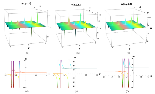
Fig. 1. The prospective view of solitons described by equation (21) describes for related parameter values and . 2D graph plot for . |
Fig. 2: This figure demonstrates the three-graphical structures of the obtained solution (22) with respect to time t. Different multiple soliton wave profiles have been observed. The figure is sketched for the appropriate value of parameters and t=0.01. The dynamics of wave propagation along the x-axis are investigated at .
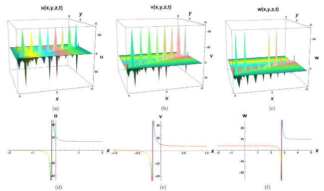
Fig. 2. The prospective view of breather-wave solitons described by equation (22) describes for related parameter values and t=0.01. |
Fig. 3: The wave profiles for the solution (28) are presented in this figure. The single peakon wave profiles have been observed for the suitable value of parameters and t=1. The wave propagation profiles of the wave along the x-axis are shown in the Figs. 3(e), 3(d), and 3(f) at y=−1,0.3, and y=2.
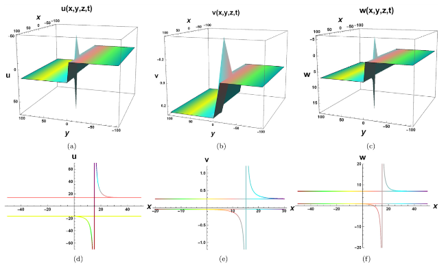
Fig. 3. The prospective view of interactions between one soliton with kink waves described by equation (28) describes for related parameter values $\kappa=0.151, \quad \lambda=15, \quad \mu=$ $3, v=12, \eta=5, K_{1}=0.12, K_{2}=4.2, z=1.2, y=-10.3,2$ and t=1. |
Fig. 4: This figure strongly shows three distinct wave forms of the solutions u,v and w for equation (48) with the suitable values of parameters and t=0.871. Furthermore, 2D wave profiles are illustrated in this figure along the x-axis for parameter y = −3,9. By analyzing the expressions of the multisoliton and periodic oscillations have been considered for the value of random parameters.
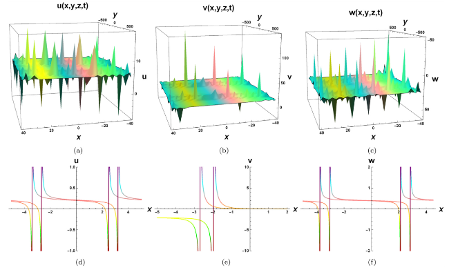
Fig. 4. The prospective view of localized interactions of diverse solitons described by equation (43) describes for related parameter values and t=0.871. 2D plot for y=−3,9. |
Fig. 5: In this figure, the localized wave structures of the multisoliton wave profiles have been investigated for the solutions u,v and w for the equation (54) via 3D and 2D plots. The dynamics of wave propagation along the x-axis are investigated at y=2. The graphical demonstration shows that the multisoliton wave profiles keep their velocities, shapes and amplitudes invariant during the appropriate value of parameters and t=0.5.
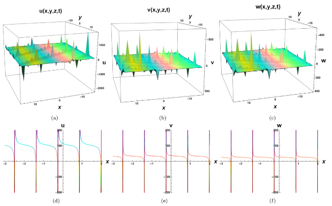
Fig. 5. The prospective view of singularity-form solitary waves described by equation (54) describes for related parameter values and t=0.5. |
Fig. 6: The graphical depiction of the obtained solutions u,v and w for the equation (58) are represented via a three-dimensional plot with respect to time t. The kink wave profile has been observed for the appropriate value of parameters and t=0.31. Moreover, two-dimensional wave profiles show kink wave propagation along the x-axis at y=−3,−1, and y=1.
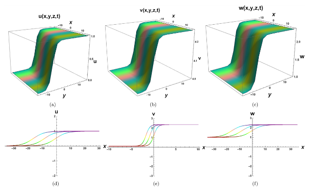
Fig. 6. The prospective view of kink-form waves described by equation (58) describes for related parameter values and t=0.31. 2D plot for y=−3,−1,1. |
Fig. 7 : The evolutionary dynamics of the solutions u,v and w for the equation (58) are visualized graphically in this figure via three dimensional plots. We have recorded the elastic behavior of the distinct solitary wave profiles. These figures are sketched by considering the suitable values of parameters and t=0.23. The wave propagation of the shapes is shown via two-dimensional plot along the x-axis at y=4.

Fig. 7. The prospective view of new solitary waves described by equation (66) describes for related parameter values and t=0.23. 2D graph plot for y=4. |
6. Conclusion
In this paper, we investigated the (3+1)-dimensional Burger’s system analytically to derive more general and newly formed exact solitary wave solutions of different kinds, such as trigonometric and hyperbolic functions, rational functions, and semi-rational functions. We have successfully used two analytical mathematical methods, the generalized Kudryashov (GK) method and the generalized exponential rational function (GERF) method, to construct a rich variety of exact closed-form solutions under various family cases. We also demonstrated our newly established solutions graphically with the assistance of Wolfram Mathematica by choosing suitable best values for the constant parameters. These complex soliton solutions are more useful and helpful in the future in the advanced research and development of dynamics of solitons, fluid dynamics, nonlinear dynamics, telecommunications, industrial studies, hydrodynamics, and several other areas of mathematical physics and nonlinear sciences. It is remarkable to notify that the implemented techniques have been established as productive, promising, and simple mathematical tools for dealing with any NLEEs that arise in ocean engineering, marine physics, plasma physics, and other engineering disciplines using the GK and GERF methods. We believe that the achieved various soliton solutions will be useful in explaining the rich dynamical wave profiles in soliton theory and ocean engineering.
Declaration of Competing Interest
The authors declare that they have no known competing financial interests or personal relationships that could have appeared to influence the work reported in this paper.
Acknowledgment
The first author, Sachin Kumar, has received the research grant for this work which is supported and funded by SERB-DST, India, under project scheme EEQ/2020/000238.
