
1. Introduction
The most critical stage in shipbuilding is its design stage in ship engineering [1], [2]. The ship designer must consider all technical requirements from the shipowners as well as the performance requirements comprehensively [3]. The whole ship design process is a very complex process. When processing a ship design process, what designers often encounter are complex design steps and massive workloads. In detail, the whole design process can be divided into five steps, including concept design, initial design, basic design, detail design, and manufacturing design. Each design stage has its purpose. For instance, in the conceptual design stage, the ship’s specifications and purpose need to be determined, while in the preliminary design, the hull form needs to be determined. Since the hull shape form has a decisive influence on the ship’s sailing performance and seakeeping performance, the initial design is a very critical design stage e.g. [4].
The initial ship hull design [5] is a process of designing and evaluating hull forms to determine the final optimal hull structure, with the objective to achieve the best hydrodynamic performances. The design process of the hull form is a try-and-error or cyclic process. Designers usually need to select an initial hull model to avoid a heavy modeling process. Based on the initial hull model, designers can obtain the optimal solutions by looping over geometry modification and performance evaluation [6]. The hull form design process may require a large workload and cost much time and resources, which depends not only on the hull modification but also on the performance evaluation cost. After designers choose a set of geometric parameters for a possible new hull, the designer must evaluate the hydrodynamic/hydrostatic performance of the ship hull. Take resistance calculation as an example: the Computational Fluid Dynamics (CFD) calculations, e.g. [7], often may cost several hours or even a whole day, not to mention the modeling time cost. Thus, in order to shorten the time required for the hull form design, the best choice is to reduce the workload of the geometric modification process and the calculation process.
The objective of the ship performance evaluation process is to evaluate the performance of the designed hull form. Therefore, if we can use a more effective method to evaluate the performances of the hull form, the time required for hull design can be significantly shortened and less dependent on the designers’ experiences. Often time, it is just impossible to go through all the possible design scenariosbecause of the time or the limitation of designers’ experience. However, if we are able to find the mappings of all possible hull forms in the design space to the resistance value, we may further simplify and optimize the hull form design process in the largest possible design space, and hence when designers designed a new hull form, they can immediately find the relationship between the ship performance and ship hull geometric shape, saving much time, labor, experience, and cost. Then, the question is how to find the complete mapping between various hull forms and their performances. The mapping relation between the hull form and its performance is complicated, nonlinear, and non-intuitive in general. The first reason is that more than hundreds and even thousands of parameters are required to describe a ship hull form, which leads to the complexity of the mapping. The second reason is that this mapping relation is implicitly embedded in a super-manifold with thousands of dimensions, requiring many different implicit representations to describe such mapping relation, if it is explainable and rationalizable. Even if it may be explainable, it may still be difficult for us to obtain an explicit mathematical model that can meet the design accuracy requirements.
Deep Learning (DL) technology, in particular the deep neural network (DNN) [8], is a class of artificial intelligence-based machine learning methods [9]. DNN is a powerful method, which has complex network structures and multiple layers of artificial neural networks. In some cases, DNN can outperform human expert analysis and performance. Recently, not limited to the computer science where it was initially located, DL technology has successfully applied in other fields, including computer vision, audio processing, natural language processing, and search engines. The main advantage of DL technology is that it enables machines to improve their decision process based on both data as well as machine experience. Furthermore, in the past few years, DL technology has become one of the most versatile and efficient tools for handling classification and regression tasks [10], [11].
As a powerful machine learning tool, DL technology can extract the complicated relationship between input data and output data by feeding a DL model with a sample dataset e.g. [12], [13]. Through the training process, the trained DL model can use the uncovered hidden relationship to make predictions. Thus, DL technology is very suitable for dealing with the task that needs to deduce the mapping between two vectors since it allows a DL model to learn from the sample dataset and deduce the mapping relationships.
In some recent studies, based on DL technology, some researchers have used data-driven approaches to solve many problems in naval architecture engineering. Representatively, Milaković et al. [14] developed a machine learning-based method for predicting ship speed profile in a complex ice field under the situation that computational methods have difficulties capturing the entire complexity of the ship-ice interaction process. Wackers et al. [15] used a machine learning approach to reduce the computational effort of CFD simulations. Meanwhile, there have been many researches adopting DL technology to aid engineering design due to its convenience. For instance, Gunpinar et al. [16] adopted regression/neural network methods to establish a design support system for car side silhouette design. Shaeffer et al. [17] used a machine learning approach to regress existing data to obtain a model to assist the early-stage of the hull form design.
In current literature, most reported researches use the principal dimensions of the hull as the input parameters of ANN to forecast its performance. For instance, Cepowski et al. [18] established a DL model to estimate added resistance of ships based on the principal dimensions of the hull. Grabowska et al. [19] forecast realized the prediction of hull’s resistance based on parameters with the highest influence by adopting DL models. However, in the initial design stage, both the principal dimensions and the hull surface should be a design target, which is rarely considered in the current application of DL technology in hull design. A DL model which can only conduct the relationship between the principal dimensions of the hull and its performances cannot satisfy the ship designer’s requirements.
With the rapid developments of artificial intelligence technology, it is possible to use DL-based machine learning methods to efficiently obtain the mapping relationship between any hull form in the design space and the performance results required in the performance evaluation stage by revealing the inner relationships of a sample dataset. In detail, following the ideas of DL technology, we need to prepare a dataset that contains a suitable amount of samples located in the designers-required design space to show mapping style between hull forms and corresponding evaluated performance, which will be further used to train the DL model. After establishing the dataset, we can establish an FCNN model with correct hyperparameters to ensure the model is suitable for the current mission, analyze and reveal internal mapping relationships between hull form and corresponding performance, and store the relationships in the model for further use. Once the results predicted by the DL model are close enough to the actual result to satisfy design requirements, then designers can adopt it to evaluate the performances in real-time, which will save the workload in the design loop process.
Simply put, the application of DL technology in ship engineering to assist the ship design can be treated as transforming the ship design process into a ship selection process, making sure designers can immediately finish the performance evaluation process after they finish the geometry modification process to get the hull form. The main reason for using DL technology-based method rather than other machine learning methods is that DL technology-based machine learning method has high accuracy and good adaptability to very complicated problems, especially for an object like a hull form, a very complex object, which will need many parameters to express a complete hull form. Based on DL technology, we can create a large enough model to discover the mapping relationships among all parameters used to describe a ship hull form and its hydrodynamic performance.
In this work, we have developed a Deep Learning Neural Network model for the initial design of ship hulls. In specific, we construct a Fully Connected Neural Network (FCNN) model to predict and evaluate the total resistance for hull form based on geometry modification parameters, which can forecast not only the performance of hulls with different principal dimensions but also the performance of hulls with different hull forms. We believe the DL model establishment process in this work provides an effective and practical solution to assist the hull form at its initial design stage. It is noted that the data-driven design method proposed in this work aims to save ship designers’ workload and time cost in the initial design stage. Compared with other design-assistant methods, such as structural optimization methods [20], [21], by adopting the method proposed in this paper, ship designers can immediately find the suitable or optimal hull shape and hence the hydrodynamics/hydrostatic performance of hulls by adjusting the geometry modification parameters. However, this method sacrifices the calculation accuracy and ignores the inner structure, making it only suitable to be used in the initial design stage.
The paper is organized as follows. In the rest of the paper, we first briefly introduce the method of expressing the hull form as geometry modification parameters. We then outline the process for gathering the required sample data to train the deep learning model before demonstrating the trained DL model, followed by the detailed process about the hyperparameters tuning process and model training process. Next is followed by several examples demonstrating how to use the proposed deep learning model to predict the total resistance of hull structures. Specifically, based on several forms of hull structures located in design space rather than in the sample dataset, we compare the prediction result of the deep learning model with the evaluation result of the potential flow method. Through these cases, we seek to demonstrate that the deep learning technology-based prediction method proposed in this work can accurately predict the hull form performance based on a set of geometry modification parameters, and hence assisting the hull form design process.
2. Geometry modification expression method
2.1. Free-form deformation (FFD)
Free-Form Deformation (FFD) is a geometric modification technique mainly used to deal with the deformation of rigid objects. Sederberg and Parry developed FFD in 1986 [22], where they used the ternary tensor product Bernstein polynomial control a Bézier volume in space. In FFD, all the deformation processes happened in a local parametric normalized coordinate system, which follows Eq. (1), whose boundary is the lattice space.
· - the origin of the lattice coordinate system,
· - the edge vectors along the axes of the local coordinate system (S,T,U),
· - coordinate values in the local coordinate system, lies in (0,1) for any point located at the interior of the lattice space.
All control points are attached to the pre-defined lattice coordinate system, with an artificially determined distribution independent of the shape of the rigid object. An evenly distributed control point was adopted here, which is also the most commonly used distribution. In the even distribution, the lattice space will be divided into l plane, m planes, and n planes in the direction of s-axis, t-axis, and u-axis, respectively, where the intersection point of every three planes constitutes a control point. The relationship between the global coordinate system and the lattice coordinate system can be seen in Fig. 1. Eq. (2) shows the position of control point P in the lattice space, which is formed by the intersection of the ith plane on the s-axis, the jth plane on the t-axis, and the kth plane on the u-axis,

Fig. 1. The relationship between the global coordinate system and the lattice coordinate system. |
The position of all rigid object points will be changed based on the total influence from all the control points, where the influence weight is inversely proportional to the distance the object point and the control point. Taking the object point P as an example, we show the relationship between the position after deformation and the initial position in Eq. (3),
· - the transformation from real space to lattice space,
· - the inverse transformation from lattice space to real space,
· - Bernstein polynomials,
· - the initial position of the point.
As shown in Eq. (3), due to the characteristics of the Bézier polynomials, the influence weight of a control point to an object point will change based on the distance, which leads that with the increase of the distance, the influence weight of the control point to the object point decreases quickly, making a control point can only significant modify nearby part of the object. The characteristic of distance determines the influence weight of the control point ensures that one can adjust the shape of the object more intuitively.
The application of FFD used in this work is based on the PyGem framework [23], which is a python library using Free-Form Deformation (FFD), Radial Basis Functions (RBF), and Inverse Distance Weighting (IDW) to parametrize and morph complex geometries.
2.2. Geometry modification process of hull form
In the hull form design process, designers usually select an initial hull form model and modify the initial model to find a new hull form to avoid a massive modeling process. In this paper, we select the hull form of the KRISO Container Ship (KCS), which was developed by the Korean Maritime and Ocean Engineering Research Institute (KMOERI), as the initial hull form. To facilitate the accuracy verification of the calculation program used to generate samples in the dataset, the hull form used in this paper is a 1:31.6 scale model. As one of the most commonly used ship models, KCS has been used as benchmarks for many calculation methods for its structure, lines plan, and model test results are open to the public. Table 1 shows the basic geometric parameters of the scaled KCS hull form model used in this paper.
Table 1. Basic geometric parameters of the initial hull form model. |
| Geometric parameters | Scaled hull model |
|---|---|
| Length between perpendiculars | 7.279 m |
| Breadth | 0.703 m |
| Draft | 0.342 m |
| Wetted surface area | 9.438 m2 |
| Design speed | 2.196 m/s |
In this work, we use the right-handed coordinate system to describe the hull form model and its deformation range, where the x-axis parallel with the hull length direction and the y-axis parallel with the hull width direction. Fig. 1 shows the hull structure position in a fixed coordinate system. Consider that a hull is a symmetrical object, we only consider half of the hull model in order to reduce the number of geometry modification parameters, which will decrease half the number of geometry modification parameters. In this work, we selected the hull in the negative direction of the y-axis as the geometry modification object, which can be done by doing a mirroring process to obtain the complete hull model.
In this work, the geometry modification process of hull form has been transformed into a set of geometry modification parameters by combining the linear transformation method and the FFD technique. In detail, the linear transformation method was adopted to adjust the principal dimensions and sailing speed of the hull form model, and the FFD technique was adopted to modify the geometry shape of the hull form, which leads to two kinds of geometry modification parameters. The geometry modification process of hull form in this paper has been divided into three sub-stages for more effortless intuitive operation.
We called the first sub-stage of the geometry modification process the hull stretch stage, where only the length, width, and height will be changed. Suppose that the initial hull model has been transformed to a hull point set , whose density is dense enough to make the result predicted by the calculation method used satisfies the engineering requirements. Then the relationship between the intermediate hull point set after the first sub-stage and the initial hull point set is shown in Eq. (4).
where:
- the position of the ith hull point of the initial model,
- the total number of points used to present hull form model,
- length change rate, breadth change rate, and height change rate.
After finishing the first sub-stage of the geometry modification process, we continue with the second sub-stage of the geometry modification process, which is responsible for changing the draft of the hull structure model. The relationship between the intermediate hull point set $ \mathscr{S}_{I}$ after the second sub-stage and the intermediate hull point set $ \mathscr{S}_{e}$ after the first sub-stage are given as follows,
$ \mathscr{S}_{I}=\mathscr{S}_{e}+\alpha_{z} \cdot \alpha_{d} \cdot\left[\begin{array}{ccc} 0 & 0 & D_{o} \\ & \vdots & \\ 0 & 0 & D_{o} \\ & \vdots & \\ 0 & 0 & D_{o} \end{array}\right]$
where:
- the draft change rate,
- the draft of the initial hull form model.
At the third sub-stage of the geometry modification process, we adjust hull form shape based on the FFD technique on the intermediate hull point set . Since FFD deforms the object based on the control points attached to the lattice coordinate system, and only the object point inside the lattice space can be modified, we need to determine the shape and position of the lattice space with the intermediate hull point set to ensure every hull point located inside the lattice space. Meanwhile, all hull samples in the dataset have different principal dimensions that lead to the position, and the size of the lattice space for each sample is different and needs to be determined in a fixed mode for data validity. The lattice form chosen in this work is a parallelepiped lattice space, which is appropriate for a slender object like ship hull model, and it is more convenient to be adopted in real design process, In this work, we use the extreme coordinate value of the intermediate hull point set to get the position and the size of the lattice space for easy operation, where we compare all hull points inside it to obtain the maximum and minimum coordinate values on each axis separately. Assume that the maximum coordinate value of all points in a hull structure in the xyz coordinates are , , , and the minimum coordinate value of all points in the hull structure are , , . We can then obtain the length , breadth , and height of the parallelepiped lattice space as follows,
where:
- gap rates in the 𝑥, 𝑦, 𝑧 directions,
⊙- the element multiplication.use
As shown in Eq. (6), we added three different gap rates in the x, y, and z directions to ensure the entire hull model can be completely enclosed inside the lattice space. Besides, the position of the origin of the lattice space in the hull coordinate system is also related to the extreme coordinate value of hull points, which follows Eq. (7).
The control point layout adopts in this work is an even distribution, which is the commonly used distribution and suitable for the parallelepiped lattice. For the lattice volume that is constructed based on the extreme coordinate value of hull points, the parallelepiped lattice should also be a slender body with a long length and a relatively short breadth and height. Due to the shape feature of the lattice space, the number of control points in the length direction should be much larger than the number of control points in the other two directions so that the geometry modification can be more reasonable and the geometry modification results become abundant. In FFD, the movements of control points are measured based on the lattice coordinate system, whose actual movements in the hull coordinate system are related to the size of the lattice space, which gives us the advantage to set up the range of all control points without attention to the difference of the principal dimensions of hull structures. We created a finite-size lattice volume of control points based on the initial lattice space to do the geometry modification, whose current position of all control points in the hull coordinate system was represented by matrix Λ. Finally, as shown in Eq. (8), based on FFD, we can obtain the final hull point set based on the lattice space and the position matrix Λ of the lattice of control points,
where:
FFD - FFD operation.
The entire geometry modification process of the hull form is shown in Fig. 2. The geometry modification method adopted in this paper provides an excellent way to summarize the whole geometry modification process with a smaller number of representative parameters which can represent the hull form modified from the KCS hull model. In this work, the geometry modification parameters used to express the hull form include length change rate, breadth change rate, height change rate, draft change rate, and the movement amount of all control points. By modifying the principal dimension modification parameters, we can change the principal dimensions of the final hull model, and by modifying the movement amount of control points, we can change the final hull form.

Fig. 2. Entire geometry modification process of the hull form. |
2.3. Various measures to prevent irrational hull models
Since training a DL model requires a large dataset, it will take much time to generate the dataset by manually changing the deformation parameters. Although the new hull model generated by artificially changing the deformation parameters can make the dataset more intuitive, it is difficult for the artificially generated hull dataset to cover the entire deformation space. Moreover, when the designer artificially changes the deformation parameters to generate a new hull model, the designer will give more consideration to the hull model that he or she considers reasonable due to the designer’s subjective influence. Considering the above reasons, we use random distribution functions to randomly change the deformation parameters to specify the ship hull’s deformation. Randomly changing the deformation parameters will save time and ensure that the generated dataset elements can be distributed as evenly as possible in the entire deformation space. However, since we will randomly change all deformation parameters and the generated dataset is large, irrational hull forms will inevitably appear during the hull generation process. Moreover, if we ignore these irrational hulls, this will cause the finally trained DL model’s prediction accuracy to decrease. To avoid the appearance of irrational hulls, we have taken several measures to avoid irrational hulls.
The possibility of generating irrational hulls can be reduced by adopting different truncated normal distributions and setting different standard deviations. However, due to the need to generate many hull models, there is no guarantee that irrational hulls will not appear after deformation. After analyzing the irrational hull we generated, we found that three reasons mainly cause the irrational hulls. The first and the most important reason is that the hull points are very close to or even crossing the XoZ plane. When the control point approaches the XoZ plane, the hull point will also approach the XoZ plane. When the hull point is very close to the XoZ plane or even crosses the XoZ plane to the area where , the width of a particular hull area will be very small or even become a negative value. From an engineering perspective, the hull at this time is irrational. The second reason is that the distance between the hull points after deformation is too large. When the distance between the hull points is too large, the panel area will be too large, which will cause the accuracy of the calculation result of the panel method to decrease. The third reason is that the local deformation of the hull is too large. Specifically, when a particular area of the hull has an immense change and other areas have small deformations, the calculation core based on the potential flow theory may not handle such a hull. Even if it can, the result will be inaccurate.
When the hull point of a hull is too close to the XoZ plane or crosses the XoZ plane to the area where , then that hull will not meet the engineering requirements and become irrational. The hull points being too close to or crossing the XoZ plane are caused by the preset control points’ offset range. The offset range of the control point determines the hull’s deformation space, and a sufficiently large offset range of the control point can ensure that the hull also has a large enough deformation space. To reduce the DL model’s training time, when setting the control point offset range, we will compress the control point offset range as much as possible while ensuring that the deformation space is large enough. In this paper, the offset range of the control point will change according to its location. Specifically, the control points near the bow and stern will have a more extensive offset range, while the control points near the parallel middle body of the hull will have a smaller offset range. We give different offset ranges for the control points in different regions to reflect our different degrees of emphasis on different regions. By giving the control points close to the bow and stern a more extensive offset range, we ensure that the hull’s bow and stern part have a more extensive deformation range. Since the hull surfaces at the bow and stern of the KCS are more complex and have large varying curvatures, the more extensive offset range makes the hull points near the bow and stern more likely to be too close to or crossing the XoZ plane. When generating the dataset, most of the irrational hulls are caused by the hull points being too close to or crossing the XoZ plane. Even if only one hull point approaches or crosses the XoZ plane, the deformed hull is irrational. If we do not take any measures to avoid such errors, there will be many invalid elements in the dataset. To solve this kind of error, we correct the Y coordinate value of the hull point to ensure that it will not be too close to or cross the XoZ plane. In this way, we can avoid such errors and obtain a thinner hull without irrational hull conditions. Eq. (9) expresses the relationship between the hull point after correction and the hull point before correction.
$ \begin{array}{l} \overline{x_{i}}=x_{i} \\ \overline{y_{i}}=\left\{\begin{array}{ll} y_{i}, & y_{i} \leq y_{s} \\ y_{s} \cdot e^{-a\left(y_{i}-y_{s}\right)}, & y_{i}>y_{s} \end{array}\right. \\ \overline{z_{i}}=z_{i} \text { on } \quad i=1, \ldots, h \end{array}$
where:
are ith hull point coordinates before correction,
are ith hull point coordinates after correction,
is small constant for decide boundary,
a is correction rate.
As shown in Eq. (9), we use the constant to determine whether a hull point being too close to or crossing the XoZ plane. Since the Y-coordinate values of all hull points are negative, if the Y-coordinate value of a hull point is less than , then the hull point has enough distance from the XoZ plane, which is acceptable to us. On the contrary, when the Y-coordinate value of a hull point is greater than , the hull point is too close to the XoZ plane, which will not meet the requirements we set in advance. When the Y-coordinate value of a hull point is greater than , we will correct the hull point. Eq. (9) is equivalent to setting a repelling point for each hull point, which ensures that the closer the hull point is to the repelling point, the greater the rejection.
The second reason for the appearance of an irrational hull is that the distance between the hull points after deformation is too large. When the distance between the hull points of the deformed hull is too large, the panel’s size will be too large, making the calculation accuracy decrease. Unlike when the hull points are too close or crossing the XoZ plane, which violates the engineering requirements, the hull with a too large distance between the hull points does not violate the engineering requirements. The existence of hulls with too large distances between hull points will make the accuracy of the dataset elements inconsistent, which will affect the prediction accuracy of the final DL model. We need to ensure that the accuracy of the elements in the dataset is roughly the same. A DL model trained based on a dataset with roughly the same element accuracy can predict the correct change trend of the hydrodynamic results with the change of deformation parameters and guide the design. Simultaneously, excessive local deformation of the hull may also lead to a decrease in calculation accuracy, so we also need to avoid this type of hull.
To prevent an irrational hull from appearing in the dataset, we need to determine that the deformation of a ship hull is reasonable every time when we generated a new hull. In this work, we determine whether the deformation of a ship hull is too large or the distance between the hull points is too large by judging the change in the distance between the hull points before and after the deformation. As shown in Eq. (10), suppose that a hull model contains total h hull points, then we first define a matrix to show the distance between each hull point and the k other hull points closest to it in the hull before FFD deformation.
After performing FFD deformation, we can obtain a new matrix based on U, and then we can define the new matrix as . The matrix V shown in Eq. (11) reflects the distance between the hull point and the other k hull points closest to it (based on the hull before the deformation) after deformation.
Based on matrix U and matrix V, we can base on Eq. (12) to get the deformed hull’s distance change rate matrix named .
After we obtain a new hull form, we can determine whether the new hull’s local deformation is too large or the distance between hull points is too large according to the matrix W. First, we stipulate that the maximum element in the matrix W, i.e. , is not greater than a constant τ that we set in advance. Second, we stipulate that the standard deviation of all matrix W elements is not greater than the constant ψ we set in advance. Therefore, in general, judging whether the new hull is reasonable or not depends on whether or not the matrix W satisfies the conditions posted in Eq. (13),
$\begin{array}{l} W_{\max } \leq \tau \\ \text { and } s_{W} \leq \psi \end{array}$
Adjusting parameter τ can ensure that the distance between adjacent hull points will not increase excessively, therefore ensuring that the panel area will not become too large. While adjusting parameter ψ ensures that the entire hull will not have sizeable local deformation. If the new hull matrix W does not satisfy these two conditions in Eq. (13), we will deem the new hull as an irregular or irrational hull form. After several attempts, we can choose a control parameter group with smaller values, which leads to a high pass rate for generating ship hull form. Table 2 shows the two preset parameters used to prevent the appearance of irrational hulls.
Table 2. Two parameters used to prevent the appearance of irrational hulls. |
| Parameters | Actual values |
|---|---|
| τ | 2.0 |
| ψ | 0.8 |
3. Data collection
3.1. Hull performance acquisition method
One sample in the dataset needs to contain hull form and corresponding performances to provide input and output to the DL model. All methods that can acquire the performance of the hull form can be adopted. The acquisition method can be a performance evaluation method to calculate the performance of each sample in the dataset or a collection method to collect existing samples to avoid computational work. The sample collection method is not suitable for the acquisition method used here since this paper’s unique geometry modification method. We can use many calculation methods to evaluate the performance of the hull form, from the high-precision CFD method based on Navier-Stokes to the potential flow method based on assumptions.
The choice of calculation method depends on the design stage and design purpose assisted by the DL model. In detail, because designers need to determine the principal dimensions and hull form of the ship in the initial design stage, the design space in the initial design stage will be larger than that in other design stages, which leads to the dataset for training the DL model who guides the initial design should contain more hull samples. It will cause colossal computing time when using the high-fidelity CFD method to establish a dataset containing many samples. In contrast, designers need minor and precise modifications to the hull form in the detail design stage, making the DL model that guides the detail design needs a dataset with low number requirement but high precision samples.
The purpose of the DL model established in this paper is to assist the hull design process, which belongs to the initial design stage, and because of the need to predict the performance of hull models with different main sizes and hull forms, it has a larger design space. Simultaneously, since the hull model needs to be rechecked and fined at several design stages after the initial design, the accuracy of the evaluation results in the initial design stage is lower compared with subsequent design stages, making the potential flow method can satisfy the accuracy requirement. To sum up, in this work, we choose the potential flow method as the hull performance acquisition method to calculate the performance of each sample. The role of CFD simulations in this work is generating data and establishing the dataset to tune and train the neural network model. The hull model of each sample in the dataset is generated by randomly adjusting the geometry modification parameters, and the total resistance of each sample in the dataset is evaluated based on the CFD method.
3.2. The total resistance calculation theory
To reduce the computational workload when constructing the dataset, we treat the resistance performance of the hull as the only evaluation indicator. The resistance performance of the hull is one of the most critical factors when designers evaluate the hull form, which will directly or indirectly affect many performances of the ship, including but not limited to design speed, engine horsepower, and fuel consumption. Considering the verification purpose of the proposed method, only the situation that the ship hull sailing in still water has been considered.
The total resistance of a ship sailing in still water consists of many sources, including wind, hull surface, and ship appendages. According to the simplification guideline provided by the International Towing Tank Conference (ITTC) [24], the total resistance was decomposed as frictional resistance and wave-making resistance . In this paper, we adopt the classical ITTC frictional resistance formula [24] to calculate the frictional resistance and adopt Dawson’s method [25] to calculate the wave-making resistance. The classic ITTC friction resistance formula plays a vital role in resistance estimation, with the accuracy that can satisfy engineering requirements when dealing with most ship types, which follows Eq. (15).
$ C_{f}=\frac{0.075}{(\lg R e-2)^{2}}$
where:
·ρ - density of water,
·U - constant speed,
·S - wetted surface area,
· - friction coefficient,
· - Reynolds number.
Since Dawson’s method has high calculation efficiency, the wave-making resistance calculation based on it usually only needs a few minutes to complete one calculation case. Meanwhile, due to its lower CPU requirements, Dawson’s method-based computation code can be run in parallel computations in a personal computer. In Dawson’s method, the total flow ψ is assumed to be the composition of double-body flow ϕ and wavy flow φ, as follows,
The double-body potential flow and wavy flow satisfy different boundary conditions: the double-body flow must satisfy the boundary conditions on the hull surface, while the wavy flow must satisfy the boundary conditions on both the hull surface and the free surface. After twice expansions based on the Taylor series, the free surface condition can be written as follows,
$ \begin{array}{l} \begin{array}{l} \phi_{x}\left(\phi_{x} \varphi_{x}+\phi_{y} \varphi_{y}\right)_{x}+\phi_{y}\left(\phi_{x} \varphi_{x}+\phi_{y} \varphi_{y}\right)_{y} \\ \quad+\frac{1}{2} \varphi_{x}\left(\phi_{x}^{2}+\phi_{y}^{2}\right)_{x}+\frac{1}{2} \varphi_{y}\left(\phi_{x}^{2}+\phi_{y}^{2}\right)_{y}+g \varphi_{z} \\ \quad-\phi_{z z}\left(\phi_{x} \varphi_{x}+\phi_{y} \varphi_{y}\right)=\frac{1}{2} \phi_{z z}\left(\phi_{x}^{2}+\phi_{y}^{2}-U^{2}\right) \\ \quad-\frac{1}{2} \phi_{x}\left(\phi_{x}^{2}+\phi_{y}^{2}\right)_{x}-\frac{1}{2} \phi_{y}\left(\phi_{x}^{2}+\phi_{y}^{2}\right)_{y} \end{array}\\ \text { on } z=0 \text { free surface. } \end{array}$
where:
·g - acceleration of gravity,
·U - constant advance speed of the ship.
The total resistance computation program used in this work is an in-house computer code developed by the authors’ laboratory [26], which is based on the classic ITTC friction resistance formula and the Dawson method. The validation and the accuracy of the method can be found in the previous works, e.g. [26], [27]. The in-house computer code can be run in parallel in a personal computer, further shortening the calculation time to establish the dataset.
3.3. Design space of samples in the dataset
The final valid space for the prediction of the DL model depends entirely on the design space of the samples in the dataset. The larger the design space of the sample, the wider the effective space of the final DL model, which also means that more samples are needed to train the DL model. Since in this paper, we have represented the geometry modification process of the hull model into a set of geometry modification parameters, the design space of all samples depends on the variation range of geometry modification parameters.
Moreover, we expand the design space by adding speed parameters to the sample to help designers further reduce the workload in the initial design stage. Each sample in the dataset has a different sailing speed, which means the final DL model will also have the ability to predict the total resistance of the hull model under different Froude numbers. As shown in Eq. (18), the sailing speed also has been transformed to a speed parameter, just like the geometry modification parameters.
where:
· - actual Froude number,
· - initial Froude number,
· - Froude number change rate.
As shown in Table 3, we first set the range of principal dimension modification parameters, including length change rate, breadth change rate, height change rate, draft change rate, and Froude number change rate, which determines the design space of the hull model specification. In this paper, we set the variable range of length change rate, breadth change rate, and height change rate can be changed from 0.8 to 1.2. Moreover, since the draft of the ship will be changed drastically considering the different situations of fully loaded and unloaded, we have given a range of the draft change rate to simulate the unloaded condition, which can be changed from −0.4 to 0. Further, the Froude number change rate can be changed from 0.7 to 1.3.
Table 3. The variation range of part of the deformation parameter. |
| Geometry modification parameter | Variable range |
|---|---|
| $α_{x}$ | [0.8,1.2] |
| $α_{y}$ | [0.8,1.2] |
| $α_{z}$ | [0.8,1.2] |
| $α_{d}$ | [−0.4,0] |
| $α_{f}$ | [0.7,1.3] |
The number of control points determines the fineness of the geometry modification of the hull form. The more control points, the finer the geometric modification of the hull form. In this work, we created a (20×4×6) lattice of control points, where exist 20 control points on the x-axis, 4 control points on the y-axis, and 6 control points on the z-axis. As shown in Table 4, we pre-defined the parameters used to determine the lattice space.
Table 4. Parameters used to determine the lattice space. |
| Parameters | x-axis | y-axisn | z-axis |
|---|---|---|---|
| Offset rate | 0.05 | 0.05 | 0.05 |
| Rotation angle | 0.0 | 0.0 | 0.0 |
| N control points | 20 | 4 | 6 |
All control points are evenly distributed in the lattice space, moving freely in three axis directions. To avoid unreasonable hull forms and reduce the number of the geometric modification parameters, we select different fixed directions for different control points, which is determined by the area where it is located. Fig. 3 shows the area division depends on different fixed directions, and Table 5 shows the location of different areas and their fixed directions. As shown in Fig. 3 and Table 5, we do not make any restrictions to the bulb bow part, which ensures the fineness of the geometry modification of the bulb bow. We make sure the control point in Boundary-1 cannot move in the x-axis direction. Furthermore, the control points located in Boundary-2 and Boundary-3, which are close to the upper structure and propeller, are restricted to be can only move in the y-axis direction.
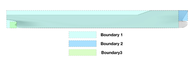
Fig. 3. Area division depends on different fixed directions. |
Table 5. Location of different areas and their fixed directions. |
| Boundary area | Area location | Fixed coordinate |
|---|---|---|
| Boundary-1 | x∈[−0.236,7.063] y∈[−0.572,0.063] z∈[−0.400,0.455] | X |
| Boundary-2 | x∈[−0.236,0.266] y∈[−0.572,0.063] z∈[−0.400,−0.105] | X,Z |
| Boundary-3 | x∈[7.0625,7.588] y∈[−0.572,0.063] z∈[−0.012,0.455] | X,Z |
Similar to the principal dimension modification parameters, the amount of the movement of the control points determines the geometry modification space of the hull form. Different areas of the ship have different degrees of influence on the ship hull performance, where the geometry modification of the bow and stern has a more significant impact on the performance of the ship, and the midship has a relatively low influence on the performance of the ship. To reflect the degree of influence for different hull areas, we set up different control point movement ranges according to different areas, making sure we can reduce the difficulty of training the DL model while ensuring sufficient geometry modification space. Fig. 4 shows the area division depends on the movement range of the control points, and Table 6 shows the location of different areas and the movement range of the control points in the area.

Fig. 4. Area division depends on the movement range of the control points. |
Table 6. Location of different areas and the movement range of the control points in the area. |
| Area | Location | Direction | Scope |
|---|---|---|---|
| SABED | x∈[7.063,7.588] y∈[−0.572,0.063] z∈[−0.400,−0.012] | X | [−0.1,0.1] |
| SACQM | x∈[−0.236,7.588] y∈[−0.572,0.063] z∈[−0.400,0.455] | Y | [−0.1,0.1] |
| SABPM | x∈[−0.236,7.588] y∈[−0.572,0.063] z∈[−0.400,−0.012] | Y | [−0.2,0.2] |
| SKLQP | x∈[−0.236,0.266] y∈[−0.572,0.063] z∈[−0.105,0.455] | Y | [−0.3,0.3] |
| SABHG | x∈[6.477,7.588] y∈[−0.572,0.063] z∈[−0.400,−0.012] | Y | [−0.3,0.3] |
| SABED | x∈[7.063,7.588] y∈[−0.572,0.063] z∈[−0.400,−0.012] | Y | [−0.4,0.4] |
| SKLQP | x∈[−0.236,0.266] y∈[−0.572,0.063] z∈[−0.105,0.455] | Z | [−0.2,0.2] |
| SABHG | x∈[6.477,7.588] y∈[−0.572,0.063] z∈[−0.400,−0.012] | Z | [−0.2,0.2] |
| SABED | x∈[7.0625,7.58811] y∈[−0.572,0.063] z∈[−0.400,−0.012] | Z | [−0.3,0.3] |
Based on the preset design space and the aforementioned measures to prevent unreasonable hull models, we can obtain as many hull model samples as possible to train the DL model. Benefitting from our setting for the movement range of the control points according to different hull areas, the randomly generated hull samples will continue to maintain a long parallel mid-body, and the middle part is basically flat instead of a lot of bumps and depressions. Moreover, due to the large movement range of the control points near the bow and stern, we can make drastic geometry modifications to the bow and stern. Fig. 5 shows a comparison between a randomly deformed hull model and the initial hull model, where we can notice the drastic geometry modifications at the bow area and a relatively minor modification at the mid-body.
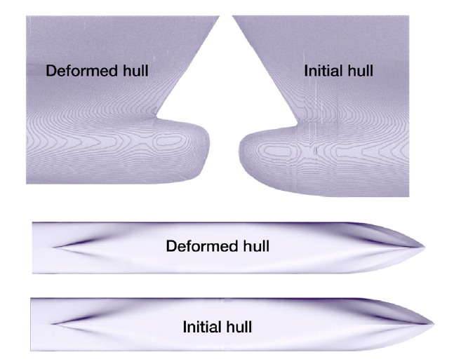
Fig. 5. Comparison of deformed hull model and initial hull model. |
3.4. Data collection
Training a DL model requires a dataset contains with large enough samples. In order to save the data collection process, we randomly generate geometric modification parameters according to the preset variable range to generate each hull model in the dataset. For the principal dimension modification parameters, we used continuous uniform distributions to generate them to make sure all samples can evenly distribute in the principal dimension design space. Besides, we used the truncated normal distribution [28], which is a normal distribution with upper and lower limits in sample space, to generate the movement amount of control points. The truncated normal distribution makes the movement amount of control points concentrated near the mean value, ensuring the hull form after geometry modification will be more likely similar to the initial KCS hull. Besides, since the more similar the hull form is to the initial hull form, the easier it is for the hull form to meet engineering requirements, and using a truncated normal distribution also means the hull form after geometry modification is more likely in line with engineering requirements.
The degree of similarity between the hull form after geometry modification and the initial hull form can be adjusted by changing the parameters in the truncated normal distribution. In detail, the smaller the standard deviation of the truncated normal distribution, the larger possibility the hull form keeps similar to the initial hull form. The larger the standard deviation of the truncated normal distribution, the greater the possibility of significant geometry modification. Eq. (19) provides the probability density function f(x) of the truncated normal distribution, which is determined by the mean μ, the standard deviation σ, low boundary value a, the upper boundary value b, and the probability density function ϕ and the cumulative distribution function Φ of the standard normal distribution,
Using continuous uniform distributions and truncated normal distributions to generate hull model samples can significantly reduce the time required for the data collection process. Meanwhile, not like manually generating hull model samples, randomly generating samples can make sure all samples can be as much as possible evenly distributed in the entire design space and also avoid the subjective influence of designers.
Before and after calculating the performance of hull samples, we checked the hull samples in the dataset twice to ensure the validity of the samples. Specifically, before calculating the performance of hull samples, we checked the hull forms in the dataset to ensure there are no unreasonable hull forms. After calculating the performance of hull samples, we checked the results and the wave pattern of all hull samples and eliminated all incorrect hull samples. The performance evaluation process of the dataset was conducted on a personal laptop computer (Alienware Area-51 m, CPU: Intel Core I9-9900 K, 3.60 GHz, RAM: 32.0 GB, and GPU: Nvidia Geforce RTX 2070). After performing evaluation and sample validity tests, we generated a dataset that contains 31,058 hull samples inside it.
4. Construction and training of the deep learning model
4.1. Fully connected neural network (FCNN)
DL technology has a unique ability to extract internal relationships from complex or even inaccurate data, thereby finding a mathematical model that is too complex for the human brain or other computer technologies [8]. In recent years, DL technology has developed rapidly and has been found to have many successful applications in many other fields not limited to computer science [29].
As one of the most representative DL methods, Fully Connected Neural Network (FCNN), also known as Artificial Neural Network (ANN), is a DL technology-based parallel computational machine learning method, whose feature is that neurons will receive the processed information from all neurons in the previous layer. Fig. 6 shows a schematic diagram of the topology structure of FCNN and a single neuron processing unit.
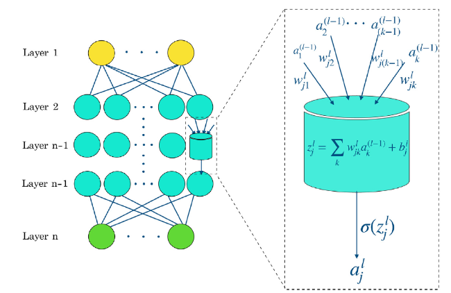
Fig. 6. The schematic diagram of FCNN topology structure and single neuron processing. |
Different layers perform different information transformation purposes in the FCNN model. Specifically, the input layer responsible for receiving data information from the outside world, which does not contain any calculation work. The hidden layer is equivalent to the information processing system, which is responsible for the main calculation work. Relying on the hidden layer, an FCNN model can extract internal rules from the dataset and store “memory” and “experience” in it. The most distinguishing feature of the FCNN model is that every hidden layer is fully connected with two adjacent layers, where each neuron in the layer l receives all neuron processed information in the layer (l−1) and then distributes its processed information to all neuron located in the layer (l+1). The output layer located at the end of the FCNN model is responsible for exporting predicted results to the outside world.
In this work, the input layer accepts the geometry modification parameters used to describe different hull forms, where each neuron in this layer represents an individual geometry modification parameter from a given sample in the dataset. The output layer, which coalesces the influence caused by the replacement of geometry modification parameters, exports the current inputted hull form performances. Due to the structure topology characteristics, when the FCNN model faces a large number of input parameters, it will become computationally intensive and prone to overfitting, leading to poor performance in specific tasks. However, many practices have proved that the FCNN model has shown stable performance in dealing with non-image-related tasks. Hence, considering that we need to build a model to simulate the function between the geometry modification parameters and the total resistance, which does not involve image processing, we choose the FCNN model as the DL model used in this work. Besides, unlike classification tasks, it is a better choice to keep the information channels of all neurons connected to uncover the actual mapping relationship of regression tasks. Therefore, we choose the FCNN model as the DL model used in this paper.
4.2. FCNN model construction
The DL model adopted in this paper is the FCNN model. A simplified schematic illustration of FCNN model is shown in Fig. 7. The input layer of the DL model contains 501 neurons, including length change rate, width change rate, height change rate, draught change rate, Froude number change rate, and the movement amount of all control points. It is worth noting that the order of all input neurons must be the same, and when we want to verify and use the DL model, we must also ensure that the order of input neurons does not change. The output layer of the DL model contains one neuron, which exports the total resistance of the current hull model.
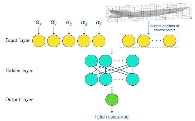
Fig. 7. Simplified schematic of the FCNN model. |
Before tuning the FCNN model, we need to set several hyperparameters to make the FCNN model ready to be tuned, including activation function, loss function, and the method to judge the prediction accuracy. The activation function is a mathematical converter that can transform the information of the current neuron into the information flowing into the next neuron. The purpose of setting the activation function is to add nonlinear properties to the DL model. To make the DL model easy to train without the vanishing gradient problem, the neurons in the input layer and hidden layer adopt the ReLU activation function [30], which is defined as the positive part of its argument,
Compared with the sigmoid function, ReLU is not easy to capture the performance of vanishing gradient, in which even when the activation function input reaches the boundary, the gradient of the neuron will not be too small. We adopted a linear activation function for neurons located in the output layer to ensure prediction accuracy, which is given as follow,
The loss function is an indicator for evaluating the completion degree of DL model training, where the lower the value of the loss function, the higher the training completion of the DL model. The loss function plays the role of supervisor and guides the update of weights and biases. This paper adopted the Mean Absolute Percentage Error (MAPE) [31], which is given as follow to direct the DL model to update to reduce the gap between the predicted result and the actual result,
where:
·N - total number of samples in dataset,
· - ith predicted value,
· - ith actual value.
The loss function value is an evaluation index that is easy for computers to understand since the only point that the machine needs to pay attention to reduce the value of the loss function as much as possible. However, when comparing the prediction accuracy between DL models, the value of the loss function becomes incomparable considering the different regularization parameters and different hidden structures. In this paper, we choose the mean and standard deviation of the absolute percentage difference of samples in the testing dataset as the indicators to determine the prediction accuracy between different DL models to avoid the influence caused by the different loss functions, which is shown as follows,
where:
· - total number of samples in the testing dataset,
· - ith absolute percentage error,
·μ - population means.
Note that represents the average of the absolute percentage differences of all samples in the testing dataset, representing the average prediction accuracy of the DL model. The smaller of a DL model, the higher the prediction accuracy the DL model is. is the standard deviation of the absolute percentage difference of all samples in the testing dataset, representing the degree of normalization of a DL model when predicting different hull forms. The smaller of the DL model, the higher the degree of normalization of a DL model.
The construction, training, and testing of the DL models were all developed based on the Keras framework [32] with the TensorFlow backend [33]. In the developed python code of the computer program, the (keras.models.Model) was adopted to construct the FCNN model, with (keras.layers.core.Dense) to add the hidden layer. The regularization parameters were added into the DL model by adopting (keras.regularizers.l1_l2) and (keras.layers.core.Dropout). The optimizer was established based on (keras.optimizers.Adam), with the access to adjust the initial learning rate and decay rate. All the tuning, training, and testing processes were conducted on a personal laptop computer with the following specifications: Alienware Area-51 m, CPU: Intel Core I9-9900 K, 3.60 GHz, RAM: 32.0 GB, and GPU: Nvidia Geforce RTX 2070.
4.3. Hyperparameters tuning
The tuning process is one of the most time-consuming stages in developing a deep learning method because almost all the hyperparameters are independent, and various hyperparameter combinations need to be tested to obtain the best or optimum combination. In the hyperparameters tuning process for the DL model used in this work, we need to determine hyperparameters including hidden layer structure, regularization parameters, dropout rate, learning rate, batch size, and training epochs.
For a supervised learning problem, it usually needs to divide the dataset into two parts: training dataset and testing dataset. In this research, we take 75% of samples in the dataset as the training dataset while using the remaining 25% of samples in the dataset as the testing dataset. In the actual computation, the total 31,058 hull structure samples were divided randomly into the ratios 23,293:7765.
The hidden layer structure determines the ultimate prediction capability of the DL model. Considering that we have selected FCNN as the DL model, we only need to determine the number of hidden layers and neurons in each hidden layer. We adopted L1, L2 regularization methods and the dropout technique to avoid overfitting, in which we add a correction term to the loss function as shown in Eq. (25),
where:
· - revised loss function,
· - L1 regularization rate,
· - L2 regularization rate,
· - jth parameter in the DL model.
There are other techniques that one may use to avoid overfitting, such as inactivating neurons randomly.
The learning rate controls the learning speed of the DL model, where the lower the learning rate, the slower the learning speed of the DL model. We can regard the training process of the DL model as to find extreme values in the n-dimensional parameter space (n is the number of the DL model parameters), and the learning rate determines the step size of the finding process. Considering the DL model is far away from the extreme point at the beginning of the training process, then an appropriately large learning rate can help shorten the epoch number required to approach the extreme value. Once the DL model is close to the extreme value, a lower learning rate is assigned to the DL model, which ensures that the DL model can continuously get close to the extreme value instead of oscillating near the extreme value. This process is described by the following equation,
where:
·i - the current epoch number,
· - the actual learning rate of ith epoch,
· - the initial learning rate,
· - the decay rate,
· - the total number of training epoch.
Here, we adopt a variable learning rate strategy that has the advantage to achieve large learning rate at the early stage while attain a small learning rate at the late stage, as shown in Eq. (26), where the current learning rate is related to the initial learning rate, and the learning decay rate is determined by the epoch number. As shown in Eq. (27) the learning decay rate will decrease with the increase of the epoch number.
Note that the number of epochs is a hyperparameter that defines the number of times that a learning algorithm will work through the entire training dataset. One epoch means that each sample in the training dataset has had an opportunity to update the internal model parameters.
An epoch has one or more batches, and the batch size is the number of samples fed in the DL model in each epoch. The purpose of the application of batch size is to reduce the memory required during training. Batch size is the amount of training data that the computer needs to process simultaneously, making the lower the batch size, the less memory required during the training process. Nevertheless, too small a batch size may result in inaccurate gradient values, leading to possible oscillations during training. Training epochs represent the total epoch number of the dataset through the DL model during the training process. In this research, the batch size was fixed to 4,096, considering the sample number in the training dataset. The training epochs are always the larger, the better, and we should set the training epochs as high as possible and decide whether to stop based on the loss function value.
In the hyperparameter tuning process, the most straightforward method is to try all hyperparameter combinations to select the best one. However, if we try all the possible combinations in actual operation, then we need to try tens of thousands of combinations, which is unacceptable in workload. Thus, we used some techniques to reduce the number of attempts required when doing the hyperparameters tuning process. In the beginning, we first keep all hyperparameters unchanged except the hidden layer structure and change the hidden layer structure of the DL model to obtain the most suitable hidden structure for predicting the total resistance of hull models, where the default hyperparameters are shown in Table 7.
Table 7. Default hyperparameters at the beginning of the tuning process. |
| Hyperparameters | Default value |
|---|---|
| L1 regularition rate | 0 |
| L2 regularition rate | 0 |
| Dropout rate | 0 |
| Batch size | 4096 |
We first determined the range of hidden layers number and the range of neurons number after comparing the capability and training time. We first set the number of hidden layers between 1 and 3. We also stipulate that the neurons in each layer are between 2 and 501 and must be a power of two. Simultaneously, considering that the number of input parameters is greater than the number of output parameters, we stipulate that the number of neurons in the back layer will not larger than the number of neurons in the front layer. We can obtain all the hidden layer structure possibilities through the above regulations and obtain the optimal hidden layer structure by training all DL models and comparing the indicators.
In this research, we adopted a rate finding method developed by Leslie Smith in [34] to automatically find the range of optimal learning rates, where the whole process of the rate finding method was explained in detail in Smith [34]. Based on the rate finding method, we create a loss vs. learning rate curve to show how the learning rate affects the value of the loss function, shown in Fig. 8. As shown in Fig. 8, we can visualize how the learning rate affects the training speed of the DL model, where the DL model loss value stays stable unless the learning rate exponentially increased from 10−10 to 10−8, which means when the learning rate is too low cause the DL model can not learn anything. When the learning rate arrived at 10−8, the learning rate is just large enough that our model can start learning, and when the learning rate arrived at 10−3, the DL model has a considerable learning speed. When the learning rate locates between 10−3 and 10−2, the learning speed of the DL model has a tiny change, expressed the increase of learning rate here can not improve too much training speed. By the time when the learning rate reaches 10−1, the loss value of the DL model begins to increase, meaning the learning rate is far too large. Based on the curve, we choose 5E−4 as the learning rate and choose 2000 as the training epoch number used for hyperparameters tuning, which gives the DL model a fast learning speed. Depending on the hidden layer structure, every step costs 9 and 10 us. We calculated 164 possible hidden layer structures, and Table 8 shows parts of tuning results with different hidden structures.

Fig. 8. Loss vs. learning rate curve. |
Table 8. Parts of tuning result of hidden structure. |
| Hidden sturcture | % (%) | % (%) |
|---|---|---|
| (64) | 24.898 | 24.131 |
| (256, 4) | 15.386 | 12.712 |
| (32, 32) | 13.473 | 12.071 |
| (128, 4, 2) | 9.882 | 8.357 |
Fig. 9 (a)-(d) show the training history of the four DL models mentioned in Table 8. As can be seen from these four images, we can find that the testing loss begins to increase, especially at epoch 2,000, compared with the decrease of the testing loss, meaning the DL model has overfitted, which can be avoided by tuning suitable regularization parameters.

Fig. 9. (a) Training history for (64), (b) Training history for (256, 4), (c) Training history for (32, 32), and (d) Training history for (128, 4, 2). |
We choose the hidden layer structure with relatively low and , no obvious overfitting, and low training loss as the final choice, which is (256,4,2). Then we used a hidden layer structure (256,4,2) to do further tuning to determine the regularization parameters, which can help us avoid overfitting and further train the DL model. Before tuning the regularization parameters, we set the range of all regularization parameters between 0 and 0.128. We calculated 729 possible regularization parameter combinations, and Table 9 shows parts of tuning results with different regularization parameters. Fig. 10(a)-(d) shows the training history of the four DL models mentioned in Table 9.
Table 9. Parts of tuning result of regularization parameters. |
| Empty Cell | L1 rate | L2 rate | dropout rate | % (%) | % (%) |
|---|---|---|---|---|---|
| case 1 | 0 | 0 | 0 | 26.167 | 194.706 |
| case 2 | 0.004 | 0.001 | 0.001 | 8.314 | 6.985 |
| case 3 | 0 | 0.128 | 0 | 6.512 | 5.752 |
| case 4 | 0.016 | 0 | 0.002 | 5.389 | 5.182 |

Fig. 10. (a) Training history for case 1, (b) Training history for case 2, (c) Training history for case 3, and (d) Training history for case 4. |
As shown in Fig. 10(a)-(d), the regularization parameters play an important role in preventing overfitting. By comparing the indicators and and ensure that overfitting does not occur, we finally set the L1 regularization parameter as 0.032, set the L2 regularization parameter as 0, and set the dropout rate as 0.
Finally, after tuning hidden structure and regularization parameters, all the hyperparameters of the final DL model are determined, which is shown in Table 10.
Table 10. Hyperparameters of the DL model at the beginning of the training process. |
| Hyperparameters | Value |
|---|---|
| Hidden sturcture | (256,4,2) |
| L1 regularition rate | 0.032 |
| L2 regularition rate | 0 |
| Dropout rate | 0 |
| Batch size | 4096 |
4.4. Training and testing
In this research, during the training process of the DL model, we used the technique of stopping and resuming the training process so that we can monitor the loss and reduce the loss by reducing the learning rate when needed. The entire training history of the DL model is shown in Fig. 11. Considering the training process lasted for 20,000 epoch, we divide it into two parts for better observation, showing the application of stopping and resuming technique.
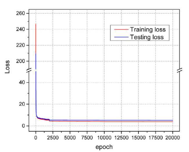
Fig. 11. The entire training history of the DL model. |
Fig. 12 (a) shows the training history of the DL model from epoch 0 to epoch 3000, where we set the initial learning rate as 10−3 and decrease the learning rate from 10−3 to 10−4 at epoch 2000. As shown in Fig. 12(a), both the training loss and the testing loss drop very quickly at the beginning, where the loss value decreases about %98% in the first 100 epoch compare with the whole training history, which means a relatively large learning rate can accelerate the initial training process. During epoch 100 to epoch 2000, both the training loss and the testing loss appear stochastic shock, but the overall trend is still declining, showing the DL model can still learn based on the current learning rate. The learning rate was decreased to 10−4 at epoch 2000, followed by a significant drop-down for both the training loss and the testing loss after epoch 2000.

Fig. 12. (a) The training history from epoch 1 to epoch 3,000, and (b) The training history from epoch 3000 to epoch 20,000. |
Fig. 12 (b) shows the training history of the DL model from epoch 3000 to epoch 20,000, where we decrease the learning rate from 10−4 to 10−5 at epoch 10,000. As shown in Fig. 12(b), the learning rate continued to decrease to 10−5 at epoch 10,000, followed by a relatively significant drop-down for both the training loss and the testing loss after epoch 16,000. Although it is not apparent, it can be noticed that the testing loss has risen slightly between epoch 10,000 to epoch 20,000, which means the appearance of overfitting. The DL model has been continued trained till it reached epoch 20,000, where there has no pronounced decrease for both the training loss and the testing loss.
We choose to stop the training process at epoch 19,900, where the testing loss reached the minimum in the entire training history, and we also store the DL model located at epoch 19.900 for further use. As shown in Table 11, the final training and testing loss values were close to each other. The shows that the average difference between the predicted and actual total resistance in the testing dataset is 3.9754%. The shows that the standard deviation between the predicted and actual total resistance in the testing dataset is 4.7562%. The results show that the DL model defined and trained in this work performs well in predicting the testing data, and no severe overfitting problem exists. The final trained DL model can be used to predict the total resistance of the hull form, which can evaluate the total resistance of the hull form modified from the KCS to assist the hull design stage.
Table 11. Training results of the final DL model. |
| Empty Cell | Loss | ||
|---|---|---|---|
| Training | 3.8844 | - | - |
| Testing | 5.1630 | 3.9754% | 4.7562% |
5. Model verification
The weights and biases of the deep learning model can be saved to be further used to predict the total resistance of the hull structure form generated by the geometric modification of the KCS. The most convenient of the DL model is that once we import all geometry modification parameters to the DL model, then the DL model can immediately evaluate the performance of the hull form, which can save the modeling and calculating workload, and designers do not need to consider any hydrodynamic theory. In real situations of engineering design of the hull form, the hull form after geometry modification will be randomly located in the design space, and it is most likely on the interval or gap space among training samples. However, the total resistances of hull forms located in the interval space are not contained in the training dataset, and they are very different from training samples. Predicting a case not located in the range of training samples is always a challenge, especially for the DL model in this paper, which needs to deal with the design space with 501 dimensions. To test the generality of the trained DL model, we performed several validation cases by comparing the result evaluated through the potential flow method and the DL model, in which the hull form after geometry modification is located in the interval space between training samples.
Considering that the geometry modification parameters contain the principal dimension modification parameters and the movement amount of control points, we verify the prediction accuracy of the DL model in three steps in different ways. In the first step, we verify the prediction accuracy of the DL model by fixing the movement amount of control points and when only the principal dimension modification parameters can be changed. To test the generality of the DL model, in step 1, we performed all testing cases when all the movement amount of control points equal to 0.05, ensuring the test cases do not have a chance to appear in the dataset. The details of the testing cases in step 1 are shown in Table 12. To be statistically representative, we also check the case in which the principal dimension is out of the domain by extending the range scope of principal dimensions.
Table 12. The details of the testing cases in step 1. |
| Testing case | Length rate | Breadth rate | Height rate | Draft rate | Froude number rate |
|---|---|---|---|---|---|
| Case 1 | (0.7, 1.3) | 1 | 1 | 0 | 1 |
| Case 2 | 1 | (0.7, 1.3) | 1 | 0 | 1 |
| Case 3 | 1 | 1 | (0.7, 1.3) | 0 | 1 |
| Case 4 | 1 | 1 | 1 | (−0.45, 0.05) | 1 |
| Case 5 | 1 | 1 | 1 | 0 | (0.6, 1.4) |
Fig. 13 (a) shows the curves for total resistance predicted by the potential flow method and the DL model when the length change rate in the scope range (0.7, 1.3) but the scope range of the dataset is (0.8, 1.2). For the entire range, the maximum error is 27.85%, located at 0.7, with the average error of all sample points in the entire range equals 6.90%. Moreover, for the domain, the maximum error is 7.90%, located at 0.85, with the average error of all sample points in the domain is 4.08% which can meet the engineering requirements of the hull form design stage.

Fig. 13. (a) Curve of total resistance vs. length change rate, and (b) Curve of total resistance vs. breadth change rate. |
Fig. 13 (b) shows the curves for total resistance predicted by the potential flow method and the DL model when the breadth change rate in the scope range (0.7, 1.3) but the scope range of the dataset is (0.8, 1.2). For the entire range, the maximum error is 13.93%, located at 1.3, with the average error of all sample points in the entire range equals 5.44%. Moreover, for the domain, the maximum error is 10.85%, located at 1.2, with the average error of all sample points in the domain is 4.92%.
Fig. 14 (a) shows the curves for total resistance predicted by the potential flow method and the DL model when the height change rate in the scope range (0.7, 1.3) but the scope range of the dataset is (0.8, 1.2). For the entire range, the maximum error is 15.64%, located at 1.3, with the average error of all sample points in the entire range equals 4.92%. Moreover, for the domain, the maximum error is 6.95%, located at 1.2, with the average error of all sample points in the domain is 4.25%.
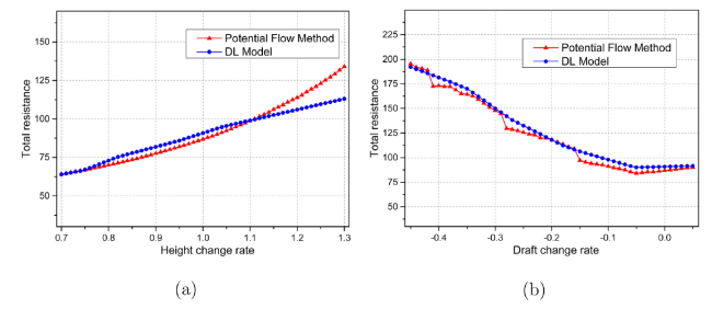
Fig. 14. (a) Curve of total resistance vs. height change rate, and (b) Curve of total resistance vs. draft change rate. |
Fig. 14 (b) shows the curves for total resistance predicted by the potential flow method and the DL model when the draft change rate in the scope range (−0.45, 0.05) but the scope range of the dataset is (−0.4, 0). For the entire range, the maximum error is 9.62%, located at −0.28, with the average error of all sample points in the entire range equals 4.22%. Moreover, for the domain, the maximum error is also 9.62%, located at −0.28, with the average error of all sample points in the domain is 4.63%.
Fig. 15 shows the curves for total resistance predicted by the potential flow method and the DL model when the Froude number change rate in the scope range (0.6, 1.4) but the scope range of the dataset is (0.7, 1.3). For the entire range, the maximum error is 33.87%, located at 0.6, with the average error of all sample points in the entire range equals 8.35%. Moreover, for the domain, the maximum error is 19.12%, located at 1.2, with the average error of all sample points in the domain is 5.67%.

Fig. 15. Curve of total resistance vs. Froude number change rate. |
In step 2, we performed all testing cases for different movement amounts of control points to test the generality of the DL model, ensuring the test cases do not have a chance to appear in the dataset. Considering that there are 406 parameters related to control points among the geometric modification parameters, it will be complicated to choose the movement amount of control points one by one. Hence, to test the generality of the DL model, we generated testing cases using linear functions to generate the movement amount of control points, avoiding the testing cases have a chance to appear in the training dataset. Assuming the movement amount of the first control point parameter is , and the movement amount of the last control point parameter is , then the movement amount of the ith control point parameter is given in the following equation,
Fig. 16 shows the curves for total resistance predicted by the potential flow method and the DL model when was in the scope range (−0.1, 0.1) and the was fixed to 0.1. The details of Case 6 in step 2 are shown in Table 13. Since the minimum scope range of the movement amount of control points is (−0.1, 0.1), all samples tested in step 2 are in the design space. For the entire range, the maximum error is 12.50%, located at −0.1, with the average error of all sample points is 3.09% which can meet the engineering requirements of the hull form design stage.
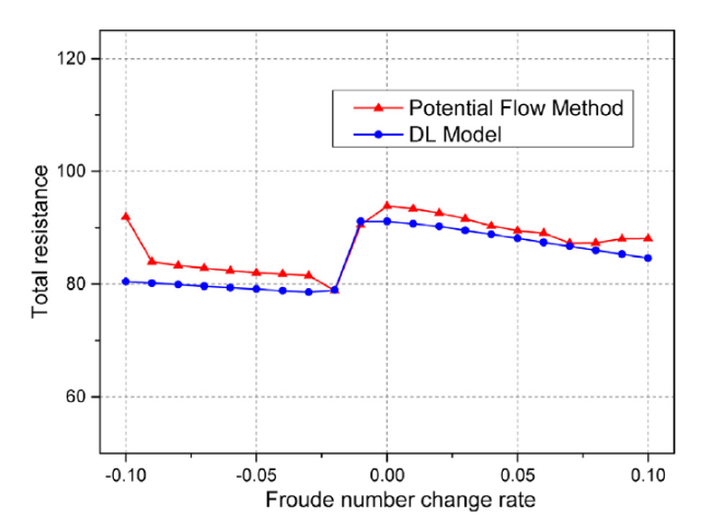
Fig. 16. Curve of total resistance of step 2. |
Table 13. The details of the testing cases in step 2. |
| Testing case | Length | Breadth | Height | Draft | Froude | ||
|---|---|---|---|---|---|---|---|
| Case 6 | 1 | 1 | 1 | 0 | 1 | (−0.1, 0.1) | 0.1 |
| Case 7 | 1 | 1 | 1 | 0 | (0.7, 1.3) | 0.1 | −0.07 |
| Case 9 | 1 | 1 | 1 | 0 | (0.7, 1.3) | −0.07 | 0.1 |
In step 3, we verify the prediction accuracy of the DL model by simultaneity change both the principal dimension parameters and the movement amount of control points to ensure the consistency for different kinds of geometry modification parameters. The details of Case 7 and Case 8 in step 3 are shown in Table 13. Fig. 17(a) shows the curves for total resistance predicted by the potential flow method and the DL model when was fixed to 0.1 and the was fixed to −0.07, with the Froude number change rate in the scope range (0.7, 1.3). For the domain range, the maximum error is 14.37%, located at 0.7, with the average error of all sample points in the domain range equals 4.68%.

Fig. 17. (a) Curve of total resistance of Case 6, and (b) Curve of total resistance of Case 7. |
Fig. 17 (b) shows the curves for total resistance predicted by the potential flow method and the DL model when was fixed to −0.07 and the was fixed to 0.1, with the Froude number change rate in the scope range (0.7, 1.3). For the domain range, the maximum error is 15.70%, located at 0.7, with the average error of all sample points in the domain range equals 4.48%.
The predicted errors of all testing cases in method verification are shown in Table 14. As shown in Table 14, the DL model can predict the total resistance of the hull form model generated by the geometry modification of the KCS with high prediction accuracy. It is worth noting that all cases tested in this chapter have never appeared in the dataset, meaning that the DL model we constructed and trained here can predict a sample it is never seen, which gives designers an excellent method to assist the hull design stage. We can find that the maximum error and average error in the entire range are almost always larger than the maximum error and average error in the domain range through the above test cases. Meanwhile, the maximum error in the domain range always happened in the boundary of the domain range, which shows that the prediction accuracy is related to the sample number in the training dataset and the distribution density of the samples in the design space, and the higher sample density, the higher prediction accuracy.
Table 14. Predicted errors in method verification. |
| Testing case | Max (entire) | Ave (entire) | Max (domain) | Ave (domain) |
|---|---|---|---|---|
| Case 1 | 27.85% | 6.90% | 7.90% | 4.08% |
| Case 2 | 13.93% | 5.44% | 10.85% | 4.92% |
| Case 3 | 15.64% | 4.92% | 6.95% | 4.25% |
| Case 4 | 9.62% | 4.22% | 9.62% | 4.63% |
| Case 5 | 33.87% | 8.35% | 19.12% | 5.67% |
| Case 6 | 12.50% | 3.09% | 12.50% | 3.09% |
| Case 7 | 14.37% | 4.68% | 14.37% | 4.68% |
| Case 8 | 15.70% | 4.48% | 15.70% | 4.48% |
6. Conclusions
In this work, we have developed a deep learning neural network model to predict the total resistance of ship hull form generated based on the geometry modification of the KRISO Container Ship (KCS), which can assist the hull form design at the preliminary ship design stage.
Expressly, we set the KRISO Container Ship (KCS) as the initial hull model and simplified the geometry modification process into a set of geometry modification parameters by combining the linear transformation method and Free-Form Deformation (FFD) technique. By randomly generating hull form samples and adopting a potential flow method to calculate the total resistance of all samples, we established a dataset used to train and test the DL model. The generality test shows that the trained DL model can predict the total resistance of hull forms accurately and quickly in the design stage, which is a remarkable success for applying deep learning techniques in the hull form design process. Based on this study, we have concluded that by using deep learning techniques, one can predict the performances of the hull form with high accuracy to meet the engineering requirements of the initial design.
The DL-based hull form performance prediction model developed in this work adopts the potential flow method generated data sample as the virtual training data to train a DL model and then uses it to predict actual hull performance. Considering that the initial design stage belongs to the preliminary design, which has a lower accuracy requirement than those in other design phases, the potential flow method adopted in this work has sufficient accuracy to meet the design requirements and has a faster speed of constructing the sample dataset. Furthermore, we think that the successful application of deep learning technology in this work offers an efficient method to assist the ship design process, with currently commonly used design methods incurring large time requirements due to the massive calculation workload of ship design.
In this work, we only take the total resistance as the only predictive target. The dataset only contains the hull form generated based on the geometry modification of the KCS, which means the final DL model can only predict the total resistance of specific hull forms. We can further expand the application range of the deep learning model by adding more hull models to the dataset, and we can also increase the prediction accuracy of the deep learning model by increasing the sample density. In work in progress, we may extend the prediction method to other performance of hull forms and further increase the design space by increasing the variety and number of dataset samples.
Declaration of Competing Interest
The authors declare that they have no known competing financial interestsor personal relationships that could have appeared to influence the work reported in this paper.
Acknowledgments
The work was performed in the University of California, Berkeley. YA is supported by a fellowship from China Scholar Council (No. 201806680134), and this support is greatly appreciated.
