
1. Introduction
The generalized theory of thermoelasticity has been the subject of intense research activities recently due to its widespread applications. The hyperbolic heat conduction equation of generalized theory emulates the experimentally observed finite speed of thermal signals and is known for its reliable predictions in many cases of interest. The initial successful attempts to formulate a generalized theory by modifying the classical coupled thermoelasticity theory which results in instantaneous thermal signals, are attributed to Lord-Shulman [1] and Green-Lindsay [2]. In Lord-Shulman model, the Fourier’s law is modified by including a thermal relaxation time parameter. On the other hand, two relaxation time parameters are used to formulate Green-Lindsay model. The constitutive relations were further modified by Green and Naghdi in their three additional models [3], [4], [5], which are used frequently to investigate the modeling of heat flow in various problems of thermoelasticity. Tzou [6] and Chandrasekharaiah [7] put forward the dual-phase-lag model of thermoelasticity. Further, Roychoudhuri [8] proposed three-phase-lag (TPL) thermoelastic model in which a phase-lag for the thermal displacement gradient is also included along with the phase-lags for the heat flux and the temperature gradient. Impacts of three-phase-lag on two-dimensional interactions in an isotropic medium with a spherical cavity were investigated by Banik and Kanoria [9]. Using TPL model, Shaw and Mukhopadhyay [10] investigated the surface wave propagation in an isotropic thermoelastic half-space having micropolarity effect. Kalkal et al. [11] considered the impacts of rotational field, ramp parameter and three-phase-lag in a thermo-viscoelastic medium with micropolarity. Sheokand et al. [12] analyzed the reflection phenomena of a fiber-reinforced orthotropic thermoelastic medium with a rotational effect. This investigation was carried out using three-phase-lag theory. Abo-Dahab et al. [13] used TPL model to analyze the impacts of temperature dependent properties and initial pressure on the plane wave propagation.
The porous materials have numerous applications in material science, geophysics, mechanics of bones, petroleum industry, drugs, medical devices industry, chemical engineering etc. In a double porosity model, we can use a macro and micro porosity structure simultaneously where the macro-porosity is due to the pores present in the body while the microporosity is due to the fissures in the considered body. The double porosity modeling of rocks and clay materials emulates the realistic geotechnical problems in a better way and has been the focus of recent research (Salimzadeh and Khalili [14]). Wilson and Aifantis [15] proposed a model for deformable materials having double porous structure. Iesan and Quintanilla [16] proposed a non-linear theory of thermoelasticity containing double porous structure. Kumar and Vohra [17] used Laplace transform method to study the response of a thermoelastic microbeam having double porous structure and laser pulse heating. Abdou et al. [18] analyzed a two dimensional problem of thermoelasticity having double porosity using L-S theory. In another article, Abdou et al. [19] measured the impact of Lorentz force on the thermo-mechanical interactions under Lord-Shulman theory having double porous feature.
The influence of the gravitational force in the classical theory of elasticity is generally ignored although it is important in many realistic situations. In context with L-S and DPL models, Abo-Dahab et al. [20] visualized the impacts of gravity and rotation parameter on an electro-magneto thermoelastic half-space having diffusivity and single porosity. Hilal et al. [21] considered the influences of micropolarity and gravity in a rotational medium having microtemperatures. Othman et al. [22] solved the problem of micropolar thermoelastic medium under the consideration of Green-Naghdi theory (with and without energy disippation) and gravitational field effect. The influences of Lorentz and gravitational force were discussed by Abd-Alla et al. [23] for magneto-thermoelastic medium using GN-II model. Recently, Laplace and Fourier transforms technique is employed by Othman et al. [24] to measure the impact of inclined load on a thermoelastic medium with gravitational field. The two dimensional equations are formulated under dual-phase-lag theory.
The functionally graded materials have non homogeneous composition where a gradual change of material composition with a corresponding variation of properties and the volume fraction of various composites takes place. On sudden cooling or heating of these materials, higher magnitude of thermal stresses are generated resulting in high temperature thermal shock. The excellent thermo-physical properties of FGMs make them the material of choice for pressure vessels, nuclear reactor structures and various components of industrial and chemical plants. Lotfy and Tantawi [25] discussed the photothermal elastic waves interactions in a non homogeneous medium including magnetic effect. By imposing an inclined load, the dynamical interactions in a non homogeneous, magneto-thermoelastic medium with micropolarity are studied by Kalkal et al. [26]. Recently, Gunghas et al. [27] investigated the two dimensional thermo-dynamical interactions in a non-homogeneous material having porosity and gravitational fields.
In the present work, we have analyzed two dimensional thermo-mechanical interactions in an isotropic, functionally graded half-space with double porosity under gravitational field effect under three-phase-lag model. A thermal load of constant intensity is exerted on the bounding surface. Normal mode methodology is adopted to obtain the appropriate results of the physical quantities. Simulation is done in a copper material using MATLAB software and results for various physical fields have been depicted graphically to show the effects of different parameters such as non homogeneity, gravity, double porosity and three-phase-lag.
After doing an extensive survey of literature, we have noticed that no thermoelastic problem comprising of non homogeneous thermoelastic half-space by including gravitational and double porosity parameters with three-phase-lag effect has been reported till now. The current research work is relevant for studying the problems related with thermal load, non-homogeneity parameter, gravity and double porosity. Thus, the thermoelastic investigation dealing with the inclusion of these parameters provides a more realistic model and its application can not be ruled out in the physical world.
2. Governing equations
In view of Iesan and Quintanilla [16], the basic equations for a half-space having double porous structure including gravitational field as a body force are:
Kinematic relation
Constitutive equations
$\zeta=-d e_{k k}-l \phi-p \psi+c \theta$
where λ and μ are Lame’s constants, , where is linear thermal expansion coefficient, are the constitutive coefficients, are stress components, is the displacement vector, and are denoting equilibrated stresses related to pores and fissures respectively, ϕ and ψ are volume fraction fields related to pores and fissures respectively, ξ and ζ are the intrinsic equilibrated body forces, is the cubical dilatation, T is absolute temperature, is the reference temperature of the medium in its natural state and is the Kronecker delta.
Stress equation of motion
$\sigma_{j i, j}+G_{i}=\rho \ddot{u}_{i}$
where is the gravitational force.
Equilibrated stress equations of motion
$\tau_{i, i}+\zeta=k_{2} \ddot{\psi}$
where and are the equilibrated inertia coefficients.
By using Eqs. (3)-(6) in (8) and (9), following equations are obtained
$\bar{b} \phi,{ }_{, i i}+\gamma \psi,{ }_{, i i}-d u_{r, r}-l \phi-p \psi+c \theta=k_{2} \ddot{\psi} .$
Equations of balance of energy
$\rho S=\beta e_{k k}+a \phi+c \psi+\frac{\rho C_{e} \theta}{T_{0}}$
where is the heat flux vector, S is the entropy per unit volume, ρ is the density and is the specific heat at constant strain.
Equation of heat conduction
$\left(1+\tau_{q} \frac{\partial}{\partial t}+\frac{\tau_{q}^{2}}{2} \frac{\partial^{2}}{\partial t^{2}}\right) q_{i}=K^{*}\left(1+\tau_{v} \frac{\partial}{\partial t}\right) v_{, i}+K\left(1+\tau_{T} \frac{\partial}{\partial t}\right) \theta_{, i}$
where is a material characteristic of the theory, K is the thermal conductivity and , , are the thermal relaxation times.
Using Eqs. (12)-(14), One can find the heat conduction equation for TPL model (Roychoudhuri [8]) as:
$\begin{array}{r} {\left[K^{*}\left(1+\tau_{v} \frac{\partial}{\partial t}\right)+K \frac{\partial}{\partial t}\left(1+\tau_{T} \frac{\partial}{\partial t}\right)\right] \nabla^{2} \theta=\left(1+\tau_{q} \frac{\partial}{\partial t}+\frac{\tau_{q}^{2}}{2} \frac{\partial^{2}}{\partial t^{2}}\right) \times} \\ {\left[\beta T_{0} \ddot{e}+a T_{0} \ddot{\phi}+c T_{0} \ddot{\psi}+\rho C_{e} \ddot{\theta}\right]} \end{array}$
Since FGMs are non homogeneous materials, parameters and c are not constant but vary with space co-ordinate. Thus, we consider
[ , c]=[ K0*,β0,h0, , , where , and are taken as constants along with as a non dimensional function of . Thus for a functionally graded medium, field equations and constitutive relations become:
$\begin{array}{l} {\left[K_{0}^{*} f(\vec{x})\left(1+\tau_{v} \frac{\partial}{\partial t}\right) \theta,{ }_{i}\right], i+\left[K_{0} f(\vec{x}) \frac{\partial}{\partial t}\left(1+\tau_{T} \frac{\partial}{\partial t}\right) \theta, i\right], i=} \\ f(\vec{x})\left(1+\tau_{q} \frac{\partial}{\partial t}+\frac{\tau_{q}^{2}}{2} \frac{\partial^{2}}{\partial t^{2}}\right)\left[\beta_{0} T_{0} \ddot{e}+a_{0} T_{0} \ddot{\phi}+c_{0} T_{0} \ddot{\psi}+\rho_{0} C_{e} \ddot{\theta}\right] \end{array}$
3. Problem formulation
Consider an isotropic, functionally graded thermoelastic medium having double porosity and gravitational field under three-phase-lag model. The rectangular cartesian co-ordinates are employed with origin on the surface x=0 and we choose x co-ordinate in the vertically downward direction. Present analysis is restricted to a two dimensional problem in xy-plane (Fig. 1). Thus, the displacement components are defined as:
$u=u(x, y, t), \quad v=v(x, y, t), \quad w=0$
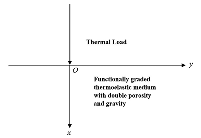
Fig. 1. The geometrical layout of the problem. |
It is also assumed that the material properties are graded along x-axis. Thus we take as . Considering expressions (21), the stresses obtained from (16) can be written as follows:
$\sigma_{x y}=\mu_{0} f(x)\left(\frac{\partial u}{\partial y}+\frac{\partial v}{\partial x}\right)$
The above equations can be simplified by using the following dimensionless quantities:
$\begin{array}{l} \begin{array}{l} \left(x^{\prime}, y^{\prime}\right)=\frac{\omega^{*}}{c_{1}}(x, y),\left(u^{\prime}, v^{\prime}\right)=\frac{\rho_{0} \omega^{*} c_{1}}{\beta_{0} T_{0}}(u, v),\left(t^{\prime}, \tau_{v}^{\prime}, \tau_{T}^{\prime}, \tau_{q}^{\prime}\right) \\ =\omega^{*}\left(t, \tau_{v}, \tau_{T}, \tau_{q}\right), \theta^{\prime}=\frac{\theta}{T_{0}} \\ \sigma_{i j}^{\prime}=\frac{\sigma_{i j}}{\beta_{0} T_{0}},\left(\phi^{\prime}, \psi^{\prime}\right)=\frac{k_{1_{0}} \omega^{* 2}}{m_{0}}(\phi, \psi),\left(\sigma_{1}^{\prime}, \tau_{1}^{\prime}\right) \\ =\frac{c_{1}}{\alpha_{0} \omega^{*}}\left(\sigma_{1}, \tau_{1}\right), g^{\prime}=\frac{g}{c_{1} \omega^{*}} \end{array}\\ \text { where }\\ \omega^{*}=\frac{\rho_{0} C_{e} c_{1}^{2}}{K_{0}}, c_{1}^{2}=\frac{\lambda_{0}+2 \mu_{0}}{\rho_{0}} \end{array}$
where
$\omega^{*}=\frac{\rho_{0} C_{e} c_{1}^{2}}{K_{0}}, c_{1}^{2}=\frac{\lambda_{0}+2 \mu_{0}}{\rho_{0}}$
g is the gravity field.
Now, we take , where n is a non homogeneity parameter and using the dimensionless quantities taken in (25), expressions (22)-(24) and (17)-(20) reduce to
$\sigma_{x y}=a_{4} e^{-n x}\left(\frac{\partial u}{\partial y}+\frac{\partial v}{\partial x}\right)$
$\begin{array}{l} {\left[\left(1+\tau_{v} \frac{\partial}{\partial t}\right)+a_{18} \frac{\partial}{\partial t}\left(1+\tau_{T} \frac{\partial}{\partial t}\right)\right]\left[\nabla^{2} \theta-n \frac{\partial \theta}{\partial x}\right]=} \\ \left(1+\tau_{q} \frac{\partial}{\partial t}+\frac{\tau_{q}^{2}}{2} \frac{\partial^{2}}{\partial t^{2}}\right) \times\left[a_{19} \frac{\partial^{2} e}{\partial t^{2}}+a_{20} \frac{\partial^{2} \phi}{\partial t^{2}}+a_{21} \frac{\partial^{2} \psi}{\partial t^{2}}+a_{22} \frac{\partial^{2} \theta}{\partial t^{2}}\right] \end{array}$
where
$\begin{array}{l} a_{1}=\frac{\lambda_{0}}{\rho_{0} c_{1}^{2}}, a_{2}=\frac{h_{0} m_{0}}{\beta_{0} k_{1_{0}} T_{0} \omega^{* 2}}, a_{3}=\frac{d_{0} m_{0}}{\beta_{0} k_{1_{0}} T_{0} \omega^{* 2}}, a_{4}=\frac{\mu_{0}}{\rho_{0} c_{1}^{2}}, a_{5}=a_{1}+a_{4} \\ a_{6}=\frac{\bar{b}_{0}}{\alpha_{0}}, a_{7}=\frac{h_{0} \beta_{0} T_{0} k_{1_{0}}}{\rho_{0} \alpha_{0} m_{0}}, a_{8}=\frac{m_{0} c_{1}^{2}}{\omega^{* 2} \alpha_{0}}, a_{9}=\frac{l_{0} c_{1}^{2}}{\omega^{* 2} \alpha_{0}}, a_{10}=\frac{a_{0} T_{0} k_{1_{0}} c_{1}^{2}}{\alpha_{0} m_{0}} \\ a_{11}=\frac{k_{1_{0}} c_{1}^{2}}{\alpha_{0}}, a_{12}=\frac{\gamma_{0}}{\bar{b}_{0}}, a_{13}=\frac{d_{0} \beta_{0} T_{0} k_{1_{0}}}{\rho_{0} \bar{b}_{0} m_{0}}, a_{14}=\frac{l_{0} c_{1}^{2}}{\omega^{* 2} \bar{b}_{0}}, a_{15}=\frac{p_{0} c_{1}^{2}}{\omega^{* 2} \bar{b}_{0}} \\ a_{16}=\frac{c_{0} T_{0} k_{1_{0}} c_{1}^{2}}{\bar{b}_{0} m_{0}}, a_{17}=\frac{k_{2_{0}} c_{1}^{2}}{\bar{b}_{0}}, a_{18}=\frac{\omega^{*} K_{0}}{K_{0}^{*}}, a_{19}=\frac{\beta_{0}^{2} T_{0}}{\rho_{0} K_{0}^{*}}, a_{20}=\frac{a_{0} c_{1}^{2} m_{0}}{k_{1_{0}} K_{0}^{*} \omega^{* 2}} \\ a_{21}=\frac{c_{0} c_{1}^{2} m_{0}}{k_{1_{0}} K_{0}^{*} \omega^{* 2}}, a_{22}=\frac{\rho_{0} C_{e} c_{1}^{2}}{K_{0}^{*}} \end{array}$
4. Solution of the problem
To solve the Eqs. (29)-(33), we employ normal mode technique and consider the solution as shown below:
$\begin{array}{l} \left(u, v, \phi, \psi, \theta, \sigma_{i j}, \sigma_{i}, \tau_{i}\right)(x, y, t)=\left(u^{*}, v^{*}, \phi^{*}, \psi^{*}, \theta^{*}, \sigma_{i j}^{*}\right. \\ \left.\sigma_{i}^{*}, \tau_{i}^{*}\right)(x) e^{(\omega t+l \kappa y)} \end{array}$
where and are the amplitudes of the physical quantities, ω is the complex frequency and κ is the wave number in y-direction. In view of expression (34), Eqs. (29)-(33) reduce to the following forms:
$a_{19} D u^{*}+b_{20} v^{*}+a_{20} \phi^{*}+a_{21} \psi^{*}-\left(\epsilon_{0} D^{2}-b_{21} D-b_{22}\right) \theta^{*}=0 \text {, }$
where
$\begin{array}{l} b_{0}=a_{4} \kappa^{2}+\omega^{2}, b_{1}=g+\iota a_{5} \kappa, b_{2}=\iota n \kappa a_{1}, b_{3} \\ =n a_{2}, b_{4}=n a_{3}, b_{5}=\iota \kappa a_{5}-g, \\ b_{6}=\iota n \kappa a_{4}, b_{7}=n a_{4}, b_{8}=\kappa^{2}+\omega^{2}, b_{9}=\iota \kappa a_{2}, b_{10} \\ =\iota \kappa a_{3}, b_{11}=\iota \kappa, b_{12}=\iota \kappa a_{7}, \\ b_{13}=\kappa^{2}+a_{8}+a_{11} \omega^{2}, b_{14}=n a_{6}, b_{15}=a_{6} \kappa^{2}+a_{9}, b_{16} \\ =\iota \kappa a_{13}, b_{17}=\kappa^{2}+a_{14}, \\ b_{18}=n a_{12}, b_{19}=a_{12} \kappa^{2}+a_{15}+a_{17} \omega^{2}, b_{20}=\iota \kappa a_{19}, \\ \epsilon_{0}=\left[\frac{\left(1+\tau_{v} \omega\right)+a_{18} \omega\left(1+\tau_{T} \omega\right)}{\omega^{2}\left(1+\tau_{q} \omega+\frac{\tau_{q}^{2}}{2} \omega^{2}\right)}\right], \\ b_{21}=n \epsilon_{0}, b_{22}=\epsilon_{0} \kappa^{2}+a_{22}. \end{array}$
The condition for existence of a non-trivial solution of the system of Eqs. (35)-(39) provides us the following tenth-order differential equation:
$\begin{array}{l} {\left[D^{10}+P_{1} D^{9}+P_{2} D^{8}+P_{3} D^{7}+P_{4} D^{6}+P_{5} D^{5}+P_{6} D^{4}+P_{7} D^{3}\right.} \\ \left.+P_{8} D^{2}+P_{9} D+P_{10}\right]\left(u^{*}, v^{*}, \phi^{*}, \psi^{*}, \theta^{*}\right)=0 \end{array}$
where are provided in “Appendix A”.
The solution of Eq. (40), which is bounded as x →∞ is given by
$\begin{array}{l} \begin{array}{r} \left(u^{*}, v^{*}, \phi^{*}, \psi^{*}, \theta^{*}\right)(x)=\sum_{i=1}^{5}\left(1, H_{1 i}, H_{2 i}, H_{3 i}, H_{4 i}\right) M_{i}(\kappa, \omega) e^{-\lambda_{i} x} \\ \text { for } \operatorname{Re}\left(\lambda_{i}\right)>0 \end{array}\\ \end{array}$
where are coefficients depending upon κ and ω. Inserting the solution (41) into the expressions for stresses (26)-(28), following relations are obtained:
$\left(\sigma_{x x}^{*}, \sigma_{x y}^{*}, \sigma_{y y}^{*}\right)(x)=\sum_{i=1}^{5}\left(H_{5 i}, H_{6 i}, H_{7 i}\right) M_{i}(\kappa, \omega) e^{-\lambda_{i} x-n x}$
In view of relations (25), (34) and (41), expressions for and (for non homogeneous system) can be obtained as:
$\left(\sigma_{x}^{*}, \tau_{x}^{*}\right)(x)=\sum_{i=1}^{5}\left(H_{8 i}, H_{9 i}\right) M_{i}(\kappa, \omega) e^{-\lambda_{i} x-n x}$
where all and are given in “Appendix B”.
5. Application
In this work, a functionally graded, isotropic, thermoelastic half-space having double porous structure and gravity with the half-space x≥0 is considered. To find the coefficients , we impose some boundary conditions along with a thermal load at the surface of half-space.
(1) Thermal boundary condition
The boundary plane x=0 is acted upon by a thermal load, hence, the thermal boundary condition is expressed as
$\theta(0, y, t)=\bar{h}(y, t)=h^{*} \exp (\omega t+\iota \kappa y)$
where function is dependent on y and t and is the magnitude of thermal load.
(2) Mechanical boundary conditions
The boundary plane x=0 is assumed to be stress free i.e.
$\sigma_{x x}(0, y, t)=0, \quad \sigma_{x y}(0, y, t)=0$
(3) Double porosity conditions
Double porosity conditions are vanishing of equilibrated stress corresponding to pores and fissures i.e.
$\sigma_{x}(0, y, t)=0, \quad \tau_{x}(0, y, t)=0$
Using expressions (41)-(43) and employing the method defined in (34), the boundary conditions lead to a non homogeneous system of five equations. These equations can be expressed as follows:
System (47) is solved by using Cramer’s rule to evaluate the coefficients i.e and expressions for the field variables such as displacement, stresses and temperature distribution for functionally graded material having double porosity and gravitational field are obtained as shown below
$\left(\sigma_{x x}^{*}, \sigma_{x y}^{*}, \sigma_{y y}^{*}, \sigma_{x}^{*}, \tau_{x}^{*}\right)(x)=\frac{1}{\Delta} \sum_{i=1}^{5}\left(H_{5 i}, H_{6 i}, H_{7 i}, H_{8 i}, H_{9 i}\right) \Delta_{i} e^{-\lambda_{i} x-n x}$
where Δ and are defined in “Appendix C”.
6. Special cases
6.1. Without double porosity
If we put into the field equations and constitutive relations, then the present problem reduces to a functionally graded medium having gravitational effect and expressions of various field variables are described as:
$\left(\sigma_{x x}^{*}, \sigma_{x y}^{*}, \sigma_{y y}^{*}\right)(x)=\frac{1}{\Delta^{*}} \sum_{i=1}^{3}\left(H_{3 i}^{\prime}, H_{4 i}^{\prime}, H_{5 i}^{\prime}\right) \Delta_{i}^{*} e^{-\lambda_{i} x-n x}$
where
$\begin{array}{l} \Delta^{*}=H_{21}^{\prime} L_{1}^{\prime}-H_{22}^{\prime} L_{2}^{\prime}+H_{23}^{\prime} L_{3}^{\prime}, \Delta_{1}^{*}=h^{*} L_{1}^{\prime}, \Delta_{2}^{*}=-h^{*} L_{2}^{\prime}, \Delta_{3}^{*}=h^{*} L_{3}^{\prime}, \\ L_{1}^{\prime}=\left(H_{32}^{\prime} H_{43}^{\prime}-H_{42}^{\prime} H_{33}^{\prime}\right), L_{2}^{\prime}=\left(H_{31}^{\prime} H_{43}^{\prime}-H_{41}^{\prime} H_{33}^{\prime}\right), L_{3}^{\prime}=\left(H_{31}^{\prime} H_{42}^{\prime}-H_{41}^{\prime} H_{32}^{\prime}\right), \\ H_{1 i}^{\prime}=\frac{J_{5} \lambda_{i}^{3}-J_{6} \lambda_{i}^{2}+J_{7} \lambda_{i}+J_{8}}{J_{0} \lambda_{i}^{4}-J_{1} \lambda_{i}^{3}+J_{2} \lambda_{i}^{2}+J_{3} \lambda_{i}+J_{4}}, H_{2 i}^{\prime}=\frac{-J_{9} \lambda_{i}^{3}+J_{10} \lambda_{i}^{2}-J_{11} \lambda_{i}-J_{12}}{J_{0} \lambda_{i}^{4}-J_{1} \lambda_{i}^{3}+J_{2} \lambda_{i}^{2}+J_{3} \lambda_{i}+J_{4}} \\ H_{3 i}^{\prime}=\left(-\lambda_{i}+\iota \kappa a_{1} H_{1 i}^{\prime}-H_{2 i}^{\prime}\right), H_{4 i}^{\prime}=a_{4}\left(\iota \kappa-\lambda_{i} H_{1 i}^{\prime}\right), H_{5 i}^{\prime} \\ =\left(-a_{1} \lambda_{i}+\iota \kappa H_{1 i}^{\prime}-H_{2 i}^{\prime}\right) \\ J_{0}=-a_{4} \epsilon_{0}, J_{1}=a_{4} b_{21}+b_{7} \epsilon_{0}, J_{2}=a_{4} b_{22}-b_{7} b_{21}+b_{8} \epsilon_{0}, J_{3}=b_{7} b_{22}+b_{8} b_{21} \\ J_{4}=b_{20} b_{11}-b_{8} b_{22}, J_{5}=-b_{5} \epsilon_{0}, J_{6}=b_{5} b_{21}+b_{6} \epsilon_{0}, J_{7}=b_{5} b_{22}-b_{6} b_{21}+a_{19} b_{11} \\ J_{8}=b_{6} b_{22}, J_{9}=-a_{19} a_{4}, J_{10}=a_{19} b_{7}, J_{11}=a_{19} b_{8}+b_{5} b_{20}, J_{12}=b_{6} b_{20}. \end{array}$
6.2. Without non homogeneity
By taking n=0 in Eqs. (29)-(33), we obtain expressions for various field variables from (48) and (49). In this limiting case, after neglecting the gravitational impact, we have compared our results with those of obtained by Abdou et al. [18] (by replacing L-S theory with three-phase-lag) with suitable modification in boundary and loading conditions.
6.3. Without gravity
The influence of gravitational field can be omitted from the medium by assuming g=0 in the equations of motion. It leads to a similar problem of functionally graded thermoelastic double porous medium. If we also eliminate the impact of non homogeneity in the considered case then our results agree with the results achieved by Abdou et al. [19] (after removing the magnetic field effect and replacing L-S theory with three-phase-lag) with suitable changes in boundary and loading conditions.
6.4. Without three-phase-lag
Three-phase-lag effect can be omitted from the medium by putting in the heat conduction equation. In this case if we take the parameters , then the expressions related to displacements, stresses and temperature field for a non homogeneous medium having single porous structure and gravitational field under GN-III theory can be obtained from expressions (48) and (49). Further, neglecting the impacts of non homogeneity parameter and gravity, our results are in good agreement with those reported by Abd-Elaziz and Hilal [28] (after removing electro-magnetic and Thomson impacts) with suitable changes in loading and boundary conditions.
7. Numerical results and discussion
$\begin{array}{l} \lambda_{0}=7.76 \times 10^{10} \mathrm{Nm}^{-2}, \mu_{0}=3.86 \times 10^{10} \mathrm{Nm}^{-2}, \alpha_{t}=1.78 \times 10^{-5} \mathrm{~K}^{-1}, \\ C_{e}=3.831 \times 10^{3} \mathrm{~m}^{2} \mathrm{~s}^{-2} \mathrm{~K}^{-1}, \rho_{0}=8954 \mathrm{~kg} \mathrm{~m}^{-3}, K_{0}=3.86 \times 10^{3} \mathrm{~N} \mathrm{~s}^{-1} \mathrm{~K}^{-1}, \\ T_{0}=293 \mathrm{~K}, \tau_{v}=0.1 \mathrm{~s}, \tau_{T}=0.2 \mathrm{~s}, \tau_{q}=0.3 \mathrm{~s}. \end{array}$
The values of double porosity parameters are taken from Khalili [30]:
$\begin{array}{l} \alpha_{0}=1.3 \times 10^{-5} \mathrm{~N}, m_{0}=2.3 \times 10^{10} \mathrm{Nm}^{-2}, p_{0}=2.4 \times 10^{10} \mathrm{Nm}^{-2}, \\ \gamma_{0}=1.1 \times 10^{-5} \mathrm{~N} \\ l_{0}=2.5 \times 10^{10} \mathrm{Nm}^{-2}, a_{0}=0.16 \times 10^{5} \mathrm{Nm}^{-2} \mathrm{~K}^{-1}, c_{0}=0.219 \times 10^{5} \mathrm{Nm}^{-2} \mathrm{~K}^{-1}, \\ \bar{b}_{0}=0.12 \times 10^{-5} \mathrm{~N}, d_{0}=0.1 \times 10^{10} \mathrm{Nm}^{-2}, k_{1_{0}}=0.1456 \times 10^{-12} \mathrm{Nm}^{-2} \mathrm{~s}^{2}, \\ k_{2_{0}}=0.1546 \times 10^{-12} \mathrm{Nm}^{-2} \mathrm{~s}^{2}, h_{0}=0.9 \times 10^{10} \mathrm{Nm}^{-2}. \end{array}$
Some other constants considered in the problem are taken as $\omega=2, \kappa=1.2, h^{*}=10$ In order to investigate the impacts of the considered parameters on different physical components, calculation and plotting is carried out using MATLAB software for the given data. Graphs are plotted for various values of x at t=0.01 and y=1.
Figs. 2 -6 depict the influence of non homogeneity parameter on the distribution of physical fields for three distinct values of n=0.000,n=0.001 and n=0.002. Fig. 2 illustrates the distribution of displacement component u versus x-axis for three distinct values of n as stated above. The displacement field values increase with increase in the value of n, which indicates that the non homogeneity parameter is enhancing the displacement component u. Fig. 3 is drawn to show the variations of normal stress with distance x for the distinct values of n as considered above. All the three curves corresponding to three distinct values of non homogeneity parameter are having a coincident starting point at x=0 as expected from the boundary condition. The presence of non homogeneity parameter has strong effect on the normal stress distribution quantitatively as well as qualitatively. The normal stress is compressive in the whole range for the homogeneous medium whereas it is tensile as well as compressive in the non homogeneous medium. Fig. 4 is drawn to predict the equilibrated stress behavior with distance x. The values are strongly influenced by non homogeneity parameter for x=0.4 onward, where the values of increase with non homogeneity parameter. The effect of parameter n on equilibrated stress with x-axis is illustrated in Fig. 5. The equilibrated stress shows a similar trend in all the three cases. As the magnitude of parameter n is increased, the numerical values of equilibrated stress increase and its impact fades far away from the boundary. The impact of parameter n is illustrated on temperature field through Fig. 6. The temperature variation curves predict almost similar trend for all the three cases. Numerical values of temperature increase slightly for higher values of n. The effect dies as one goes away from the boundary. The temperature field values are maximum at the boundary surface where thermal shock is applied. It decreases monotonically as distance x increases and reaches to steady-state near the thermal wave front.
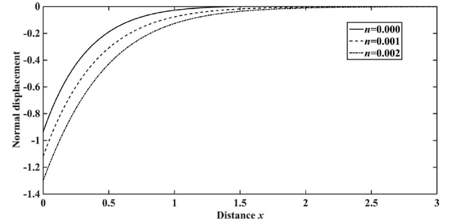
Fig. 2. Influence of FGM parameter on normal displacement. |
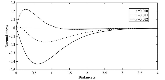
Fig. 3. Influence of FGM parameter on normal stress. |

Fig. 4. Influence of FGM parameter on equilibrated stress . |

Fig. 5. Influence of FGM parameter on equilibrated stress . |
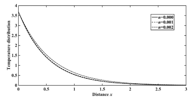
Fig. 6. Influence of FGM parameter on temperature field. |
Figs. 7 -11 are depicting the impact of phase-lag parameters on the variation of various physical quantities. Fig. 7 demonstrates that the value of the normal displacement for TPL model is slightly lower than that obtained using GN-III model. This predicts that phase-lag parameters have a diminishing impact on the profile of normal displacement. Fig. 8 displays the trend of normal stress curve with x-axis. The stress value starts from zero, increases with distance leading to a local maxima and then decreases to negative values attaining its maximum magnitude for x=0.9 and x=1.0 for TPL model and GN-III model respectively. Thereafter, it continuously diminishes to zero value for both of the models considered here. It can be also visualized that both curves follow similar trend. Fig. 9 represents the variations of equilibrated stress with distance for the TPL and GN-III models. Initially, the equilibrated stress values increase with distance leading to maximum value at about x=0.5, thereafter decrease continuously and approach to zero for both the models. The equilibrated stress values for GN-III model are slightly larger than three-phase-lag model for distance x=0.4 onwards. Fig. 10 depicts the behavior of equilibrated stress values with x-axis. We can visualize that the equilibrated stress for three-phase-lag theory has less numerical values as obtained from GN-III theory, which predicts the fact that phase-lag parameters are having a diminishing impact on the variation of equilibrated stress . Fig. 11 displays the temperature distribution with x-axis. It can be seen that the temperature field value for TPL theory is lower as compared to that obtained using GN-III theory although both of these models have same starting point. Hence, the phase-lag parameters behave as decreasing agents for the temperature field.
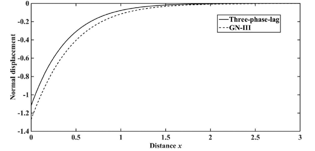
Fig. 7. Influence of phase-lags on normal displacement. |
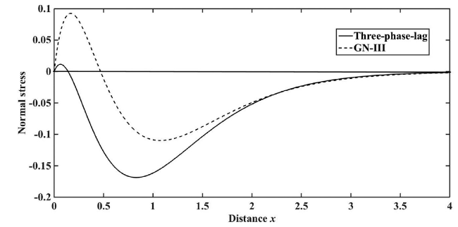
Fig. 8. Influence of phase-lags on normal stress. |
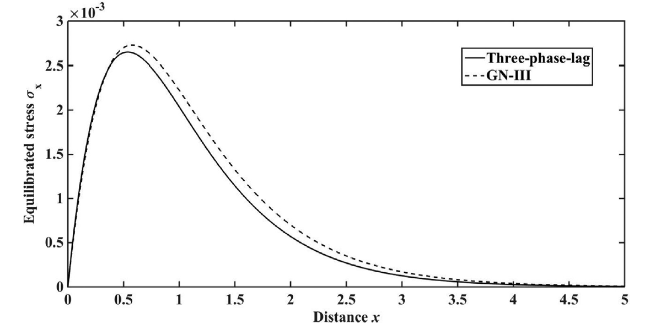
Fig. 9. Influence of phase-lags on equilibrated stress . |
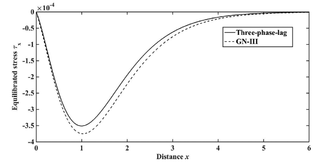
Fig. 10. Influence of phase-lags on equilibrated stress . |
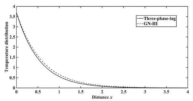
Fig. 11. Influence of phase-lags on temperature field. |
Figs. 12-16 are drawn to show the comparison of normal displacement, normal stress, equilibrated stresses and and temperature field for the three different media, namely, functionally graded thermoelastic medium with double porosity and gravity (FGMDPG), functionally graded thermoelastic medium with double porosity (FGMDP) and functionally graded thermoelastic medium with gravity (FGMG). In Fig. 12, we have shown the impacts of gravitational field and double porosity on the normal displacement versus x-axis. From the figure, it is clear that both double porosity and gravity parameters have a mixed impact on the magnitude of normal displacement. Fig. 13 shows the trend of normal stress values with x-axis. For FGMDPG and FGMG models, the magnitude and trends of normal stress curves are almost similar which indicates a small effect of double porosity on normal stress. On the other hand, switching off the gravity effect results in a significant increase in normal stress magnitude, showing a strong effect. By ignoring the gravitational effect, the value of normal stress curve peaks at x=0.5, thereafter it continuously decreases to zero. Figs. 14 and 15 illustrate the variations in equilibrated stresses and respectively for FGMDPG and FGMDP media. Higher numerical values of and are obtained for FGMDPG medium as compared to the FGMDP medium indicating that the inclusion of gravitational field enhances the modulus values of and . Fig. 16 depicts the temperature variation along x-axis for the three cases i.e. FGMDPG, FGMDP and FGMG. The temperature field values are maximum in the neighborhood of thermal source for all the three cases as expected from physical argument and thereafter damp to zero gradually. The boundary of the half-space is exposed to the thermal source leading to transmission of heat flux through infinitesimal elements of the half-space in sequence. In accordance with energy conservation law, a part of heat flux is used to increase the intrinsic energy of infinitesimal element resulting in increment of its temperature. The remaining part of the heat flux propagates further due to the presence of temperature gradient leading to heat conduction. It is also observed from the plot that the temperature values differ meagerly for all the three media, which indicates the little dependence of temperature on double porosity and gravitational field.

Fig. 12. Influence of double porosity and gravity on normal displacement. |
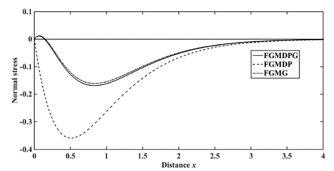
Fig. 13. Influence of double porosity and gravity on normal stress. |
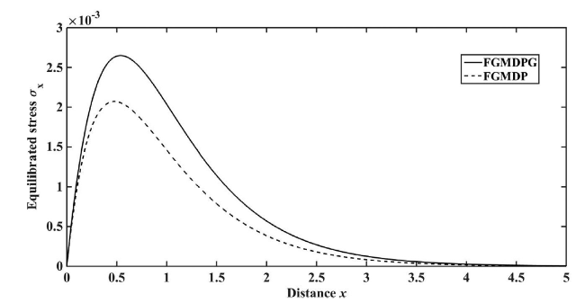
Fig. 14. Influence of gravity on equilibrated stress . |

Fig. 15. Influence of gravity on equilibrated stress . |

Fig. 16. Influence of double porosity and gravity on temperature field. |
8. Concluding remarks
Present work establishes a mathematical model for a functionally graded half-space having double porosity and gravitational field effects with TPL model. The obtained results reveal that the functionally graded parameter, gravitational field, double porosity and phase-lag parameters have significant impacts on all the considered fields. From this work, one can conclude that:
·The normal displacement, normal stress, equilibrated stresses and are significantly affected by non homogeneity parameter while a small effect is observed on temperature distribution. It enhances the value of normal displacement, equilibrated stress and temperature distribution while it diminishes as well as increases the normal and equilibrated stress values.
·The comparative study of three-phase-lag and GN-III theories suggest that the phase-lag parameters are significantly affecting the considered physical quantities. Phase-lag parameters exhibit damping impact on displacement component, equilibrated stress and temperature distribution whereas both increasing as well as decreasing effects are observed on normal stress and equilibrated stress in different regions.
·Double porosity effect is not very much significant on all the considered fields. Both increasing and decreasing impacts are observed on normal displacement while it slightly affects the magnitude of normal stress and temperature distribution.
·The gravitational field has a noticeable increasing effect on equilibrated stresses and while both increasing as well as decreasing effects are observed on normal displacement. It also diminishes the normal stress values.
·The methodology adopted here is widely used in many problems of thermodynamics and thermoelasticity.
The current research work can find its applications in seismology for understanding the earthquakes since present set of conditions are prevailing inside the earth. FGMs are widely used in the automobile industry, nuclear reactor, steel industry, medical field, defence industry and energy industry etc.
Declaration of Competing Interest
Authors declare that they have no conflict of interest.
Appendix A
$\begin{array}{l} C_{1}=-\epsilon_{0} a_{12}, C_{2}=a_{12} b_{21}+b_{18} \epsilon_{0}, C_{3}=a_{12} b_{22}-b_{18} b_{21}+b_{19} \epsilon_{0}, C_{4}=b_{22} b_{18} \\ +b_{19} b_{21} \\ C_{5}=b_{19} b_{22}+a_{21} a_{16}, C_{6}=b_{21}+n \epsilon_{0}, C_{7}=b_{22}-n b_{21}+\epsilon_{0} b_{17}, C_{8}=n b_{22}+b_{21} b_{17} \\ C_{9}=b_{22} b_{17}+a_{20} a_{16}, C_{10}=a_{21}-a_{12} a_{20}, C_{11}=a_{20} b_{18}-n a_{21}, C_{12}=a_{20} b_{19} \\ -b_{17} a_{21} \\ C_{13}=\epsilon_{0} b_{16}, C_{14}=b_{16} b_{21}, C_{15}=b_{16} b_{22}+b_{20} a_{16}, C_{16}=-a_{12} b_{20}, C_{17}=b_{18} b_{20} \\ C_{18}=b_{19} b_{20}-b_{16} a_{21}, C_{19}=b_{17} b_{20}-b_{16} a_{20}, C_{20}=a_{13} \epsilon_{0}, C_{21}=a_{13} b_{21} \\ C_{22}=a_{13} b_{22}+a_{16} a_{19}, C_{23}=-a_{19} a_{12}, C_{24}=a_{19} b_{18}, C_{25}=a_{19} b_{19}-a_{13} a_{21} \\ C_{26}=n a_{19}, C_{27}=b_{17} a_{19}-a_{13} a_{20}, C_{28}=a_{19} b_{16}-a_{13} b_{20}, C_{29}=C_{1}+a_{6} \epsilon_{0} \\ C_{30}=C_{2}-n C_{1}-a_{6} C_{6}-\epsilon_{0} b_{14}, C_{31}=C_{3}-n C_{2}-b_{13} C_{1}-a_{6} C_{7}+b_{14} C_{6}-\epsilon_{0} b_{15} \\ C_{32}=C_{4}+n C_{3}+b_{13} C_{2}-a_{6} C_{8}-b_{14} C_{7}-C_{6} b_{15} \\ C_{33}=n C_{4}-C_{5}-b_{13} C_{3}+a_{10} C_{10}+a_{6} C_{9}-b_{14} C_{8}+C_{7} b_{15}, \\ C_{34}=n C_{5}+b_{13} C_{4}+a_{10} C_{11}-b_{14} C_{9}-C_{8} b_{15}, \\ C_{35}=b_{13} C_{5}+a_{10} C_{12}-C_{9} b_{15}, C_{36}=-C_{1} b_{12}-a_{6} C_{13}, C_{37}=-C_{2} b_{12}+a_{6} C_{14} \\ +b_{14} C_{13} \\ C_{38}=a_{10} C_{16}-b_{12} C_{3}+a_{6} C_{15}-b_{14} C_{14}+b_{15} C_{13}, C_{39}=b_{12} C_{4}+a_{10} C_{17}-b_{14} C_{15} \\ -b_{15} C_{14}, \end{array}$
$\begin{array}{l} C_{40}=b_{12} C_{5}+a_{10} C_{18}-b_{15} C_{15}, C_{41}=b_{12} \epsilon_{0}-C_{13}, C_{42}=-b_{12} C_{6}+C_{14}+n C_{13}, \\ C_{43}=C_{15}-b_{12} C_{7}-a_{10} b_{20}-n C_{14}+b_{13} C_{13}, C_{44}=b_{12} C_{8}+n a_{10} b_{20}-n C_{15} \\ -b_{13} C_{14}, \\ C_{45}=b_{12} C_{9}+a_{10} C_{19}-b_{13} C_{15}, C_{46}=-C_{16}-a_{6} b_{20}, C_{47}=n C_{16}-C_{17}+n a_{6} b_{20} \\ +b_{14} b_{20}, \\ C_{48}=-b_{12} C_{10}-C_{18}+n C_{17}+b_{13} C_{16}+a_{6} C_{19}-n b_{14} b_{20}+b_{15} b_{20}, \\ C_{49}=n C_{18}-b_{12} C_{11}-b_{14} C_{19}+b_{13} C_{17}-n b_{15} b_{20}, C_{50}=b_{13} C_{18}-b_{12} C_{12}-b_{15} C_{19}, \\ C_{51}=-a_{7} C_{1}-a_{6} C_{20}, C_{52}=a_{6} C_{21}-a_{7} C_{2}+b_{14} C_{20}, \\ C_{53}=a_{10} C_{23}-a_{7} C_{3}+a_{6} C_{22}-b_{14} C_{21}+b_{15} C_{20}, \\ C_{54}=a_{7} C_{4}+a_{10} C_{24}-b_{14} C_{22}-b_{15} C_{21}, C_{55}=a_{7} C_{5}+a_{10} C_{25}-b_{15} C_{22}, C_{56}=a_{7} \epsilon_{0} \\ -C_{20}, \\ C_{57}=C_{21}-a_{7} C_{6}+n C_{20}, C_{58}=a_{7} C_{7}+a_{10} a_{19}-C_{22}+n C_{21}-b_{13} C_{20}, \\ C_{59}=a_{7} C_{8}+a_{10} C_{26}-n C_{22}-b_{13} C_{21}, C_{60}=a_{7} C_{9}+a_{10} C_{27}-b_{13} C_{22}, C_{61} \\ =-a_{6} a_{19}-C_{23}, \\ C_{62}=a_{6} C_{26}+b_{14} a_{19}-C_{24}+n C_{23}, C_{63}=a_{6} C_{27}-a_{7} C_{10}-b_{14} C_{26}+b_{15} a_{19}-C_{25} \\ +n C_{24}+b_{13} C_{23}, \\ C_{64}=b_{13} C_{24}+n C_{25}-b_{15} C_{26}-b_{14} C_{27}-a_{7} C_{11}, C_{65}=b_{13} C_{25}-b_{15} C_{27}-a_{7} C_{12}, \\ C_{66}=b_{12} C_{20}-a_{7} C_{13}, C_{67}=a_{7} C_{14}-b_{12} C_{21}, C_{68}=a_{7} C_{15}-b_{12} C_{22}+a_{10} C_{28}, \end{array}$
$\begin{array}{l} C_{69}=-a_{7} C_{16}+b_{12} C_{23}+a_{6} C_{28}, C_{70}=b_{12} C_{24}-a_{7} C_{17}-b_{14} C_{28} \\ C_{71}=-a_{7} C_{18}+b_{12} C_{25}-b_{15} C_{28}, C_{72}=a_{7} b_{20}+C_{28}-b_{12} a_{19}, C_{73}=b_{12} C_{26} \\ -n a_{7} b_{20}-n C_{28}, \\ C_{74}=b_{12} C_{27}-a_{7} C_{19}-b_{13} C_{28}, d_{1}=a_{4} C_{29}, d_{2}=a_{4} C_{30}-b_{7} C_{29}, d_{3}=a_{4} C_{31} \\ -b_{7} C_{30}-b_{8} C_{29} \\ d_{4}=-a_{4} C_{32}-b_{7} C_{31}-b_{8} C_{30}, d_{5}=a_{4} C_{33}+b_{7} C_{32}-b_{8} C_{31}-b_{9} C_{36} \\ +b_{10} C_{41}+b_{11} C_{46} \\ d_{6}=a_{4} C_{34}-b_{7} C_{33}+b_{8} C_{32}-b_{9} C_{37}+b_{10} C_{42}+b_{11} C_{47} \\ d_{7}=a_{4} C_{35}-b_{7} C_{34}-b_{8} C_{33}-b_{9} C_{38}+b_{10} C_{43}+b_{11} C_{48} \\ d_{8}=b_{11} C_{49}+b_{10} C_{44}-b_{9} C_{39}-b_{8} C_{34}-b_{7} C_{35}, d_{9}=b_{11} C_{50} \\ +b_{10} C_{45}-b_{9} C_{40}-b_{8} C_{35} \\ d_{10}=b_{5} C_{29}, d_{11}=b_{5} C_{30}-b_{6} C_{29}, d_{12}=b_{5} C_{31}-b_{6} C_{30} \\ -b_{9} C_{51}+b_{10} C_{56}+b_{11} C_{61}, \\ d_{13}=b_{11} C_{62}+b_{10} C_{57}-b_{9} C_{52}-b_{6} C_{31}-b_{5} C_{32}, d_{14}=b_{5} C_{33} \\ +b_{6} C_{32}-b_{9} C_{53}-b_{10} C_{58}+b_{11} C_{63}, \\ d_{15}=b_{5} C_{34}-b_{6} C_{33}-b_{9} C_{54}+b_{10} C_{59}+b_{11} C_{64}, d_{16}=b_{5} C_{35} \\ -b_{6} C_{34}-b_{9} C_{55}+b_{10} C_{60}+b_{11} C_{65} \\ d_{17}=b_{6} C_{35}, d_{18}=-a_{4} C_{51}, d_{19}=b_{7} C_{51}-a_{4} C_{52}, d_{20}=b_{5} C_{36} \\ -a_{4} C_{53}+b_{7} C_{52}+b_{8} C_{51} \end{array}$
$\begin{array}{l} d_{21}=b_{5} C_{37}-b_{6} C_{36}-a_{4} C_{54}+b_{7} C_{53}+b_{8} C_{52} \\ d_{22}=b_{5} C_{38}-b_{6} C_{37}+b_{10} C_{66}+b_{11} C_{69}-a_{4} C_{55}+b_{7} C_{54}+b_{8} C_{53} \\ d_{23}=b_{5} C_{39}-b_{6} C_{38}+b_{10} C_{67}+b_{11} C_{70}+b_{7} C_{55}+b_{8} C_{54} \\ d_{24}=b_{5} C_{40}-b_{6} C_{39}+b_{10} C_{68}+b_{11} C_{71}+b_{8} C_{55}, d_{25}=-b_{6} C_{40} \\ d_{26}=-a_{4} C_{56} \\ d_{27}=b_{7} C_{56}-a_{4} C_{57}, d_{28}=a_{5} C_{41}+a_{4} C_{58}+b_{7} C_{57}+b_{8} C_{56} \\ d_{29}=a_{5} C_{42}-b_{6} C_{41-} a_{4} C_{59}-b_{7} C_{58}+b_{8} C_{57} \\ d_{30}=b_{11} C_{72}+b_{9} C_{66}+b_{5} C_{43}-b_{6} C_{42}-a_{4} C_{60}+b_{7} C_{59}-b_{8} C_{58} \\ d_{31}=b_{9} C_{67}+b_{11} C_{73}+b_{5} C_{44}-b_{6} C_{43}+b_{7} C_{60}+b_{8} C_{59} \\ d_{32}=b_{9} C_{68}+b_{11} C_{74}+b_{5} C_{45}-b_{6} C_{44}+b_{8} C_{60}, d_{33}=b_{6} C_{45} \\ d_{34}=-a_{4} C_{61}, \\ d_{35}=b_{7} C_{61}-a_{4} C_{62}, d_{36}=b_{5} C_{46}-a_{4} C_{63}+b_{7} C_{62}+b_{8} C_{61} \\ d_{37}=b_{5} C_{47}-b_{6} C_{46}-a_{4} C_{64}+b_{7} C_{63}+b_{8} C_{62} \\ d_{38}=b_{9} C_{69}-b_{10} C_{72}+b_{5} C_{48}-b_{6} C_{47}-a_{4} C_{65}+b_{7} C_{64}+b_{8} C_{63} \\ d_{39}=b_{9} C_{70}-b_{10} C_{73}+b_{5} C_{49}-b_{6} C_{48}+b_{7} C_{65}+b_{8} C_{64} \\ d_{40}=b_{9} C_{71}-b_{10} C_{74}+b_{5} C_{50}-b_{6} C_{49}+b_{8} C_{65}, d_{41}=b_{6} C_{50} \\ P_{1}=\left(d_{2}-n d_{1}\right) / d_{1}, \\ P_{2}=\left(d_{3}-n d_{2}-b_{0} d_{1}-b_{1} d_{10}+a_{2} d_{18}-d_{34}-a_{3} d_{26}\right) / d_{1} \\ P_{3}=\left(d_{4}-n d_{3}-b_{0} d_{2}-b_{1} d_{11}+a_{2} d_{19}-b_{3} d_{18}+b_{2} d_{10}\right. \\ \left.+n d_{34}-d_{35}-a_{3} d_{27}+b_{4} d_{26}\right) / d_{1}, \end{array}$
$\begin{array}{l} P_{4}=\left(d_{5}-n d_{4}-b_{0} d_{3}-b_{1} d_{12}+a_{2} d_{20}-b_{3} d_{19}+b_{2} d_{11}\right. \\ \left.+n d_{35}-d_{36}-a_{3} d_{28}+b_{4} d_{27}\right) / d_{1}, \\ P_{5}=\left(d_{6}-n d_{5}-b_{0} d_{4}-b_{1} d_{13}+a_{2} d_{21}-b_{3} d_{20}+b_{2} d_{12}\right. \\ \left.+n d_{36}-d_{37}-a_{3} d_{29}+b_{4} d_{28}\right) / d_{1}, \\ P_{6}=\left(d_{7}-n d_{6}-b_{0} d_{5}-b_{1} d_{14}+a_{2} d_{22}-b_{3} d_{21}+b_{2} d_{13}\right. \\ \left.+n d_{37}-d_{38}-a_{3} d_{30}+b_{4} d_{29}\right) / d_{1}, \\ P_{7}=\left(d_{8}-n d_{7}-b_{0} d_{6}-b_{1} d_{15}+a_{2} d_{23}-b_{3} d_{22}+b_{2} d_{14}\right. \\ \left.+n d_{38}-d_{39}-a_{3} d_{31}+b_{4} d_{30}\right) / d_{1}, \\ P_{8}=\left(d_{9}-n d_{8}-b_{0} d_{7}-b_{1} d_{16}+a_{2} d_{24}-b_{3} d_{23}+b_{2} d_{15}\right. \\ \left.+n d_{39}-d_{40}-a_{3} d_{32}+b_{4} d_{31}\right) / d_{1}, \\ P_{9}=\left(-n d_{9}-b_{0} d_{8}+b_{1} d_{17}+a_{2} d_{25}-b_{3} d_{24}+b_{2} d_{16}\right. \\ \left.+n d_{40}+d_{41}+a_{3} d_{33}+b_{4} d_{32}\right) / d_{1}, \\ P_{10}=\left(-b_{0} d_{9}-b_{3} d_{25}-b_{2} d_{17}-n d_{41}-b_{4} d_{33}\right) / d_{1}. \end{array}$
Appendix B
$\begin{aligned} H_{0 i} & =d_{1} \lambda_{i}^{8}-d_{2} \lambda_{i}^{7}+d_{3} \lambda_{i}^{6}-d_{4} \lambda_{i}^{5}+d_{5} \lambda_{i}^{4}-d_{6} \lambda_{i}^{3}+d_{7} \lambda_{i}^{2}-d_{8} \lambda_{i}+d_{9}, \\ H_{1 i} & =\left(d_{10} \lambda_{i}^{7}-d_{11} \lambda_{i}^{6}+d_{12} \lambda_{i}^{5}-d_{13} \lambda_{i}^{4}+d_{14} \lambda_{i}^{3}-d_{15} \lambda_{i}^{2}+d_{16} \lambda_{i}+d_{17}\right) / H_{0 i} \\ H_{2 i} & =\left(-d_{18} \lambda_{i}^{7}+d_{19} \lambda_{i}^{6}-d_{20} \lambda_{i}^{5}+d_{21} \lambda_{i}^{4}-d_{22} \lambda_{i}^{3}+d_{23} \lambda_{i}^{2}-d_{24} \lambda_{i}+d_{25}\right) / H_{0 i} \\ H_{3 i} & =\left(d_{26} \lambda_{i}^{7}-d_{27} \lambda_{i}^{6}+d_{28} \lambda_{i}^{5}-d_{29} \lambda_{i}^{4}+d_{30} \lambda_{i}^{3}-d_{31} \lambda_{i}^{2}+d_{32} \lambda_{i}+d_{33}\right) / H_{0 i}, \\ H_{4 i} & =\left(-d_{34} \lambda_{i}^{7}+d_{35} \lambda_{i}^{6}-d_{36} \lambda_{i}^{5}+d_{37} \lambda_{i}^{4}-d_{38} \lambda_{i}^{3}+d_{39} \lambda_{i}^{2}-d_{40} \lambda_{i}-d_{41}\right) / H_{0 i}, \\ H_{5 i} & =\left(-\lambda_{i}+\iota \kappa a_{1} H_{1 i}+a_{2} H_{2 i}+a_{3} H_{3 i}-H_{4 i}\right), H_{6 i}=\left(\iota \kappa a_{4}-\lambda_{i} H_{1 i}\right), \\ H_{7 i} & =\left(-a_{1} \lambda_{i}+\iota \kappa H_{1 i}+a_{2} H_{2 i}+a_{3} H_{3 i}-H_{4 i}\right), H_{8 i}=-\left(\eta_{1} H_{2 i}+\eta_{2} H_{3 i}\right) \lambda_{i}, \\ H_{9 i} & =-\left(\eta_{2} H_{2 i}+\eta_{3} H_{3 i}\right) \lambda_{i}, \\ \eta_{1} & =\frac{m_{0}}{k_{10} \omega^{* 2}}, \eta_{2}=\frac{\bar{b}_{0} m_{0}}{k_{1_{0}} \omega^{* 2} \alpha_{0}}, \eta_{3}=\frac{\gamma_{0} m_{0}}{k_{1_{0}} \omega^{* 2} \alpha_{0}}. \end{aligned}$
Appendix C
$\begin{array}{l} \Delta=H_{41} L_{1}-H_{42} L_{2}+H_{43} L_{3}-H_{44} L_{4}+H_{45} L_{5}, \\ \Delta_{1}=h^{*} L_{1}, \quad \Delta_{2}=-h^{*} L_{2}, \Delta_{3}=h^{*} L_{3}, \Delta_{4}=-h^{*} L_{4}, \Delta_{5}=h^{*} L_{5}, \\ L_{1}=H_{52} d_{1}^{\prime}-H_{53} d_{2}^{\prime}+H_{54} d_{3}^{\prime}-H_{55} d_{4}^{\prime}, L_{2}=H_{51} d_{1}^{\prime}-H_{53} d_{5}^{\prime}+H_{54} d_{6}^{\prime}-H_{55} d_{7}^{\prime}, \\ L_{3}=H_{51} d_{2}^{\prime}-H_{52} d_{5}^{\prime}+H_{54} d_{8}^{\prime}-H_{55} d_{9}^{\prime}, L_{4}=H_{51} d_{3}^{\prime}-H_{52} d_{6}^{\prime}+H_{53} d_{8}^{\prime}-H_{55} d_{10}^{\prime}, \\ L_{5}=H_{51} d_{4}^{\prime}-H_{52} d_{7}^{\prime}+H_{53} d_{9}^{\prime}-H_{54} d_{10}^{\prime}, \\ d_{1}^{\prime}=H_{63} B_{1}-H_{64} B_{2}+H_{65} B_{3}, d_{2}^{\prime}=H_{62} B_{1}-H_{64} B_{4}+H_{65} B_{5}, \\ d_{3}^{\prime}=H_{62} B_{2}-H_{63} B_{4}+H_{65} B_{6}, d_{4}^{\prime}=H_{62} B_{3}-H_{63} B_{5}+H_{64} B_{6}, \\ d_{5}^{\prime}=H_{61} B_{1}-H_{64} B_{7}+H_{65} B_{8}, d_{6}^{\prime}=H_{61} B_{2}-H_{63} B_{7}+H_{65} B_{9}, \\ d_{7}^{\prime}=H_{61} B_{3}-H_{63} B_{8}+H_{64} B_{9}, d_{8}^{\prime}=H_{61} B_{4}-H_{62} B_{7}+H_{65} B_{10}, \\ d_{9}^{\prime}=H_{61} B_{5}-H_{62} B_{8}+H_{64} B_{10}, d_{10}^{\prime}=H_{61} B_{6}-H_{62} B_{9}+H_{63} B_{10}, \\ B_{1}=H_{84} H_{95}-H_{85} H_{94}, B_{2}=H_{83} H_{95}-H_{85} H_{93}, B_{3}=H_{83} H_{94}-H_{84} H_{93}, \\ B_{4}=H_{82} H_{95}-H_{92} H_{85}, B_{5}=H_{82} H_{94}-H_{92} H_{84}, B_{6}=H_{82} H_{93}-H_{83} H_{92}, \\ B_{7}=H_{81} H_{95}-H_{91} H_{85}, B_{8}=H_{81} H_{94}-H_{84} H_{91}, B_{9}=H_{81} H_{93}-H_{83} H_{91}, \\ B_{10}=H_{81} H_{92}-H_{82} H_{91}. \end{array}$
