
1. Introduction
Water waves are a prominent natural phenomenon. The analysis of water ripples and their various transformations is crucial to fluid dynamics in general and ocean phenomena in particular [1], [2], [3]. Water waves inspired the conception of nonlinear dispersive waves and solitons from a physics perspective. Numerous researchers, including Korteweg and de Vries, have addressed the KdV equation as a mathematical model for shallow water waves in streams and oceans, laying the foundations for the idea of solitary waves. Since then, the KdV-type equations have gained significance, with applications ranging from including internal gravity waves in lakes with various cross-sections, ion-acoustic waves in plasmas, and interfacial waves in a two-layer liquid with varying depths being identified [4], [5], [6]. As a result, numerous explored and developed approaches in nonlinear partial differential equations, such as symmetry groups, Bäcklund transformation, Painléve analysis, and the trail equation approach, are based on the KdV-type problem [7], [8], [9], [10]. Numerous researchers have devoted their interest to developing analytical and numerical approaches for obtaining various sorts of nonlinear PDEs; see [11], [12], [13], [14], [15].
The enormous variety and quality of evidence that must be incorporated into the modelling process in order for it to be as realistic as possible is a major challenge. The procedure of developing mathematical methods is subject to constraints, such as appropriate comprehension, uncertainty in precision and unpredictability, and mis-classification that contribute to parametric variations. Fuzzy simulation is a valuable tool for researchers to communicate technical difficulties. Several well-known areas have potential application of fuzzy set theory, such as control systems, knowledge-based systems, image processing, power engineering, industrial automation, robotics, consumer electronics, artificial intelligence/expert systems, management, and operations research.
Fractional calculus has been acknowledged as a highly valuable framework for addressing sustainability and complex phenomena for the past thirty years, due to its advantageous qualities such as nonlocality, heritability, high reliability, and analyticity [16], [17], [18]. The modified fractional notion was developed in order to address the challenges involved with processes, including inhomogeneities. Various innovators established the underlying framework, as well as their perspectives on expanding calculus, including Liouville, Hadamard, Caputo, Grunwald, Letnikov, Abel, Riez, Caputo-Fabrizio, Atangana-Baleanu (AB), researched the use of the fractional derivative and fractional differential equations (FDEs), see [19], [20]. Numerous essential interactions in electromagnetics, acoustics, viscoelasticity, electrochemistry, and material science are well explained by FDEs [21], [22].
Some researchers have broadened the definition of derivatives in the fuzzy setting in order to use fuzzy differential equations as a modelling framework for complex systems. This enables the formulation of differential equations in a fuzzy framework, as investigated by such authors [23].
When faced with actual occurrences, partial differential equations aren’t always the appropriate choice. We require to accumulate information from millions of domains in order to simulate complex behavior. These aspects of data sets are frequently ambiguous. Modeling complex systems with uncertain data has propelled fuzzy partial differential equations to the forefront of current mathematical modeling, capturing the attention of a slew of authors [24]. Fuzzy set theory has been widely applied in several domains, i.e., fixed-point theory, topology, fractional calculus, integral inequalities, image processing, bifurcation, control theory, consumer electronics, artificial intelligence, and operations research, [25], [26].
Chang and Zadeh [27] were the first to suggest the fuzzy derivative notion, which was quickly adopted by numerous other researchers [28]. Hukuhara’s publication [29] is the main focus of the concept of set valued DEs and fuzzy DEs. The Hukuhara derivative served as the foundation for the investigation of set DEs and, thereafter, fuzzy fractional DEs. Agarwal et al. in [30] reported the fuzzy Riemann-Liouville fractional differential equations leveraging the notion of Hukuhara differentiability, which was the basic foundation for the theme of fuzzy fractional derivatives. To handle ambiguous fractional differential equations, they adopted the Riemann-Liouville differentiability notion, relying on Hukuhara differentiability. The stability analysis of the solution for Riemann-Liouville fuzzy fractional DEs has been expounded in [31], [32]. Allahviranloo et al. [33] addressed explicit solutions to unpredictable fractional DEs under Riemann-Liouville -differentiability incorporating Mittag-Leffler mechanisms in [34], and formed fuzzy fractional DEs under Riemann-Liouville -differentiability incorporating fuzzy Laplace transforms. They demonstrated two novel existence theorems for fuzzy fractional differential equations using Riemann-Liouville generalized -differentiability and fuzzy Nagumo and Krasnoselskii-Krein criteria [35]. Arqub et al. [36] employed the reproducing kernel algorithm for the solution of two-point fuzzy boundary value problems. The fuzzy Fredholm-Volterra integrodifferential equations have been solved by the adaptation of the reproducing kernel algorithm by [37]. Ahmad et al. [38] studied the third order fuzzy dispersive PDEs in the Caputo, Caputo-Fabrizio, and Atangana-Baleanu fractional operator frameworks. Shah et al. [28] presented the evolution of one dimensional fuzzy fractional PDEs. To the best of our knowledge, the authors [39], [40] developed the novel extended approach and new numerical solutions for fuzzy conformable fractional differential equations and constructed the numerical solutions for fuzzy differential equations using the reproducing kernel Hilbert space method. Bushneq et al. [41] explored the ‘findings of fuzzy singular integral equations with an Abel’s type kernel using a novel hybrid method. In [42], Zia et al. adopted a semi-analytical technique for obtaining the solutions of fuzzy nonlinear integral equations. Salahshour et al. [43] expounded the -differentiability with Laplace transform to solve the FDEs.
When it comes to discovering solutions to significant challenges, researchers prefer integral transformations. The Laplace transformation was used on biological population, prey-predator and disease models in [44], [45]. Many researchers employed multiple integral transforms (Elzaki, Swai, Mohand, modified Laplace, Shehu, Aboodh) to develop exact solutions to important difficulties in dynamics, inorganic chemistry, and biological sciences, see [46], [47], [48].
Following this propensity, Jafari [49] contemplated the generalized integral transform (GIT) is a significant transformation in its entirety. A variant of the GIT is the, Laplace, ρ-Laplace, Elzaki, Aboodh, Natural, Swai, Sumudu, Kamal, Mohand, Pourreza, G-transform and Shehu transform, see [50], [51], [52], [53], [54], [55], [56], [57], [58], [59], [60], [61].
The focus of this research is to suggest a sophisticated homotopy perturbation transform method [62], [63] that can handle nonlinear partial fuzzy differential equations employing the fuzzy generalized integral transformation. Formulae are converted to algebraic expressions using the fuzzy general integral transform. The nonlinear components of the problem are then handled using the He’s polynomial [64], [65] approach to achieve the solution. The fuzzy generalized homotopy perturbation method is the name given to the novel perturbation method.
In this research, we propose a semi-analytical approach to the generalized homotopy perturbation transform method via fuzzy set theory. The aforesaid approach is used to construct the parametric form of the fuzzy mappings and is considered to be a valuable tool for solving the fuzzy dispersive and fifth order KdV models under fuzzy initial conditions. The generic model for the investigation of magneto-acoustic waves in plasma and shallow water waves with surface tension is the fifth order KdV equations. The integral transform applied here, in general, is the refinement of several existing transforms. Moreover, numeruous applications of the proposed algorithm are presented via the different fractional order and uncertainty parameter Also, their 2D and 3D simulations show the applicability of the method over the other methods. As a consequence, each finding generates a pair of solutions that are closely in agreement with the exact one. However, we have the choice to attain the appropriate one. Finally, as a part of our concluding remarks, we discussed the accumulated facts of our findings.
2. Fundamental ideas of fractional and fuzzy calculus
1. ∇ is normal (for some ),
2. ∇ is upper semi continuous,
3. i.e ∇ is convex;
4. is compact.
Definition 2.2. ([67]) We say that a fuzzy number ∇ is -level set described as
$[\nabla]^{\wp}=\{\Psi \in \mathbb{R}: \nabla(\Psi) \geq 1\}$
where and
Definition 2.3. ([67]) The parameterized version of a fuzzy number is denoted by such that satisfies the subsequent assumptions:
1. $\underset{}{\mathop{\nabla }}\,\left( \wp \right)$ is non-decreasing, left continuous, bounded over (0,1] and left continuous at 0.
2. is non-increasing, right continuous, bounded over (0,1] and right continuous at 0.
3.
Definition 2.4. ([68]) For and be a scalar. Assume that there are two fuzzy numbers then the addition, subtraction and scalar multiplication, respectively are stated as
1.
2.
3. $\Upsilon \odot \tilde{\gamma_{1}}=\left\{\left(\Upsilon \underline{\gamma_{1}}, \Upsilon \overline{\gamma_{1}}\right) \Upsilon \geq 0, \$ \Upsilon \overline{\gamma_{1}}, \Upsilon \underline{\gamma_{1}}\right) \Upsilon<0 .$
Definition 2.5. ([69]) Suppose a fuzzy mapping having two fuzzy numbers then Ψ-distance between and is represented as
$\Psi\left(\tilde{\gamma_{1}}, \tilde{\gamma_{2}}\right)=\sup _{\wp \in[0,1]}\left[\max \left\{\left|\underline{\gamma_{1}}(\wp)-\underline{\gamma_{2}}(\wp)\right|,\left|\overline{\gamma_{1}}(\wp)-\overline{\gamma_{2}}(\wp)\right|\right\}\right] .$
$\Psi\left(w(u), w\left(u_{0}\right)\right)<\epsilon ; \quad \text { whenever }\left|u-u_{0}\right|<\delta$
then is known to be continuous.
Definition 2.8. ([67]) Suppose that and Then is said to be strongly generalized differentiable at if exists such that (i)
(ii)
Throughout this investigation, we use the notation Ψ is (1)-differentiable and (2)-differentiable, respectively, if it is differentiable under the assumption (i) and (ii) defined in the above definition.
Theorem 2.1. ([68]) Consider a fuzzy valued function such that $ \Psi\left(\epsilon_{0} ; \wp\right)=\left[\Psi\left(\epsilon_{0} ; \wp\right), \bar{\Psi}\left(\epsilon_{0} ; \wp\right)\right] \text { and } \wp \in[0,1] \text {. }$Then
I. $\underline{\Psi}\left(\epsilon_{0} ; \wp\right)$ and are differentiable, if Ψ is a (1)-differentiable, and
$\left[\Psi^{\prime}\left(\epsilon_{0}\right)\right]^{\wp}=\left[\underline{\Psi^{\prime}}\left(\epsilon_{0} ; \wp\right), \bar{\Psi}^{\prime}\left(\epsilon_{0} ; \wp\right)\right]$
II. $\underline{\Psi}\left(\epsilon_{0} ; \wp\right)$ are differentiable, if Ψ is a (2)-differentiable, and
$\left[\Psi^{\prime}\left(\epsilon_{0}\right)\right]^{\wp}=\left[\bar{\Psi}^{\prime}\left(\epsilon_{0} ; \wp\right), \underline{\Psi^{\prime}}\left(\epsilon_{0} ; \wp\right)\right]$
Definition 2.9. ([69]) Assume that a fuzzy mapping ΨgH(r)=Ψ(r)∈CF[p]⋂LF[p]. Then, fuzzy -fractional Caputo differentiabilty of fuzzy-valued mapping Ψ is represented as
$\begin{array}{l} \left({ }_{g \mathcal{H}}^{c} \mathcal{D}^{\alpha} \Psi\right)(\omega)=\mathcal{J}_{a_{1}}^{r-\alpha} \odot\left(\Psi^{(r)}\right)(\epsilon) \\ =\frac{1}{\Gamma(r-\alpha)} \odot \int_{a_{1}}^{\omega}\left(\omega-\mathbf{W}_{2}\right)^{r-\alpha-1} \odot \Psi^{(r)}\left(\mathbf{w}_{2}\right) d \mathbf{w}_{2} \\ \alpha \in(r-1, r], \quad r \in \mathbb{N}, \omega>a_{1} \end{array}$
Therefore, the parameterized versions of and then CFD in fuzzy sense is stated as
$\left[\mathcal{D}_{(i)-g \mathcal{H}}^{\alpha} \Psi\left(\omega_{0}\right)\right]_{\wp}=\left[\mathcal{D}_{(i)-g \mathcal{H}}^{\alpha} \underline{\Psi}\left(\omega_{0}\right), \mathcal{D}_{(i)-g \mathcal{H}}^{\alpha} \bar{\Psi}\left(\omega_{0}\right)\right], \wp \in[0,1]$
where
$\begin{array}{l} {\left[\mathcal{D}_{(i)-g \mathcal{H}}^{\alpha} \underline{\Psi}\left(\omega_{0}\right)\right]} \\ =\frac{1}{\Gamma(r-\alpha)}\left[\int_{0}^{\omega}\left(\omega-\mathbf{w}_{2}\right)^{r-\alpha-1} \frac{d^{r}}{d \mathbf{w}_{2} r} \underline{\Psi}_{(i)-g \mathcal{H}}\left(\mathbf{w}_{2}\right) d \mathbf{w}_{2}\right] \omega=\omega_{0} \\ {\left[\mathcal{D}_{(i)-g \mathcal{H}}^{\alpha} \bar{\Psi}\left(\omega_{0}\right)\right]} \\ =\frac{1}{\Gamma(r-\alpha)}\left[\int_{0}^{\omega}\left(\omega-\mathbf{w}_{2}\right)^{r-\alpha-1} \frac{d^{r}}{d \mathbf{w}_{2}{ }^{r}} \bar{\Psi}_{(i)-g \mathcal{H}}\left(\mathbf{w}_{2}\right) d \mathbf{w}_{2}\right] \omega=\omega_{0} \end{array}$
Definition 2.10. Assume that a fuzzy mapping and α∈[0,1], then fuzzy -fractional Atangana-Baleanu differentiabilty of fuzzy-valued mapping is represented as
$\left(g \mathcal{H} \mathcal{D}^{\alpha} \Psi\right)(\omega)=\frac{\mathbb{B}(\alpha)}{1-\alpha} \odot\left[\int_{0}^{\omega} \underline{\Psi}^{\prime}\left(\mathbf{w}_{\mathbf{2}}\right) \odot E_{\alpha}\left[\frac{-\alpha\left(\omega-\mathbf{w}_{2}\right)^{\alpha}}{1-\alpha}\right] d \mathbf{w}_{2}\right]$
Thus, the parameterized formulation of and then the fuzzy Atangana-Baleanu derivative in Caputo sense is stated as
$\begin{array}{l} {\left[{ }^{A B C} \mathcal{D}_{(i)-g \mathcal{H}}^{\alpha} \tilde{\Psi}\left(\omega_{0} ; \wp\right)\right]} \\ =\left[{ }^{A B C} \mathcal{D}_{(i)-g \mathcal{H}}^{\alpha} \underline{\Psi}\left(\omega_{0} ; \wp\right),{ }^{A B C} \mathcal{D}_{(i)-g \mathcal{H}}^{\alpha} \bar{\Psi}\left(\omega_{0} ; \wp\right)\right], \wp \in[0,1] \end{array}$
where
$\begin{array}{l} { }^{A B C} \mathcal{D}_{(i)-g \mathcal{H}}^{\alpha} \underline{\Psi}\left(\omega_{0} ; \wp\right) \\ =\frac{\mathbb{B}(\alpha)}{1-\alpha}\left[\int_{0}^{\omega} \underline{\Psi}_{(i)-g \mathcal{H}}^{\prime}\left(\mathbf{w}_{2}\right) E_{\alpha}\left[\frac{-\alpha\left(\omega-\mathbf{w}_{2}\right)^{\alpha}}{1-\alpha}\right] d \mathbf{w}_{2}\right] \omega=\omega_{0} \\ { }^{A B C} \mathcal{D}_{(i)-g \mathcal{H}}^{\alpha} \bar{\Psi}\left(\omega_{0} ; \wp\right) \\ =\frac{\mathbb{B}(\alpha)}{1-\alpha}\left[\int_{0}^{\omega} \bar{\Psi}_{(i)-g \mathcal{H}}^{\prime}\left(\mathbf{w}_{2}\right) E_{\alpha}\left[\frac{-\alpha\left(\omega-\mathbf{w}_{2}\right)^{\alpha}}{1-\alpha}\right] d \mathbf{w}_{2}\right] \omega=\omega_{0} \end{array}$
where denotes the normalize function that equals to 1 when α assumed to be 0 and 1. Also, we suppose that type ype (𝑖)−𝑔𝐻 exists. exists. So here is no need to consider differentiability.
Recently, Jafari [49] defined the generalized integral transform. We extend this concept to fuzzy set theory.
Definition 2.11. Consider a continuous real-valued mappings such that Also, there be a continuous real-valued mapping and there is an improper fuzzy Riemann-integrable mapping on [0,∞). Then, the integral is known to be fuzzy generalized integral transform and is stated over the set of mappings:
$\mathcal{J}=\{\tilde{\Psi}(\omega): \exists \mathcal{A}, \kappa>0,|\tilde{\Psi}(\omega)|<\mathcal{A} \exp (\kappa \omega), \quad \text { if } \omega \geq 0\}$
As
$\begin{array}{l} \mathbb{J}[\tilde{\Psi}(\omega), \mathfrak{s}]=\mathbf{J}(\mathfrak{s}) \\ =\Theta(\mathfrak{s}) \int_{0}^{\infty} \exp (-\Phi(\mathfrak{s}) \omega) \odot \tilde{\Psi}(\omega) d \omega, \quad \Theta(\mathfrak{s}) \neq 0 \end{array}$
Remark 2.1. Definition 2.11 leads to the following conclusions:
1. Choosing and then we get the fuzzy Laplace transform.
2. Choosing and then we get the fuzzy α-Laplace transform.
3. Choosing and then we get the fuzzy Sumudu transform.
4. Choosing and then we get the fuzzy Aboodh transform.
5. Choosing and then we get the fuzzy Pourreza transform.
6. Choosing and then we get the fuzzy Elzaki transform.
7. Choosing and then we get fuzzy the Natural transform.
8. Choosing and then we get the fuzzy Mohand transform.
9. Choosing and then we get the fuzzy Swai transform.
10. Choosing and then we get the Kamal transform.
11. Choosing and then we get the fuzzy G−transform.
In (2.13), fulfilled the assumption of the decreasing diameter and increasing diameter of a fuzzy mapping Ψ.
Using the fact of Salahshour et al. [33], we have
$\begin{array}{l} \Theta(\mathfrak{s}) \int_{0}^{\infty} \exp (-\Phi(\mathfrak{s}) \omega) \odot \tilde{\Psi}(\omega) d \omega \\ =\left(\Theta(\mathfrak{s}) \int_{0}^{\infty} \exp (-\Phi(\mathfrak{s}) \omega) \underline{\Psi}(\omega) d \omega, \Theta(\mathfrak{s}) \int_{0}^{\infty} \exp \right. \\ (-\Phi(\mathfrak{s}) \omega) \bar{\Psi}(\omega) d \omega) \end{array}$
Also, considering the classical generalized integral transform proposed by Jafari [49], we get
$\mathbb{J}[\underline{\Psi}(\omega ; \wp)]=\Theta(\mathfrak{s}) \int_{0}^{\infty} \exp (-\Phi(\mathfrak{s}) \omega) \underline{\Psi}(\omega ; \wp) d \omega$
And
$\mathbb{J}[\underline{\Psi}(\omega ; \wp)]=\Theta(\mathfrak{s}) \int_{0}^{\infty} \exp (-\Phi(\mathfrak{s}) \omega) \underline{\Psi}(\omega ; \wp) d \omega$
Then, the aforesaid expressions can be written as
$\begin{aligned} \mathbb{J}[\tilde{\Psi}(\omega)] & =(\mathbb{J}[\underline{\Psi}(\omega ; \wp)], \mathbb{J}[\bar{\Psi}(\omega ; \wp)]) \\ & =(\underline{\mathcal{J}}(\mathfrak{s}), \overline{\mathcal{J}}(\mathfrak{s})) \end{aligned}$
Adopted the idea of Allahviranloo et al. [70], we will establish the fuzzy generalized integral transform of Caputo generalized Hukuhara derivative ${ }_{g \mathcal{H}}^{c} \mathcal{D}_{\omega}^{\alpha} \Psi(\omega)$
Theorem 2.2. Assume that there be an integrable fuzzy valued mapping ${ }_{g \mathcal{H}}^{c} \mathcal{D}_{\omega}^{\alpha} \Psi(\omega)$ having the primitive Ψ(ω) on [0,infty), then the CFD operator of order α satisfies
$ \begin{array}{l} =\Phi^{\alpha}(\mathfrak{s}) \odot \mathbb{J}[\widetilde{\Psi}(\omega), \mathfrak{s}] \ominus \Theta(\mathfrak{s}) \odot \sum_{\kappa=0}^{n-1} \\ \Phi^{\alpha-1-\kappa}(\mathfrak{s}) \odot \widetilde{\Psi}^{(\kappa)}(0), \quad n-1<\alpha \leq n. \\ \end{array} $
Proof. Employing Definition 2.11, we conclude
$ \begin{aligned} { }_{g \mathscr{H}}^{c} \mathscr{D}_{\omega}^{\alpha} \widetilde{\Psi}(\omega) & =\frac{1}{\Gamma(n-\alpha)} \odot \int_{0}^{\omega}(\omega-\zeta)^{n-\alpha-1} \odot \frac{\partial^{n} \widetilde{\Psi}}{\partial \zeta^{n}} d \zeta \\ & =\frac{1}{\Gamma(n-\alpha)} \odot \widetilde{\Psi}^{(n)}(\omega) \odot \omega^{n-\alpha-1}. \end{aligned} $
Again, taking into consideration of Definition 2.11, yields
$ \begin{array}{l} =\frac{1}{\Gamma(n-\alpha)} \odot \mathbb{J}\left[\widetilde{\Psi}^{(n)}(\omega) \odot \omega^{n-\alpha-1}\right] \\ =\Phi^{\alpha}(\mathfrak{s}) \odot \mathbb{J}[\widetilde{\Psi}(\omega), \mathfrak{s}] \ominus \Theta(\mathfrak{s}) \odot \sum_{\kappa=0}^{n-1} \\ \Phi^{\alpha-1-\kappa}(\mathfrak{s}) \odot \widetilde{\Psi}^{(\kappa)}(0). \\ \end{array} $
Consequently, using the fact of Theorem 1 in Salahshour et al. [33] and for any arbitrary fixed we have
$ \begin{array}{l} \Phi^{\alpha}(\mathfrak{s}) \odot \mathbb{J}[\widetilde{\Psi}(\omega), \mathfrak{s}] \ominus \Theta(\mathfrak{s}) \odot \sum_{\kappa=0}^{n-1} \Phi^{\alpha-1-\kappa}(\mathfrak{s}) \odot \widetilde{\Psi}^{(\kappa)}(0) \\ =\left(\Phi^{\alpha}(\mathfrak{s}) \mathbb{J}[\bar{\Psi}(\omega ; \wp), \mathfrak{s}]-\Theta(\mathfrak{s}) \sum_{\kappa=0}^{n-1} \Phi^{\alpha-1-\kappa}(\mathfrak{s}) \bar{\Psi}^{(\kappa)}(0 ; \wp),\right. \\ \left.\Phi^{\alpha}(\mathfrak{s}) \mathbb{J}[\underline{\Psi}(\omega ; \wp), \mathfrak{s}]-\Theta(\mathfrak{s}) \sum_{\kappa=0}^{n-1} \Phi^{\alpha-1-\kappa}(\mathfrak{s}) \underline{\Psi}^{(\kappa)}(0 ; \wp)\right). \end{array} $
This gives the desired result. □
Meddahi et al. [71] proposed the ABC fractional derivative operator in the generalized integral transform sense. Furthermore, we leverage the notion of fuzzy ABC fractional derivative in a fuzzy generalized integral transform sense as follows:
Definition 2.12
Consider such that then the generalized integral transform of fuzzy ABC of order α∈[0,1] is described as follows:
$ \mathbb{J}\left[{ }_{g \mathcal{H}}^{A B C} \mathcal{D}_{\omega}^{\alpha} \tilde{\Psi}(\omega)\right]=\frac{\Phi^{\alpha}(\mathfrak{s}) \mathbb{B}(\alpha)}{\alpha+(1-\alpha) \Phi^{\alpha}(\mathfrak{s})} \odot\left(\tilde{\Psi}(\mathfrak{s}) \ominus \frac{\Theta(\mathfrak{s})}{\Phi(\mathfrak{s})} \tilde{\Psi}(0)\right) $
Further, using the fact of Salahshour et al. [33], we have
$ \begin{array}{l} \frac{\Phi^{\alpha}(\mathfrak{s}) \mathbb{B}(\alpha)}{\alpha+(1-\alpha) \Phi^{\alpha}(\mathfrak{s})} \odot\left(\widetilde{\Psi}(\mathfrak{s}) \ominus \frac{\Theta(\mathfrak{s})}{\Phi(\mathfrak{s})} \widetilde{\Psi}(0)\right) \\ =\left(\frac{\Phi^{\alpha}(\mathfrak{s}) \mathbb{B}(\alpha)}{\alpha+(1-\alpha) \Phi^{\alpha}(\mathfrak{s})}\left(\underline{\Psi}(\mathfrak{s})-\frac{\Theta(\mathfrak{s})}{\Phi(\mathfrak{s})} \underline{\Psi}(0)\right),\right. \\ \left.\frac{\Phi^{\alpha}(\mathfrak{s}) \mathbb{B}(\alpha)}{\alpha+(1-\alpha) \Phi^{\alpha}(\mathfrak{s})}\left(\bar{\Psi}(\mathfrak{s})-\frac{\Theta(\mathfrak{s})}{\Phi(\mathfrak{s})} \bar{\Psi}(0)\right)\right). \end{array} $
Remark 2.2. Definition 2.12 leads to the following conclusions:
1. Choosing and then we get the fuzzy Laplace transform of fuzzy ABC fractional derivative operator.
2. Choosing and then we get the fuzzy Elzaki transform of fuzzy ABC fractional derivative operator.
3. Choosing then we get the fuzzy Sumudu transform of fuzzy ABC fractional derivative operator.
4. Choosing and then we get the fuzzy Shehu transform of fuzzy ABC fractional derivative operator.
3. Methodology of the fuzzy homotopy perturbation transform method via the generalized integral transform
In this unit, we exhibit the fundamental technique of the fuzzy generalized integral transform to establish the general solution for the one-dimensional fuzzy fractional fifth order KdV model.
Here, we employ the following generic form of time-fractional fuzzy PDE to implement this technique:
$ \begin{array}{l} { }_{0}^{*} \mathscr{D}_{\lambda}^{\delta} \widetilde{\Psi}\left(\mathbf{w}_{1}, \lambda ; \wp\right) \oplus \mathscr{L}\left\langle\widetilde{\Psi}\left(\mathbf{w}_{1}, \lambda ; \wp\right)\right\rangle \oplus \mathscr{N}\left\langle\widetilde{\Psi}\left(\mathbf{w}_{1}, \lambda ; \wp\right)\right\rangle \\ =\Psi\left(\mathbf{w}_{1}, \lambda ; \wp\right), \lambda>0, \quad r-1<\vartheta \leq r, \end{array} $
subject to
$ \widetilde{\Psi}^{(\kappa)}\left(\mathbf{w}_{1}, 0 ; \wp\right)=\tilde{g}_{\kappa}\left(\mathbf{w}_{1} ; \wp\right), \quad \kappa=0,1,2, \ldots, r-1. $
The parameterized formulation of (3.1) is exhibited as
$ \left\{\begin{array}{l} { }_{0}^{*} \mathscr{D}_{\lambda}^{\vartheta} \underline{\Psi}\left(\mathbf{w}_{1}, \lambda ; \wp\right)+\mathscr{L}\left\langle\underline{\Psi}\left(\mathbf{w}_{1}, \lambda ; \wp\right)\right\rangle+\mathscr{N}\left\langle\underline{\Psi}\left(\mathbf{w}_{1}, \lambda ; \wp\right)\right\rangle \\ =\Psi\left(\mathbf{w}_{1}, \lambda ; \wp\right), \quad r-1<\vartheta \leq r, \\ \bar{\Psi}\left(\mathbf{w}_{1}, 0\right)=\bar{g}\left(\mathbf{w}_{1} ; \wp\right), \\ { }_{0}^{*} \mathscr{D}_{\lambda}^{\vartheta} \underline{\Psi}\left(\mathbf{w}_{1}, \lambda ; \wp\right)+\mathscr{L}\left\langle\underline{\Psi}\left(\mathbf{w}_{1}, \lambda ; \wp\right)\right\rangle+\mathscr{N}\left\langle\underline{\Psi}\left(\mathbf{w}_{1}, \lambda ; \wp\right)\right\rangle \\ =\Psi\left(\mathbf{w}_{1}, \lambda ; \wp\right), \quad r-1<\vartheta \leq r, \\ \bar{\Psi}\left(\mathbf{w}_{1}, 0\right)=\bar{g}\left(\mathbf{w}_{1} ; \wp\right). \end{array}\right. $
where ${ }_{0}^{*} \mathcal{D}_{\lambda}^{\vartheta}$ represents the CFD or AB-fractional derivative in the Caputo sense and the linear term is denoted by and nonlinear factor is denoted by Taking into consideration the fuzzy generalized integral transform elaborated in Definition 2.11 and Definition 2.12, respectively, we characterize the iterative process for the solution of (3.1). For this, we proceed with the first case of (3.3) and transformed mappings for the fuzzy CFD operator, then for fuzzy AB fractional derivative in the Caputo sense as
$\begin{array}{l} \Phi^{\vartheta}\left(s_{1}\right) \underline{\mathscr{U}}\left(\mathbf{w}_{1}, s_{1} ; \wp\right)-\Theta\left(s_{1}\right) \sum_{\kappa=0}^{q-1} \Phi^{\vartheta-1-\kappa}\left(s_{1}\right) \underline{\Psi}^{(\kappa)}\left(\mathbf{w}_{1}, 0 ; \wp\right) \\ =\mathbf{J}\left[\mathscr{L}\left\langle\underline{\Psi}\left(\mathbf{w}_{1}, \lambda ; \wp\right)\right\rangle+\mathscr{N}\left\langle\underline{\Psi}\left(\mathbf{w}_{1}, \lambda ; \wp\right)\right\rangle\right]+\mathbf{J}\left[\Psi\left(\mathbf{w}_{1}, \lambda ; \wp\right)\right]. \end{array}$
Also, the transformed function in the fuzzy ABC derivative sense
$\begin{array}{l} \frac{\Phi^{\vartheta}\left(s_{1}\right) \mathbb{B}(\vartheta)}{\vartheta+(1-\vartheta) \Phi^{\vartheta}(s)}\left[\underline{\mathscr{U}}\left(\mathbf{w}_{1}, s_{1} ; \wp\right)-\frac{\Theta\left(s_{1}\right)}{\Phi(s)} \underline{\Psi}\left(\mathbf{w}_{1}, 0 ; \wp\right)\right] \\ =\mathbf{J}\left[\mathscr{L}\left\langle\underline{\Psi}\left(\mathbf{w}_{1}, \lambda ; \wp\right)\right\rangle+\mathscr{N}\left\langle\underline{\Psi}\left(\mathbf{w}_{1}, \lambda ; \wp\right)\right\rangle\right]+\mathbf{J}\left[\Psi\left(\mathbf{w}_{1}, \lambda ; \wp\right)\right]. \end{array}$
It follows that
$ \begin{array}{l} \mathbf{J}\left[\underline{\Psi}\left(\mathbf{w}_{1}, \lambda ; \wp\right)\right]=\frac{\Theta\left(s_{1}\right)}{\Phi\left(s_{1}\right)} \underline{\Psi}_{0}\left(\mathbf{w}_{1} ; \wp\right)+ \\ \left(\frac{1}{\Phi\left(s_{1}\right)}\right){ }^{\vartheta} \mathbf{J}\left[\mathscr{L}\left\langle\underline{\Psi}\left(\mathbf{w}_{1}, \lambda ; \wp\right)\right\rangle+\mathscr{N}\left\langle\underline{\Psi}\left(\mathbf{w}_{1}, \lambda ; \wp\right)\right\rangle\right]+\left(\frac{1}{\Phi\left(s_{1}\right)}\right) \\ { }^{\vartheta} \mathbf{J}\left[\Psi\left(\mathbf{w}_{1}, \lambda ; \wp\right)\right], \end{array} $
And
$ \begin{array}{l} \mathbf{J}\left[\Psi\left(\mathbf{w}_{1}, \lambda ; \wp\right)\right] \\ =\left(\frac{\vartheta+(1-\vartheta) \Phi^{\vartheta}\left(s_{1}\right)}{\Phi^{\Psi}\left(s_{1}\right) \mathbb{B}(\vartheta)}\right) \mathbf{J}\left[\Psi\left(\mathbf{w}_{1}, \lambda ; \wp\right)\right]+\frac{\Theta\left(s_{1}\right)}{\Phi\left(s_{1}\right)} \underline{\Psi}_{0}\left(\mathbf{w}_{1} ; \wp\right) \\ +\left(\frac{\vartheta+(1-\vartheta) \Phi^{\vartheta}\left(s_{1}\right)}{\Phi^{\Psi}\left(s_{1}\right) \mathbb{B}(\vartheta)}\right) \mathbf{J}\left[\mathscr{L}\left\langle\underline{\Psi}\left(\mathbf{w}_{1}, \lambda ; \wp\right)\right\rangle+\mathscr{N}\left\langle\underline{\Psi}\left(\mathbf{w}_{1}, \lambda ; \wp\right)\right\rangle\right]. \end{array} $
Furthermore, we have
$ \begin{array}{l} \mathbf{J}\left[\underline{\Psi}\left(\mathbf{w}_{1}, \lambda ; \wp\right)\right] \\ =\mathscr{G}_{1}\left(\mathbf{w}_{1}, \lambda ; \wp\right)+\left(\frac{1}{\Phi\left(s_{1}\right)}\right){ }^{\vartheta} \mathbf{J}\left[\mathscr{L}\left\langle\underline{\Psi}\left(\mathbf{w}_{1}, \lambda ; \wp\right)\right\rangle+\mathscr{N}\left\langle\underline{\Psi}\left(\mathbf{w}_{1}, \lambda ; \wp\right)\right\rangle\right], \end{array} $
And
$ \begin{array}{l} \mathbf{J}\left[\underline{\Psi}\left(\mathbf{w}_{1}, \lambda ; \wp\right)\right] \\ =\mathscr{G}_{2}\left(\mathbf{w}_{1}, \lambda ; \wp\right)+\left(\frac{\vartheta+(1-\vartheta) \Phi^{\vartheta}\left(s_{1}\right)}{\Phi^{\Psi}\left(s_{1}\right) \mathbb{B}(\vartheta)}\right) \mathbf{J}\left[\mathscr{L}\left\langle\underline{\Psi}\left(\mathbf{w}_{1}, \lambda ; \wp\right)\right\rangle\right. \\ \left.+\mathscr{N}\left\langle\underline{\Psi}\left(\mathbf{w}_{1}, \lambda ; \wp\right)\right\rangle\right]. \end{array} $
where
$\mathscr{G}_{1}\left(\mathbf{w}_{1}, \lambda ; \wp\right)=\frac{\Theta\left(s_{1}\right)}{\Phi\left(s_{1}\right)} \underline{\Psi}_{0}\left(\mathbf{w}_{1} ; \wp\right)+\left(\frac{1}{\Phi\left(s_{1}\right)}\right) \vartheta \mathbf{J}\left[\Psi\left(\mathbf{w}_{1}, \lambda ; \wp\right)\right]$
and
$\mathscr{G}_{2}\left(\mathbf{w}_{1}, \lambda ; \wp\right)=\left(\frac{\vartheta+(1-\vartheta) \Phi^{\vartheta}\left(s_{1}\right)}{\Phi^{\Psi}\left(s_{1}\right) \mathbb{M}(\vartheta)}\right) \mathbf{J}\left[\Psi\left(\mathbf{w}_{1}, \lambda ; \wp\right)\right]+\frac{\Theta\left(s_{1}\right)}{\Phi\left(s_{1}\right)} \underline{\Psi}_{0}\left(\mathbf{w}_{1} ; \wp\right),$
respectively.
By employing the perturbation method, we acquire the solution of the first case of (3.3) as
$ \underline{\Psi}\left(\mathbf{w}_{1}, \lambda ; \wp\right)=\sum_{\kappa=0}^{\infty} \eta^{\kappa} \underline{\Psi}_{\kappa}\left(\mathbf{w}_{1}, \lambda ; \wp\right), \kappa=0,1,2, \ldots $
The nonlinear term in (3.3) can be calculated from
$ \mathscr{N}\left\langle\underline{\Psi}\left(\mathbf{w}_{1}, \lambda ; \wp\right)\right\rangle=\sum_{\kappa=0}^{\infty} \eta^{\kappa} \underline{\mathbf{F}}_{\kappa}\left(\mathbf{w}_{1}, \lambda ; \wp\right) $
and the components of are the He’s polynomials [56] as
$ \underline{\mathbf{F}}_{\kappa}\left(\Psi_{0}, \underline{\Psi}_{1}, \ldots, \underline{\Psi}_{\kappa}\right)=\frac{1}{\kappa!} \frac{\partial^{\kappa}}{\partial \varsigma^{\kappa}}\left[\mathcal{N}\left(\sum_{k=0}^{\infty} \varsigma^{\kappa} \underline{\Psi}_{\kappa}\right)\right]_{s=0, \kappa}=0,1,2, \ldots. $
Substituting (3.8) and (3.9) into (3.6), we attain the iterative terms which yields the solution for the fuzzy fractional CFD operator:
$ \begin{array}{l} \sum_{\kappa=0}^{\infty} \eta^{\kappa} \underline{\Psi}_{\kappa}\left(\mathbf{w}_{1}, \lambda ; \wp\right)=\mathscr{G}_{1}\left(\mathbf{w}_{1}, \lambda ; \wp\right)+\eta\left(\frac{1}{\Phi\left(s_{1}\right)}\right) \vartheta \\ {\left[\mathbf{J}\left\{\mathscr{L}\left\langle\sum_{\kappa=0}^{\infty} \eta^{\kappa} \underline{\Psi}_{\kappa}\left(\mathbf{w}_{1}, \lambda ; \wp\right)\right\rangle+\sum_{\kappa=0}^{\infty} \eta^{\kappa} \underline{\mathbf{F}}_{\kappa}\left(\mathbf{w}_{1}, \lambda ; \wp\right)\right\}\right],} \end{array} $
and again, plugging (3.8) and (3.10) into (3.7), we attain the iterative terms which yields the solution for fuzzy AB fractional derivative operator in the Caputo sense:
$ \begin{array}{l} \sum_{\kappa=0}^{\infty} \eta^{\kappa} \underline{\Psi}_{\kappa}\left(\mathbf{w}_{1}, \lambda ; \wp\right)=\mathscr{G}_{2}\left(\mathbf{w}_{1}, \lambda ; \wp\right)+ \\ \eta\left(\frac{\vartheta+(1-\vartheta) \Phi^{\vartheta}\left(s_{1}\right)}{\Phi^{\Psi}\left(s_{1}\right) \mathbb{B}(\vartheta)}\right) \\ {\left[\mathbf{J}\left\{\mathscr{L}\left\langle\sum_{\kappa=0}^{\infty} \eta^{\kappa} \underline{\Psi}_{\kappa}\left(\mathbf{w}_{1}, \lambda ; \wp\right)\right\rangle+\sum_{\kappa=0}^{\infty} \eta^{\kappa} \underline{\mathbf{F}}_{\kappa}\left(\mathbf{w}_{1}, \lambda ; \wp\right)\right\}\right].} \end{array} $
Then, by equating powers of η in (3.11), we compute the following CFD homotopies:
$ \begin{array}{l} \eta^{0}: \underline{\Psi}_{0}\left(\mathbf{w}_{1}, \lambda ; \wp\right)=\mathscr{G}_{1}\left(\mathbf{w}_{1}, \lambda ; \wp\right)=\frac{\Theta\left(s_{1}\right)}{\Phi\left(s_{1}\right)} \underline{\Psi}_{0}\left(\mathbf{w}_{1} ; \wp\right) \\ +\left(\frac{1}{\Phi\left(s_{1}\right)}\right)^{\vartheta} \mathbf{J}\left[\Psi\left(\mathbf{w}_{1}, \lambda ; \wp\right)\right], \\ \eta^{1}: \underline{\Psi}_{1}\left(\mathbf{w}_{1}, \lambda ; \wp\right)=\frac{1}{\Phi^{\vartheta}\left(s_{1}\right)} \mathbf{J}\left\{\mathscr{L}\left\langle\underline{\Psi}_{0}\left(\mathbf{w}_{1}, \lambda ; \wp\right)\right\rangle+\underline{\mathbf{F}}_{0}\left(\mathbf{w}_{1}, \lambda ; \wp\right)\right\}, \\ \eta^{2}: \underline{\Psi}_{2}\left(\mathbf{w}_{1}, \lambda ; \wp\right)=\frac{1}{\Phi^{\vartheta}\left(s_{1}\right)} \mathbf{J}\left\{\mathscr{L}\left\langle\underline{\Psi}_{1}\left(\mathbf{w}_{1}, \lambda ; \wp\right)\right\rangle+\underline{\mathbf{F}}_{1}\left(\mathbf{w}_{1}, \lambda ; \wp\right)\right\}, \\ \vdots \\ \eta^{\kappa+1}: \underline{\Psi}_{\kappa+1}\left(\mathbf{w}_{1}, \lambda ; \wp\right)=\frac{1}{\Phi^{\vartheta}\left(s_{1}\right)} \mathbf{J}\left\{\mathscr{L}\left\langle\underline{\Psi}_{\kappa}\left(\mathbf{w}_{1}, \lambda ; \wp\right)\right\rangle\right. \\ \left.+\underline{\mathbf{F}}_{\kappa}\left(\mathbf{w}_{1}, \lambda ; \wp\right)\right\}. \end{array} $
Moreover, by equating powers of η in (3.12), we compute the following ABC operator homotopies:
$ \begin{array}{l} \eta^{0}: \underline{\Psi}_{0}\left(\mathbf{w}_{1}, \lambda ; \wp\right)=\mathscr{G}_{2}\left(\mathbf{w}_{1}, \lambda ; \wp\right)=\left(\frac{\nu}{\lambda}\right) \underline{\Psi}\left(\mathbf{w}_{1}, 0\right) \\ +\left(\frac{\vartheta+(1-\vartheta) \Phi^{\vartheta}\left(s_{1}\right)}{\Phi^{\Psi}\left(s_{1}\right) \mathbb{B}(\vartheta)}\right) \mathbf{J}\left[\Psi\left(\mathbf{w}_{1}, \lambda ; \wp\right)\right] \\ \eta^{1}: \underline{\Psi}_{1}\left(\mathbf{w}_{1}, \lambda ; \wp\right)=\left(\frac{\vartheta+(1-\vartheta) \Phi^{\vartheta}\left(s_{1}\right)}{\Phi^{\Psi}\left(s_{1}\right) \mathbb{B}(\vartheta)}\right) \\ \mathbf{J}\left\{\mathscr{L}\left\langle\underline{\Psi}_{0}\left(\mathbf{w}_{1}, \lambda ; \wp\right)\right\rangle+\underline{\mathbf{F}}_{0}\left(\mathbf{w}_{1}, \lambda ; \wp\right)\right\} \\ \eta^{2}: \underline{\Psi}_{2}\left(\mathbf{w}_{1}, \lambda ; \wp\right)=\left(\frac{\vartheta+(1-\vartheta) \Phi^{\vartheta}\left(s_{1}\right)}{\Phi^{\Psi}\left(s_{1}\right) \mathbb{B}(\vartheta)}\right) \\ \mathbf{J}\left\{\mathscr{L}\left\langle\underline{\Psi}_{1}\left(\mathbf{w}_{1}, \lambda ; \wp\right)\right\rangle+\underline{\mathbf{F}}_{1}\left(\mathbf{w}_{1}, \lambda ; \wp\right)\right\} \\ \vdots \\ \eta^{\kappa+1}: \underline{\Psi}_{\kappa+1}\left(\mathbf{w}_{1}, \lambda ; \wp\right)=\left(\frac{\vartheta+(1-\vartheta) \Phi^{\vartheta}\left(s_{1}\right)}{\Phi^{\Psi}\left(s_{1}\right) \mathbb{B}(\vartheta)}\right) \\ \mathbf{J}\left\{\mathscr{L}\left\langle\underline{\Psi}_{\kappa}\left(\mathbf{w}_{1}, \lambda ; \wp\right)\right\rangle+\underline{\mathbf{F}}_{\kappa}\left(\mathbf{w}_{1}, \lambda ; \wp\right)\right\} \end{array} $
After applying the inverse generalized integral transform, the components of easily computed to the convergence series form, when η→1, so, we acquire the approximate solution of (3.1),
$\begin{aligned} \underline{\Psi}\left(\mathbf{w}_{1}, \lambda ; \wp\right) \approx \underline{\Psi}_{\kappa}\left(\mathbf{w}_{1}, \lambda ; \wp\right) & =\mathbf{J}^{-1}\left\{\underline{\Psi}_{\kappa}\left(\mathbf{w}_{1}, \lambda ; \wp\right)\right\} \\ & =\underline{\Psi}_{0}\left(\mathbf{w}_{1}, \lambda ; \wp\right)+\underline{\Psi}_{1}\left(\mathbf{w}_{1}, \lambda ; \wp\right)+\ldots \end{aligned}$
Repeating the same procedure for the upper case of (3.3). Therefore, we mention the solution in parameterized version as follows:
$\left\{\begin{array}{l} \underline{\Psi}\left(\mathbf{w}_{1}, \lambda ; \wp\right)=\underline{\Psi}_{0}\left(\mathbf{w}_{1}, \lambda ; \wp\right)+\underline{\Psi}_{1}\left(\mathbf{w}_{1}, \lambda ; \wp\right)+\ldots, \\ \bar{\Psi}\left(\mathbf{w}_{1}, \lambda ; \wp\right)=\bar{\Psi}_{0}\left(\mathbf{w}_{1}, \lambda ; \wp\right)+\bar{\Psi}_{1}\left(\mathbf{w}_{1}, \lambda ; \wp\right)+\ldots \end{array}\right.$
4. Physical interpretation by means of generalized homotopy perturbation transform method
Here, we elaborate the approximate-analytical solution of fuzzy fractional fifth order KdV models via the generalized homotopy perturbation transform method involving the CFD and ABC fractional derivative operators, respectively. Throughout this investigation, the MATLAB/MAPLE 2021 software package has been considered for graphical representation and complex computation processes.
Problem 4.1. Consider the nonlinear fuzzy fractional fifth order KdV model:
$ \begin{array}{l} \frac{\partial^{\vartheta}}{\partial \lambda^{\vartheta}} \widetilde{\Psi}\left(\mathbf{w}_{1}, \lambda ; \wp\right)=20 \odot \widetilde{\Psi}^{2} \odot \frac{\partial^{3}}{\partial \mathbf{w}_{1}^{3}} \widetilde{\Psi}\left(\mathbf{w}_{1}, \lambda ; \wp\right) \\ \ominus \frac{\partial^{5}}{\partial \mathbf{w}_{1}^{5}} \widetilde{\Psi}\left(\mathbf{w}_{1}, \lambda ; \wp\right) \ominus \frac{\partial}{\partial \mathbf{w}_{1}} \widetilde{\Psi}\left(\mathbf{w}_{1}, \lambda ; \wp\right) \odot \frac{\partial^{2}}{\partial \mathbf{w}_{1}^{2}} \widetilde{\Psi}\left(\mathbf{w}_{1}, \lambda ; \wp\right) \\ \ominus \widetilde{\Psi}^{2}\left(\mathbf{w}_{1}, \lambda ; \wp\right) \odot \frac{\partial^{2}}{\partial \mathbf{w}_{1}^{2}} \widetilde{\Psi}\left(\mathbf{w}_{1}, \lambda ; \wp\right) \ominus \frac{\partial}{\partial \mathbf{w}_{1}} \widetilde{\Psi}\left(\mathbf{w}_{1}, \lambda ; \wp\right) \end{array} $
subject to fuzzy ICs
$ \widetilde{\Psi}\left(\mathbf{w}_{1}, 0\right)=\widetilde{\Upsilon}(\wp) \odot\left(\frac{1}{w_{1}}\right), $
where for is fuzzy number.
The parameterized formulation of (4.1) is presented as
$ \left\{\begin{array}{l} \frac{\partial^{\vartheta}}{\partial \lambda^{\vartheta}} \underline{\Psi}\left(\mathbf{w}_{1}, \lambda ; \wp\right)=20 \underline{\Psi^{2}} \frac{\partial^{3}}{\partial \mathbf{w}_{1}^{3}} \underline{\Psi}\left(\mathbf{w}_{1}, \lambda ; \wp\right) \\ -\frac{\partial^{5}}{\partial \mathbf{w}_{1}^{5}} \underline{\Psi}\left(\mathbf{w}_{1}, \lambda ; \wp\right)-\frac{\partial}{\partial \mathbf{w}_{1}} \underline{\Psi}\left(\mathbf{w}_{1}, \lambda ; \wp\right) \frac{\partial^{2}}{\partial \mathbf{w}_{1}^{2}} \underline{\Psi}\left(\mathbf{w}_{1}, \lambda ; \wp\right) \\ -\underline{\Psi}^{2}\left(\mathbf{w}_{1}, \lambda ; \wp\right) \frac{\partial^{2}}{\partial \mathbf{w}_{1}^{2}} \underline{\Psi}\left(\mathbf{w}_{1}, \lambda ; \wp\right)-\frac{\partial}{\partial \mathbf{w}_{1}} \underline{\Psi}\left(\mathbf{w}_{1}, \lambda ; \wp\right), \\ \underline{\Psi}\left(\mathbf{w}_{1}, 0\right)=(\wp-1) \frac{1}{\mathbf{w}_{1}} \\ \frac{\partial^{\vartheta}}{\partial \lambda^{\vartheta}} \bar{\Psi}\left(\mathbf{w}_{1}, \lambda ; \wp\right)=20 \bar{\Psi}^{2} \frac{\partial^{3}}{\partial \mathbf{w}_{1}^{3}} \bar{\Psi}\left(\mathbf{w}_{1}, \lambda ; \wp\right) \\ -\frac{\partial^{5}}{\partial \mathbf{w}_{1}^{5}} \bar{\Psi}\left(\mathbf{w}_{1}, \lambda ; \wp\right)-\frac{\partial}{\partial \mathbf{w}_{1}} \bar{\Psi}\left(\mathbf{w}_{1}, \lambda ; \wp\right) \frac{\partial^{2}}{\partial \mathbf{w}_{1}^{2}} \bar{\Psi}\left(\mathbf{w}_{1}, \lambda ; \wp\right) \\ -\bar{\Psi}^{2}\left(\mathbf{w}_{1}, \lambda ; \wp\right) \frac{\partial^{2}}{\partial \mathbf{w}_{1}^{2}} \bar{\Psi}\left(\mathbf{w}_{1}, \lambda ; \wp\right)-\frac{\partial}{\partial \mathbf{w}_{1}} \bar{\Psi}\left(\mathbf{w}_{1}, \lambda ; \wp\right), \\ \bar{\Psi}\left(\mathbf{w}_{1}, 0\right)=(\wp-1) \frac{1}{\mathbf{w}_{1}}. \end{array}\right. $
Case I. Firstly, taking into consideration the CFD coupled with the generalized homotopy perturbation transform method on the first case of (4.3).
In view of the process stated in Section 3, we have
$\begin{array}{l} \Phi^{\vartheta}\left(s_{1}\right) \mathbf{J}\left[\underline{\Psi}\left(\mathbf{w}_{1}, \lambda ; \wp\right)\right]-\Theta\left(s_{1}\right) \sum_{\kappa=0}^{q-1} \Phi^{\vartheta-1-\kappa}\left(s_{1}\right) \underline{\Psi}^{(\kappa)}\left(\mathbf{w}_{1}, 0 ; \wp\right) \\ =\mathbf{J}\left[20 \underline{\Psi}^{2} \frac{\partial^{3}}{\partial \mathbf{w}_{1}^{3}} \underline{\Psi}\left(\mathbf{w}_{1}, \lambda ; \wp\right)-\frac{\partial^{5}}{\partial \mathbf{w}_{1}^{5}} \underline{\Psi}\left(\mathbf{w}_{1}, \lambda ; \wp\right)\right. \\ -\frac{\partial}{\partial \mathbf{w}_{1}} \underline{\Psi}\left(\mathbf{w}_{1}, \lambda ; \wp\right) \frac{\partial^{2}}{\partial \mathbf{w}_{1}^{2}} \underline{\Psi}\left(\mathbf{w}_{1}, \lambda ; \wp\right) \\ \left.-\underline{\Psi}^{2}\left(\mathbf{w}_{1}, \lambda ; \wp\right) \frac{\partial^{2}}{\partial \mathbf{w}_{1}^{2}} \underline{\Psi}\left(\mathbf{w}_{1}, \lambda ; \wp\right)-\frac{\partial}{\partial \mathbf{w}_{1}} \Psi\left(\mathbf{w}_{1}, \lambda ; \wp\right)\right]. \end{array}$
In view of fuzzy IC and making use of the inverse generalized integral transform implies
$\begin{array}{l} \underline{\Psi}\left(\mathbf{w}_{1}, \lambda ; \wp\right) \\ =(\wp-1) \frac{1}{\mathbf{w}_{1}}+\mathbf{J}^{-1}\left[\frac { 1 } { \Phi ^ { \vartheta } ( s _ { 1 } ) } \mathbf { J } \left[20 \underline{\Psi}^{2} \frac{\partial^{3}}{\partial \mathbf{w}_{1}^{3}} \underline{\Psi}\left(\mathbf{w}_{1}, \lambda ; \wp\right)-\frac{\partial^{5}}{\partial \mathbf{w}_{1}^{5}} \underline{\Psi}\right.\right. \\ \left(\mathbf{w}_{1}, \lambda ; \wp\right) \\ -\frac{\partial}{\partial \mathbf{w}_{1}} \underline{\Psi}\left(\mathbf{w}_{1}, \lambda ; \wp\right) \frac{\partial^{2}}{\partial \mathbf{w}_{1}^{2}} \underline{\Psi}\left(\mathbf{w}_{1}, \lambda ; \wp\right)-\underline{\Psi}^{2}\left(\mathbf{w}_{1}, \lambda ; \wp\right) \frac{\partial^{2}}{\partial \mathbf{w}_{1}^{2}} \underline{\Psi} \\ \left.\left.\left(\mathbf{w}_{1}, \lambda ; \wp\right)-\frac{\partial}{\partial \mathbf{w}_{1}} \underline{\Psi}\left(\mathbf{w}_{1}, \lambda ; \wp\right)\right]\right]. \end{array}$
Now implementing the HPM, we have
$ \begin{array}{l} \sum_{\kappa=0}^{\infty} \eta^{\kappa} \underline{\Psi}_{\kappa}\left(\mathbf{w}_{1}, \lambda ; \wp\right)=(\wp-1) \frac{1}{\mathbf{w}_{1}} \\ -\eta\left(\mathbf { J } ^ { - 1 } \left[\frac { 1 } { \Phi ^ { \vartheta } ( s _ { 1 } ) } \mathbf { J } \left[\left(\sum_{\kappa=0}^{\infty} \eta^{\kappa} \underline{\Psi}_{\kappa}\left(\mathbf{w}_{1}, \lambda ; \wp\right)\right) 5 \mathbf{w}_{1}\right.\right.\right. \\ \left.\left.\left.+\left(\sum_{\kappa=0}^{\infty} \eta^{\kappa} \underline{\Psi}_{\kappa}\left(\mathbf{w}_{1}, \lambda ; \wp\right)\right) \mathbf{w}_{1}+\left(\sum_{\kappa=0}^{\infty} \eta^{\kappa} \underline{\mathscr{Q}}_{\kappa}(\underline{\Psi})\right)\right]\right]\right). \end{array} $
$\begin{array}{l} \underline{Q}_{\kappa}(\underline{\Psi})= \\ \left\{\begin{array}{l} \underline{\Psi}_{0}^{2}\left(\underline{\Psi}_{0}\right)_{2 \mathbf{w}_{1}}+\left(\underline{\Psi}_{0}\right)_{\mathbf{w}_{1}} \\ \left(\underline{\Psi}_{0}\right)_{2 \mathbf{w}_{1}}-20 \underline{\Psi}_{0}^{2}\left(\underline{\Psi}_{0}\right)_{3 \mathbf{w}_{1}}, \quad \kappa=0 \\ \underline{\Psi}_{0}^{2}\left(\underline{\Psi}_{1}\right)_{2 \mathbf{w}_{1}}+2 \underline{\Psi}_{0} \underline{\Psi}_{1}\left(\underline{\Psi}_{0}\right)_{2 \mathbf{w}_{1}}+\left(\underline{\Psi}_{0}\right)_{\mathbf{w}_{1}}\left(\underline{\Psi}_{1}\right)_{2 \mathbf{w}_{1}}+ \\ \left(\underline{\Psi}_{0}\right)_{2 \mathbf{w}_{1}}\left(\underline{\Psi}_{1}\right)_{\mathbf{w}_{1}}-20 \underline{\Psi}_{0}^{2}\left(\underline{\Psi}_{1}\right)_{3 \mathbf{w}_{1}}-40 \underline{\Psi}_{0} \underline{\Psi}_{1}\left(\underline{\Psi}_{0}\right)_{3 \mathbf{w}_{1}}, \quad \kappa=1, \\ \underline{\Psi}_{0}^{2}\left(\underline{\Psi}_{2}\right)_{2 \mathbf{w}_{1}}+2 \underline{\Psi}_{0} \underline{\Psi}_{1}\left(\underline{\Psi}_{1}\right)_{2 \mathbf{w}_{1}}+2 \underline{\Psi}_{0} \underline{\Psi}_{2}\left(\underline{\Psi}_{0}\right)_{2 \mathbf{w}_{1}}+ \\ \underline{\Psi}_{1}^{2}\left(\underline{\Psi}_{0}\right)_{2 \mathbf{w}_{1}}+\left(\underline{\Psi}_{0}\right)_{\mathbf{w}_{1}}\left(\underline{\Psi}_{2}\right)_{2 \mathbf{w}_{1}}+\left(\underline{\Psi}_{1}\right)_{\mathbf{w}_{1}}\left(\underline{\Psi}_{1}\right)_{2 \mathbf{w}_{1}} \\ +\left(\underline{\Psi}_{0}\right)_{2 \mathbf{w}_{1}}\left(\underline{\Psi}_{2}\right)_{\mathbf{w}_{1}}-20 \underline{\Psi}_{0}^{2}\left(\underline{\Psi}_{2}\right)_{3 \mathbf{w}_{1}}-40 \underline{\Psi}_{0} \underline{\Psi}_{1}\left(\underline{\Psi}_{1}\right)_{3 \mathbf{w}_{1}}- \\ 40 \underline{\Psi}_{0} \underline{\Psi}_{2}\left(\underline{\Psi}_{0}\right)_{3 \mathbf{w}_{1}}-20 \underline{\Psi}_{1}^{2}\left(\underline{\Psi}_{0}\right)_{3 \mathbf{w}_{1}}, \quad \kappa=2. \end{array}\right. \end{array}$
Equating the coefficients of the same powers of η, we have
$\begin{array}{l} \eta^{0}: \underline{\Psi}_{0}\left(\mathbf{w}_{1}, \lambda ; \wp\right)=(\wp-1) \frac{1}{\mathbf{w}_{1}} \\ \eta^{1}: \underline{\Psi}_{1}\left(\mathbf{w}_{1}, \lambda ; \wp\right)=-\mathbf{J}^{-1}\left[\frac{1}{\Phi^{\vartheta}\left(s_{1}\right)} \mathbf{J}\left[\left(\underline{\Psi}_{0}\left(\mathbf{w}_{1}, \lambda ; \wp\right)\right)_{5 \mathbf{w}_{1}}+\left(\underline{\Psi}_{0}\left(\mathbf{w}_{1}, \lambda ; \wp\right)\right)_{\mathbf{w}_{1}}+\underline{\mathcal{Q}}_{0}(\underline{\Psi})\right]\right. \\ =\left(\frac{\wp-1}{\mathbf{W}_{1}^{2}}-\frac{2(\wp-1)^{2}(\wp-2)}{\mathbf{W}_{1}^{5}}\right) \frac{\lambda^{\vartheta}}{\Gamma(\vartheta+1)} \text {, } \\ \eta^{2}: \underline{\Psi}_{2}\left(\mathbf{w}_{1}, \lambda ; \wp\right)=-\mathbf{J}^{-1}\left[\frac{1}{\Phi^{\vartheta}\left(s_{1}\right)} \mathbf{J}\left[\left(\underline{\Psi}_{1}\left(\mathbf{w}_{1}, \lambda ; \wp\right)\right)_{5 \mathbf{w}_{1}}+\left(\underline{\Psi}_{1}\left(\mathbf{w}_{1}, \lambda ; \wp\right)\right)_{\mathbf{w}_{1}}+\underline{\mathcal{Q}}_{1}(\underline{\Psi})\right]\right. \\ =\frac{\lambda^{2 \vartheta}}{\Gamma(2 \vartheta+1)}\left\{\begin{array}{l} \frac{720(\wp-1)}{\mathbf{w}_{1}^{3}}-\frac{30240(\wp-1)^{2}(\wp-2)}{\mathbf{w}_{1}^{10}}+\frac{2(\wp-1)}{\mathbf{w}_{1}^{3}}-\frac{10(\wp-1)^{2}(\wp-2)}{\mathbf{w}_{1}^{6}} \\ -\frac{8(\wp-1)^{3}}{\mathbf{w}_{1} 7}\left(\frac{\wp-1}{\mathbf{w}_{1}^{2}}-\frac{2(\wp-1)^{2}(\wp-2)}{\mathbf{w}_{1}^{5}}\right)-\frac{2(\wp-1)}{\mathbf{w}_{1}^{3}}\left(\frac{10(\wp-1)(\wp-2)}{\mathbf{w}_{1}^{6}}-\frac{2\left(\mathbf{w}_{1}-1\right)}{\mathbf{w}_{1}^{3}}\right) \quad \vdots \\ +\frac{20(\wp-1)^{2}}{\mathbf{w}_{1}^{2}}\left(\frac{420(\wp-1)^{2}(\wp-2)}{\mathbf{w}_{1}^{8}}-\frac{24\left(\mathbf{w}_{1}-1\right)}{\mathbf{w}_{1}^{5}}\right)-\frac{240(\wp-1)^{2}}{\mathbf{w}_{1}^{5}}, \end{array}\right. \\ \vdots. & \end{array}$
The series form solution is presented as follows:
$\widetilde{\Psi}\left(\mathbf{w}_{1}, \lambda ; \wp\right)=\widetilde{\Psi}_{0}\left(\mathbf{w}_{1}, \lambda ; \wp\right)+\widetilde{\Psi}_{1}\left(\mathbf{w}_{1}, \lambda ; \wp\right)+\widetilde{\Psi}_{2}\left(\mathbf{w}_{1}, \lambda ; \wp\right)+\widetilde{\Psi}_{3}\left(\mathbf{w}_{1}, \lambda ; \wp\right)+\ldots,$
implies that
$\begin{array}{l} \underline{\Psi}\left(\mathbf{w}_{1}, \lambda ; \wp\right)=\underline{\Psi}_{0}\left(\mathbf{w}_{1}, \lambda ; \wp\right)+\underline{\Psi}_{1}\left(\mathbf{w}_{1}, \lambda ; \wp\right)+\underline{\Psi}_{2}\left(\mathbf{w}_{1}, \lambda ; \wp\right)+\underline{\Psi}_{3}\left(\mathbf{w}_{1}, \lambda ; \wp\right)+\ldots, \\ \bar{\Psi}\left(\mathbf{w}_{1}, \lambda ; \wp\right)=\bar{\Psi}_{0}\left(\mathbf{w}_{1}, \lambda ; \wp\right)+\bar{\Psi}_{1}\left(\mathbf{w}_{1}, \lambda ; \wp\right)+\bar{\Psi}_{2}\left(\mathbf{w}_{1}, \lambda ; \wp\right)+\bar{\Psi}_{3}\left(\mathbf{w}_{1}, \lambda ; \wp\right)+\ldots \\ \end{array}$
Finally, we have
$\begin{array}{l} \underline{\Psi}\left(\mathbf{w}_{1}, \lambda ; \wp\right)=\frac{(\wp-1)}{\mathbf{w}_{1}}+\left(\frac{\wp-1}{\mathbf{w}_{1}^{2}}-\frac{2(\wp-1)^{2}(\wp-2)}{\mathbf{w}_{1}^{5}}\right) \frac{\lambda^{\vartheta}}{\Gamma(\vartheta+1)} \\ +\frac{\lambda^{2 \vartheta}}{\Gamma(2 \vartheta+1)}\left\{\begin{array}{l} \frac{720(\wp-1)}{\mathbf{w}_{1}^{3}}-\frac{30240(\wp-1)^{2}(\wp-2)}{\mathbf{w}_{1}^{10}}+\frac{2(\wp-1)}{\mathbf{w}_{1}^{3}}-\frac{10(\wp-1)^{2}(\wp-2)}{\mathbf{w}_{1}^{6}} \\ -\frac{8(\wp-1)^{3}}{\mathbf{w}_{1} 7}\left(\frac{\wp-1}{\mathbf{w}_{1}^{2}}-\frac{2(\wp-1)^{2}(\wp-2)}{\mathbf{w}_{1}^{5}}\right)-\frac{2(\wp-1)}{\mathbf{w}_{1}^{3}}\left(\frac{10(\wp-1)(\wp-2)}{\mathbf{w}_{1}^{6}}-\frac{2\left(\mathbf{w}_{1}-1\right)}{\mathbf{w}_{1}^{3}}\right) \\ +\frac{20(\wp-1)^{2}}{\mathbf{w}_{1}^{2}}\left(\frac{420(\wp-1)^{2}(\wp-2)}{\mathbf{w}_{1}^{8}}-\frac{24\left(\mathbf{w}_{1}-1\right)}{\mathbf{w}_{1}^{5}}\right)-\frac{240(\wp-1)^{2}}{\mathbf{w}_{1}^{5}} \end{array}\right. \\ +\ldots \text {, } \\ \bar{\Psi}\left(\mathbf{w}_{1}, \lambda ; \wp\right)=\frac{(1-\wp)}{\mathbf{w}_{1}}+\left(\frac{1-\wp}{\mathbf{w}_{1}^{2}}-\frac{2(1-\wp)^{2}(2-\wp)}{\mathbf{w}_{1}^{5}}\right) \frac{\lambda^{\vartheta}}{\Gamma(\vartheta+1)} \\ +\frac{\lambda^{2 \vartheta}}{\Gamma(2 \vartheta+1)}\left\{\begin{array}{l} \frac{720(1-\wp)}{w_{1}^{3}}-\frac{30240(1-\wp)^{2}(2-\wp)}{\mathbf{w}_{1}^{10}}+\frac{2(1-\wp)}{\mathbf{w}_{1}^{3}}-\frac{10(1-\wp)^{2}(2-\wp)}{\mathbf{w}_{1}^{6}} \\ -\frac{8(1-\wp)^{3}}{\mathbf{w}_{1} 7}\left(\frac{1-\wp}{\mathbf{w}_{1}^{2}}-\frac{2(1-\wp)^{2}(2-\wp)}{\mathbf{w}_{1}^{5}}\right)-\frac{2(1-\wp)}{\mathbf{w}_{1}^{3}}\left(\frac{10(1-\wp)(2-\wp)}{\mathbf{w}_{1}^{6}}-\frac{2\left(\mathbf{w}_{1}-1\right)}{\mathbf{w}_{1}^{3}}\right) \\ +\frac{20(1-\wp)^{2}}{\mathbf{w}_{1}^{2}}\left(\frac{420(1-\wp)^{2}(2-\wp)}{\mathbf{w}_{1}^{8}}-\frac{24\left(\mathbf{w}_{1}-1\right)}{\mathbf{w}_{1}^{5}}\right)-\frac{240(1-\wp)^{2}}{\mathbf{w}_{1}^{5}} \end{array}\right. \\ +\ldots \\ \end{array}$
Case 2. Now, we employ the fuzzy ABC derivative operator on the first case of (4.3) as follows: In view of the process stated in Section 3, we have
$\begin{array}{l} \frac{\Phi^{\vartheta}\left(s_{1}\right) \mathbb{B}(\vartheta)}{\vartheta+(1-\vartheta) \Phi^{\vartheta}(s)}\left[\underline{\mathscr{U}}\left(\mathbf{w}_{1}, s_{1} ; \wp\right)-\frac{\Theta\left(s_{1}\right)}{\Phi(s)} \underline{\Psi}\left(\mathbf{w}_{1}, 0 ; \wp\right)\right] \\ =\mathbf{J}\left[20 \underline{\Psi}^{2} \frac{\partial^{3}}{\partial \mathbf{w}_{1}^{3}} \underline{\Psi}\left(\mathbf{w}_{1}, \lambda ; \wp\right)-\frac{\partial^{5}}{\partial \mathbf{w}_{1}^{5}} \underline{\Psi}\left(\mathbf{w}_{1}, \lambda ; \wp\right)\right. \\ -\frac{\partial}{\partial \mathbf{w}_{1}} \underline{\Psi}\left(\mathbf{w}_{1}, \lambda ; \wp\right) \frac{\partial^{2}}{\partial \mathbf{w}_{1}^{2}} \underline{\Psi}\left(\mathbf{w}_{1}, \lambda ; \wp\right) \\ \left.\quad-\underline{\Psi}^{2}\left(\mathbf{w}_{1}, \lambda ; \wp\right) \frac{\partial^{2}}{\partial \mathbf{w}_{1}^{2}} \underline{\Psi}\left(\mathbf{w}_{1}, \lambda ; \wp\right)-\frac{\partial}{\partial \mathbf{w}_{1}} \underline{\Psi}\left(\mathbf{w}_{1}, \lambda ; \wp\right)\right]. \end{array}$
In view of fuzzy IC and making use of the inverse generalized integral transform implies
$\begin{aligned} \underline{\Psi}\left(\mathbf{w}_{1}, \lambda ; \wp\right)= & (\wp-1) \frac{1}{\mathbf{w}_{1}}+\mathbf{J}^{-1}\left[\frac { \vartheta + ( 1 - \vartheta ) \Phi ^ { \vartheta } ( s ) } { \Phi ^ { \vartheta } ( s _ { 1 } ) \mathbb { B } ( \vartheta ) } \mathbf { J } \left[20 \underline{\Psi^{2}} \frac{\partial^{3}}{\partial \mathbf{w}_{1}^{3}} \underline{\Psi}\left(\mathbf{w}_{1}, \lambda ; \wp\right)\right.\right. \\ - & \frac{\partial^{5}}{\partial \mathbf{w}_{1}^{5}} \underline{\Psi}\left(\mathbf{w}_{1}, \lambda ; \wp\right) \\ & -\frac{\partial}{\partial \mathbf{w}_{1}} \underline{\Psi}\left(\mathbf{w}_{1}, \lambda ; \wp\right) \frac{\partial^{2}}{\partial \mathbf{w}_{1}^{2}} \underline{\Psi}\left(\mathbf{w}_{1}, \lambda ; \wp\right)-\underline{\Psi}^{2}\left(\mathbf{w}_{1}, \lambda ; \wp\right) \frac{\partial^{2}}{\partial \mathbf{w}_{1}^{2}} \underline{\Psi}\left(\mathbf{w}_{1}, \lambda ; \wp\right) \\ - & \left.\left.\frac{\partial}{\partial \mathbf{w}_{1}} \underline{\Psi}\left(\mathbf{w}_{1}, \lambda ; \wp\right)\right]\right]. \end{aligned}$
Now implementing the HPM, we have
$\begin{aligned} \sum_{\kappa=0}^{\infty} \eta^{\kappa} \underline{\Psi}_{\kappa}\left(\mathbf{w}_{1}, \lambda ; \wp\right)= & (\wp-1) \frac{1}{\mathbf{w}_{1}}+\eta\left(\mathbf { J } ^ { - 1 } \left[\frac { \vartheta + ( 1 - \vartheta ) \Phi _ { \vartheta } ( s ) } { \Phi ^ { \vartheta } ( s _ { 1 } ) \mathbb { B } ( \vartheta ) } \mathbf { J } \left[\left(\sum_{\kappa=0}^{\infty} \eta^{\kappa} \underline{\Psi}_{\kappa}\left(\mathbf{w}_{1}, \lambda ; \wp\right)\right) \mathbf{w}_{1}\right.\right.\right. \\ & \left.\left.\left.+\left(\sum_{\kappa=0}^{\infty} \eta^{\kappa} \underline{\Psi}_{\kappa}\left(\mathbf{w}_{1}, \lambda ; \wp\right)\right)_{\mathbf{w}_{1}}+\left(\sum_{\kappa=0}^{\infty} \eta^{\kappa} \underline{Q}_{\kappa}(\underline{\Psi})\right)\right]\right]\right). \end{aligned}$
By the virtue of (4.5), we can calculate the following iterative terms by equating the coefficients of the same powers of η, we have
$\begin{array}{l} =\frac{1}{\mathbb{B}^{2}(\vartheta)}\left(\frac{\vartheta^{2} \lambda^{2 \vartheta}}{\Gamma(2 \vartheta+1)}+2 \vartheta(1-\vartheta) \frac{\lambda^{\vartheta}}{\Gamma(\vartheta+1)}+(1-\vartheta)^{2}\right) \\ \times\left\{\begin{array}{l} \frac{720(\wp-1)}{\mathbf{w}_{1}^{3}}-\frac{30240(\wp-1)^{2}(\wp-2)}{\mathbf{w}_{1}^{10}}+\frac{2(\wp-1)}{\mathbf{w}_{1}^{3}}-\frac{10(\wp-1)^{2}(\wp-2)}{\mathbf{w}_{1}^{6}} \\ -\frac{8(\wp-1)^{3}}{\mathbf{w}_{1} 7}\left(\frac{\wp-1}{\mathbf{w}_{1}^{2}}-\frac{2(\wp-1)^{2}(\wp-2)}{\mathbf{w}_{1}^{5}}\right)-\frac{2(\wp-1)}{\mathbf{w}_{1}^{3}}\left(\frac{10(\wp-1)(\wp-2)}{\mathbf{w}_{1}^{6}}-\frac{2\left(\mathbf{w}_{1}-1\right)}{\mathbf{w}_{1}^{3}}\right) \\ +\frac{20(\wp-1)^{2}}{\mathbf{w}_{1}^{2}}\left(\frac{420(\wp-1)^{2}(\wp-2)}{\mathbf{w}_{1}^{8}}-\frac{24\left(\mathbf{w}_{1}-1\right)}{\mathbf{w}_{1}^{5}}\right)-\frac{240(\wp-1)^{2}}{\mathbf{w}_{1}^{5}}, \end{array}\right. \\ \vdots. & \end{array}$
The series form solution is presented as follows:
$\widetilde{\Psi}\left(\mathbf{w}_{1}, \lambda ; \wp\right)=\widetilde{\Psi}_{0}\left(\mathbf{w}_{1}, \lambda ; \wp\right)+\widetilde{\Psi}_{1}\left(\mathbf{w}_{1}, \lambda ; \wp\right)+\widetilde{\Psi}_{2}\left(\mathbf{w}_{1}, \lambda ; \wp\right)+\widetilde{\Psi}_{3}\left(\mathbf{w}_{1}, \lambda ; \wp\right)+\ldots,$
implies that
$\begin{array}{l} \underline{\Psi}\left(\mathbf{w}_{1}, \lambda ; \wp\right)=\underline{\Psi}_{0}\left(\mathbf{w}_{1}, \lambda ; \wp\right)+\underline{\Psi}_{1}\left(\mathbf{w}_{1}, \lambda ; \wp\right)+\underline{\Psi}_{2}\left(\mathbf{w}_{1}, \lambda ; \wp\right)+\underline{\Psi}_{3}\left(\mathbf{w}_{1}, \lambda ; \wp\right)+\ldots \\ \bar{\Psi}\left(\mathbf{w}_{1}, \lambda ; \wp\right)=\bar{\Psi}_{0}\left(\mathbf{w}_{1}, \lambda ; \wp\right)+\bar{\Psi}_{1}\left(\mathbf{w}_{1}, \lambda ; \wp\right)+\bar{\Psi}_{2}\left(\mathbf{w}_{1}, \lambda ; \wp\right)+\bar{\Psi}_{3}\left(\mathbf{w}_{1}, \lambda ; \wp\right)+\ldots \end{array}$
Finally, we have
$\begin{array}{l} \underline{\Psi}\left(\mathbf{w}_{1}, \lambda ; \wp\right)=\frac{(\wp-1)}{\mathbf{w}_{1}}+\frac{1}{\mathbb{B}(\vartheta)}\left(\frac{\wp-1}{\mathbf{w}_{1}^{2}}-\frac{2(\wp-1)^{2}(\wp-2)}{\mathbf{w}_{1}^{5}}\right)\left(\frac{\vartheta \lambda^{\vartheta}}{\Gamma(\vartheta+1)}+(1-\vartheta)\right) \\ +\frac{1}{\mathbb{B}^{2}(\vartheta)}\left(\frac{\vartheta^{2} \lambda^{2 \vartheta}}{\Gamma(2 \vartheta+1)}+2 \vartheta(1-\vartheta) \frac{\lambda^{\vartheta}}{\Gamma(\vartheta+1)}+(1-\vartheta)^{2}\right) \\ \times\left\{\begin{array}{l} \frac{720(\wp-1)}{\mathbf{w}_{1}^{3}}-\frac{30240(\wp-1)^{2}(\wp-2)}{\mathbf{w}_{1}^{10}}+\frac{2(\wp-1)}{\mathbf{w}_{1}^{3}}-\frac{10(\wp-1)^{2}(\wp-2)}{\mathbf{w}_{1}^{6}} \\ -\frac{8(\wp-1)^{3}}{\mathbf{w}_{1} 7}\left(\frac{\wp-1}{\mathbf{w}_{1}^{2}}-\frac{2(\wp-1)^{2}(\wp-2)}{\mathbf{w}_{1}^{5}}\right)-\frac{2(\wp-1)}{\mathbf{w}_{1}^{3}}\left(\frac{10(\wp-1)(\wp-2)}{\mathbf{w}_{1}^{6}}-\frac{2\left(\mathbf{w}_{1}-1\right)}{\mathbf{w}_{1}^{3}}\right)+\ldots, \\ +\frac{20(\wp-1)^{2}}{\mathbf{w}_{1}^{2}}\left(\frac{420(\wp-1)^{2}(\wp-2)}{\mathbf{w}_{1}^{8}}-\frac{24\left(\mathbf{w}_{1}-1\right)}{\mathbf{w}_{1}^{5}}\right)-\frac{240(\wp-1)^{2}}{\mathbf{w}_{1}^{5}} \end{array}\right. \\ \bar{\Psi}\left(\mathbf{w}_{1}, \lambda ; \wp\right)=\frac{(1-\wp)}{\mathbf{w}_{1}}+\frac{1}{\mathbb{B}(\vartheta)}\left(\frac{1-\wp}{\mathbf{w}_{1}^{2}}-\frac{2(1-\wp)^{2}(2-\wp)}{\mathbf{w}_{1}^{5}}\right)\left(\frac{\vartheta \lambda^{\vartheta}}{\Gamma(\vartheta+1)}+(1-\vartheta)\right) \\ +\frac{1}{\mathbb{B}^{2}(\vartheta)}\left(\frac{\vartheta^{2} \lambda^{2 \vartheta}}{\Gamma(2 \vartheta+1)}+2 \vartheta(1-\vartheta) \frac{\lambda^{\vartheta}}{\Gamma(\vartheta+1)}+(1-\vartheta)^{2}\right) \\ \times\left\{\begin{array}{l} \frac{720(1-\wp)}{\mathbf{w}_{1}^{3}}-\frac{30240(1-\wp)^{2}(2-\wp)}{\mathbf{w}_{1}^{10}}+\frac{2(1-\wp)}{\mathbf{w}_{1}^{3}}-\frac{10(1-\wp)^{2}(2-\wp)}{\mathbf{w}_{1}^{6}} \\ -\frac{8(1-\wp)^{3}}{\mathbf{w}_{1} 7}\left(\frac{1-\wp}{\mathbf{w}_{1}^{2}}-\frac{2(1-\wp)^{2}(2-\wp)}{\mathbf{w}_{1}^{5}}\right)-\frac{2(1-\wp)}{\mathbf{w}_{1}^{3}}\left(\frac{10(1-\wp)(2-\wp)}{\mathbf{w}_{1}^{6}}-\frac{2\left(\mathbf{w}_{1}-1\right)}{\mathbf{w}_{1}^{3}}\right)+\ldots \\ +\frac{20(\wp-1)^{2}}{\mathbf{w}_{1}^{2}}\left(\frac{420(\wp-1)^{2}(2-\wp)}{\mathbf{w}_{1}^{8}}-\frac{24\left(\mathbf{w}_{1}-1\right)}{\mathbf{w}_{1}^{5}}\right)-\frac{240(\wp-1)^{2}}{\mathbf{w}_{1}^{5}} \end{array}\right. \\ \end{array}$
From Fig. 4.1 represents the analysis of Problem 4.1 (a) the lower and upper accuracy for the approximate solutions under -differentiabilty of CFD when (b) the lower and upper accuracy for the approximate solutions under -differentiabilty of CFD when It is worth mentioning that as the accuracies increase, the order of approximations increases.

Fig. 4.1. Solution profiles of Problem 4.1 demonstrate (a) Lower and upper case solutions for (b) Lower and upper case solutions for and 0.8. |
Fig. 4.2 displays the analysis of Problem 4.1 under -differentiabilty of CFD (a) the two dimensional approximate solution with various fractional orders but fixed uncertain parameters (b) the two dimensional approximate solution with various uncertain parameters but fixed fractional order .
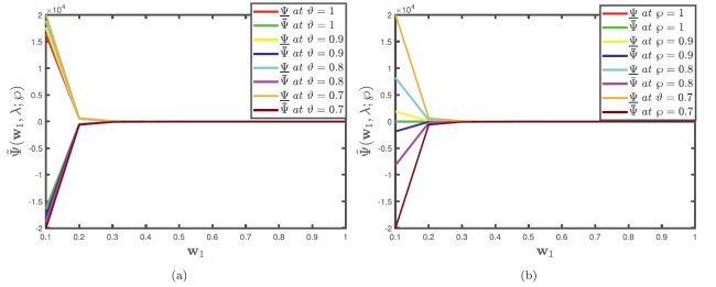
Fig. 4.2. (a) Solution profiles by Caputo fractional derivative of Problem 4.1 demonstrate (a) Lower and upper case solutions for different fractional orders with uncertainty parameter and λ=0.5. (b) Lower and upper case solutions for various uncertainties with and λ=0.5. |
Fig. 4.3 illustrates the analysis of Problem 4.1 under -differentiabilty of ABC fractional derivative (a) the two dimensional approximate solution with various fractional orders but fixed uncertain parameter (b) the two dimensional approximate solution with various uncertain parameters but fixed fractional order .
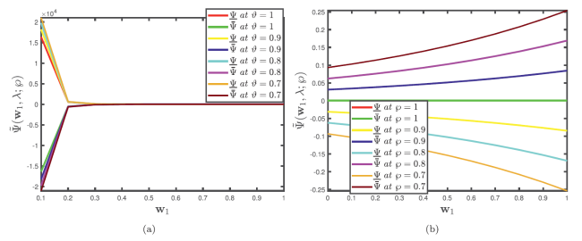
Fig. 4.3. Solution profiles by ABC fractional derivative of Problem 4.1 demonstrate (a) Lower and upper case solutions for different fractional orders with uncertainty parameter and λ=0.5. (b) Lower and upper case solutions for various uncertainties with and λ=0.5. |
Fig. 4.4 defines the comparison analysis of Problem 4.1 under -differentiabilty of Caputo and ABC fractional derivatives (a) 3D simulation (b) 2D simulation. At the third term approximation, the values of the numerical results of multiple grid points generated by the GHPTM are comparable to the values of the exact solution with high accuracy, indicating a high level of conformity with the two findings of different fractional operators with excellent convergence between them. Furthermore, by implementing inferential statistical testing, the proposed method will aid scientists working on magneto-acoustic waves occurring in plasma and fullid mechanics in assessing competency.
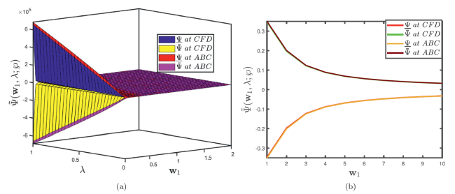
Fig. 4.4. Comparisons solution profiles by Caputo and ABC fractional derivative of Problem 4.1 demonstrates (a) three dimensional lower and upper case solutions, (b) two dimensional lower and upper case solutions, when and λ=0.5. |
Remark 4.1. Letting then the approximate solution of Problem 4.1 reduces to
Problem 4.2. Consider the nonlinear fuzzy fractional fifth order Kdv model:
$ \begin{array}{l} \frac{\partial^{\vartheta}}{\partial \lambda^{\vartheta}} \widetilde{\Psi}\left(\mathbf{w}_{1}, \lambda ; \wp\right)=\widetilde{\Psi} \odot \frac{\partial^{3}}{\partial \mathbf{w}_{1}^{3}} \widetilde{\Psi}\left(\mathbf{w}_{1}, \lambda ; \wp\right) \ominus \frac{\partial^{5}}{\partial \mathbf{w}_{1}^{5}} \widetilde{\Psi}\left(\mathbf{w}_{1}, \lambda ; \wp\right) \ominus \widetilde{\Psi}\left(\mathbf{w}_{1}, \lambda ; \wp\right) \\ \odot \frac{\partial}{\partial \mathbf{w}_{1}} \widetilde{\Psi}\left(\mathbf{w}_{1}, \lambda ; \wp\right) \end{array} $
subject to fuzzy ICs
$ \widetilde{\Psi}\left(\mathbf{w}_{1}, 0\right)=\widetilde{\Upsilon}(\wp) \odot \exp \left(\mathbf{w}_{1}\right) $
where $\widetilde{\Upsilon}(\wp)=[\underline{\Upsilon}(\wp), \bar{\Upsilon}(\wp)]=[\wp-1,1-\wp]$ for is fuzzy number.
The parameterized formulation of (4.6) is presented as
$ \left\{\begin{array}{l} \frac{\partial^{\vartheta}}{\partial \lambda^{\vartheta}} \underline{\Psi}\left(\mathbf{w}_{1}, \lambda ; \wp\right)=\underline{\Psi} \frac{\partial^{3}}{\partial \mathbf{w}_{1}^{3}} \underline{\Psi}\left(\mathbf{w}_{1}, \lambda ; \wp\right)-\frac{\partial^{5}}{\partial \mathbf{w}_{1}^{5}} \underline{\Psi}\left(\mathbf{w}_{1}, \lambda ; \wp\right)-\underline{\Psi}\left(\mathbf{w}_{1}, \lambda ; \wp\right) \frac{\partial}{\partial \mathbf{w}_{1}} \underline{\Psi}\left(\mathbf{w}_{1}, \lambda ; \wp\right), \\ \underline{\Psi}\left(\mathbf{w}_{1}, 0\right)=(\wp-1) \exp \left(\mathbf{w}_{1}\right) \\ \frac{\partial^{\vartheta}}{\partial \lambda^{\vartheta}} \bar{\Psi}\left(\mathbf{w}_{1}, \lambda ; \wp\right)=\bar{\Psi} \frac{\partial^{3}}{\partial \mathbf{w}_{1}^{3}} \bar{\Psi}\left(\mathbf{w}_{1}, \lambda ; \wp\right)-\frac{\partial^{5}}{\partial \mathbf{w}_{1}^{5}} \bar{\Psi}\left(\mathbf{w}_{1}, \lambda ; \wp\right) \\ -\bar{\Psi}\left(\mathbf{w}_{1}, \lambda ; \wp\right) \frac{\partial}{\partial \mathbf{w}_{1}} \bar{\Psi}\left(\mathbf{w}_{1}, \lambda ; \wp\right), \\ \bar{\Psi}\left(\mathbf{w}_{1}, 0\right)=(\wp-1) \exp \left(\mathbf{w}_{1}\right). \end{array}\right. $
Case I. Firstly, taking into consideration the CFD coupled with the generalized homotopy perturbation transform method on the first case of (4.3). In view of the process stated in Section 3, we have
$\begin{array}{l} \Phi^{\vartheta}\left(s_{1}\right) \mathbf{J}\left[\underline{\Psi}\left(\mathbf{w}_{1}, \lambda ; \wp\right)\right]-\Theta\left(s_{1}\right) \sum_{\kappa=0}^{q-1} \Phi^{\vartheta-1-\kappa}\left(s_{1}\right) \underline{\Psi}^{(\kappa)}\left(\mathbf{w}_{1}, 0 ; \wp\right) \\ =\mathbf{J}\left[\underline{\Psi} \frac{\partial^{3}}{\partial \mathbf{w}_{1}^{3}} \underline{\Psi}\left(\mathbf{w}_{1}, \lambda ; \wp\right)-\frac{\partial^{5}}{\partial \mathbf{w}_{1}^{5}} \underline{\Psi}\left(\mathbf{w}_{1}, \lambda ; \wp\right)-\underline{\Psi}\left(\mathbf{w}_{1}, \lambda ; \wp\right) \frac{\partial}{\partial \mathbf{w}_{1}} \underline{\Psi}\left(\mathbf{w}_{1}, \lambda ; \wp\right)\right]. \end{array}$
In view of fuzzy IC and making use of the inverse generalized integral transform implies
$\begin{aligned} \underline{\Psi}\left(\mathbf{w}_{1}, \lambda ; \wp\right) & =(\wp-1) \exp \left(\mathbf{w}_{1}\right) \\ & +\mathbf{J}^{-1}\left[\frac { 1 } { \Phi ^ { \vartheta } ( s _ { 1 } ) } \mathbf { J } \left[\underline{\Psi} \frac{\partial^{3}}{\partial \mathbf{w}_{1}^{3}} \underline{\Psi}\left(\mathbf{w}_{1}, \lambda ; \wp\right)-\frac{\partial^{5}}{\partial \mathbf{w}_{1}^{5}} \underline{\Psi}\left(\mathbf{w}_{1}, \lambda ; \wp\right)\right.\right. \\ & \left.\left.-\underline{\Psi}\left(\mathbf{w}_{1}, \lambda ; \wp\right) \frac{\partial}{\partial \mathbf{w}_{1}} \underline{\Psi}\left(\mathbf{w}_{1}, \lambda ; \wp\right)\right]\right]. \end{aligned}$
Now implementing the HPM, we have
$ \begin{array}{l} \sum_{\kappa=0}^{\infty} \eta^{\kappa} \underline{\Psi}_{\kappa}\left(\mathbf{w}_{1}, \lambda ; \wp\right)=(\wp-1) \exp \left(\mathbf{w}_{1}\right) \\ -\eta\left(\mathbf{J}^{-1}\left[\frac{1}{\Phi^{\vartheta}\left(s_{1}\right)} \mathbf{J}\left[\left(\sum_{\kappa=0}^{\infty} \eta^{\kappa} \underline{\Psi}_{\kappa}\left(\mathbf{w}_{1}, \lambda ; \wp\right)\right)_{5 \mathbf{w}_{1}}-\left(\sum_{\kappa=0}^{\infty} \eta^{\kappa} \underline{\mathscr{U}}_{\kappa}(\underline{\Psi})\right)\right]\right]\right). \end{array} $
$ \begin{array}{l} \underline{U}_{\kappa}\left(\underline{\Psi}_{1}\right. \\ =\left\{\begin{array}{l} \underline{\Psi}_{0}\left(\underline{\Psi}_{0}\right)_{3 \mathbf{w}_{1}}-\underline{\Psi}_{0}\left(\underline{\Psi}_{0}\right)_{\mathbf{w}_{1}}, \quad \kappa=0, \\ \underline{\Psi}_{1}\left(\underline{\Psi}_{0}\right)_{3 \mathbf{w}_{1}}+\underline{\Psi}_{0}\left(\underline{\Psi}_{1}\right)_{3 \mathbf{w}_{1}}-\underline{\Psi}_{1}\left(\underline{\Psi}_{0}\right)_{\mathbf{w}_{1}}-\underline{\Psi}_{0}\left(\underline{\Psi}_{0}\right)_{\mathbf{w}_{1}}, \quad \kappa=1, \\ \underline{\Psi}_{2}\left(\underline{\Psi}_{0}\right)_{3 \mathbf{w}_{1}}+\underline{\Psi}_{1}\left(\underline{\Psi}_{1}\right)_{3 \mathbf{w}_{1}}+\underline{\Psi}_{0}\left(\underline{\Psi}_{2}\right)_{3 \mathbf{w}_{1}}-\underline{\Psi}_{2}\left(\underline{\Psi}_{0}\right)_{\mathbf{w}_{1}}-\underline{\Psi}_{1}\left(\underline{\Psi}_{1}\right)_{\mathbf{w}_{1}} \\ -\underline{\Psi}_{0}\left(\underline{\Psi}_{2}\right)_{w_{1}}, \quad \kappa=2. \end{array}\right. \end{array} $
Equating the coefficients of the same powers of η, we have
$\begin{aligned} \eta^{0}: \underline{\Psi}_{0}\left(\mathbf{w}_{1}, \lambda ; \wp\right) & =(\wp-1) \exp \left(\mathbf{w}_{1}\right), \\ \eta^{1}: \underline{\Psi}_{1}\left(\mathbf{w}_{1}, \lambda ; \wp\right) & =-\mathbf{J}^{-1}\left[\frac{1}{\Phi^{\vartheta}\left(s_{1}\right)} \mathbf{J}\left[\left(\underline{\Psi}_{0}\left(\mathbf{w}_{1}, \lambda ; \wp\right)\right) 5 \mathbf{w}_{1}-\underline{\mathscr{U}}_{0}(\underline{\Psi})\right]\right]= \\ & -(\wp-1) \exp \left(\mathbf{w}_{1}\right) \frac{\lambda^{\vartheta}}{\Gamma(\vartheta+1)}, \\ \eta^{2}: \underline{\Psi}_{2}\left(\mathbf{w}_{1}, \lambda ; \wp\right) & =-\mathbf{J}^{-1}\left[\frac{1}{\Phi^{\vartheta}\left(s_{1}\right)} \mathbf{J}\left[\left(\underline{\Psi}_{1}\left(\mathbf{w}_{1}, \lambda ; \wp\right)\right) 5 \mathbf{w}_{1}-\underline{\mathscr{U}}_{1}(\underline{\Psi})\right]\right] \\ & =(\wp-1) \exp \left(\mathbf{w}_{1}\right) \frac{\lambda^{2 \vartheta}}{\Gamma(2 \vartheta+1)}, \\ \eta^{3}: \underline{\Psi}_{3}\left(\mathbf{w}_{1}, \lambda ; \wp\right) & =-\mathbf{J}^{-1}\left[\frac{1}{\Phi^{\vartheta}\left(s_{1}\right)} \mathbf{J}\left[\left(\underline{\Psi}_{3}\left(\mathbf{w}_{1}, \lambda ; \wp\right)\right) 5 \mathbf{w}_{1}-\underline{\mathscr{U}}_{2}(\underline{\Psi})\right]\right]= \\ & -(\wp-1) \exp \left(\mathbf{w}_{1}\right) \frac{\lambda^{3 \vartheta}}{\Gamma(3 \vartheta+1)}, \\ \vdots. & \end{aligned}$
The series form solution is presented as follows
$\widetilde{\Psi}\left(\mathbf{w}_{1}, \lambda ; \wp\right)=\widetilde{\Psi}_{0}\left(\mathbf{w}_{1}, \lambda ; \wp\right)+\widetilde{\Psi}_{1}\left(\mathbf{w}_{1}, \lambda ; \wp\right)+\widetilde{\Psi}_{2}\left(\mathbf{w}_{1}, \lambda ; \wp\right)+\widetilde{\Psi}_{3}\left(\mathbf{w}_{1}, \lambda ; \wp\right)+\ldots$
implies that
$\begin{array}{l} \underline{\Psi}\left(\mathbf{w}_{1}, \lambda ; \wp\right)=\underline{\Psi}_{0}\left(\mathbf{w}_{1}, \lambda ; \wp\right)+\underline{\Psi}_{1}\left(\mathbf{w}_{1}, \lambda ; \wp\right)+\underline{\Psi}_{2}\left(\mathbf{w}_{1}, \lambda ; \wp\right)+\underline{\Psi}_{3}\left(\mathbf{w}_{1}, \lambda ; \wp\right)+\ldots \\ \bar{\Psi}\left(\mathbf{w}_{1}, \lambda ; \wp\right)=\bar{\Psi}_{0}\left(\mathbf{w}_{1}, \lambda ; \wp\right)+\bar{\Psi}_{1}\left(\mathbf{w}_{1}, \lambda ; \wp\right)+\bar{\Psi}_{2}\left(\mathbf{w}_{1}, \lambda ; \wp\right)+\bar{\Psi}_{3}\left(\mathbf{w}_{1}, \lambda ; \wp\right)+\ldots \end{array}$
Finally, we have
$\begin{array}{ll} \underline{\Psi}\left(\mathbf{w}_{1}, \lambda ; \wp\right) & =(\wp-1) \exp \left(\mathbf{w}_{1}\right)\left[1-\frac{\lambda^{\vartheta}}{\Gamma(\vartheta+1)}+\frac{\lambda^{2 \vartheta}}{\Gamma(2 \vartheta+1)}-\frac{\lambda^{3 \vartheta}}{\Gamma(3 \vartheta+1)}+\ldots\right], \\ \bar{\Psi}\left(\mathbf{w}_{1}, \lambda ; \wp\right) & =(1-\wp) \exp \left(\mathbf{w}_{1}\right)\left[1-\frac{\lambda^{\vartheta}}{\Gamma(\vartheta+1)}+\frac{\lambda^{2 \vartheta}}{\Gamma(2 \vartheta+1)}-\frac{\lambda^{3 \vartheta}}{\Gamma(3 \vartheta+1)}+\ldots\right]. \end{array}$
Case 2. Now, we employ the fuzzy ABC derivative operator on the first first case of (4.3) as follows: In view of the process stated in Section 3, we have
$\begin{array}{l} \frac{\Phi^{\vartheta}\left(s_{1}\right) \mathbb{B}(\vartheta)}{\vartheta+(1-\vartheta) \Phi^{\vartheta}(s)}\left[\underline{\mathscr{U}}\left(\mathbf{w}_{1}, s_{1} ; \wp\right)-\frac{\Theta\left(s_{1}\right)}{\Phi(s)} \underline{\Psi}\left(\mathbf{w}_{1}, 0 ; \wp\right)\right] \\ =\mathbf{J}\left[\underline{\Psi} \frac{\partial^{3}}{\partial \mathbf{w}_{1}^{3}} \underline{\Psi}\left(\mathbf{w}_{1}, \lambda ; \wp\right)-\frac{\partial^{5}}{\partial \mathbf{w}_{1}^{5}} \underline{\Psi}\left(\mathbf{w}_{1}, \lambda ; \wp\right)-\underline{\Psi}\left(\mathbf{w}_{1}, \lambda ; \wp\right) \frac{\partial}{\partial \mathbf{w}_{1}} \underline{\Psi}\left(\mathbf{w}_{1}, \lambda ; \wp\right)\right]. \end{array}$
In view of fuzzy IC and making use of the inverse generalized integral transform implies
$\begin{aligned} \underline{\Psi}\left(\mathbf{w}_{1}, \lambda ; \wp\right)= & (\wp-1) \exp \left(\mathbf{w}_{1}\right)+\mathbf{J}^{-1}\left[\frac { \vartheta + ( 1 - \vartheta ) \Phi ^ { \vartheta } ( s ) } { \Phi ^ { \vartheta } ( s _ { 1 } ) \mathbb { B } ( \vartheta ) } \mathbf { J } \left[\underline{\Psi} \frac{\partial^{3}}{\partial \mathbf{w}_{1}^{3}} \underline{\Psi}\left(\mathbf{w}_{1}, \lambda ; \wp\right)\right.\right. \\ - & \frac{\partial^{5}}{\partial \mathbf{w}_{1}^{5}} \underline{\Psi}\left(\mathbf{w}_{1}, \lambda ; \wp\right) \\ & \left.\left.-\underline{\Psi}\left(\mathbf{w}_{1}, \lambda ; \wp\right) \frac{\partial}{\partial \mathbf{w}_{1}} \underline{\Psi}\left(\mathbf{w}_{1}, \lambda ; \wp\right)\right]\right]. \end{aligned}$
Now implementing the HPM, we have
$\begin{aligned} \sum_{\kappa=0}^{\infty} \eta^{\kappa} \underline{\Psi}_{\kappa}\left(\mathbf{w}_{1}, \lambda ; \wp\right) & =(\wp-1) \exp \left(\mathbf{w}_{1}\right) \\ & +\eta\left(\mathbf{J}^{-1}\left[\frac{\vartheta+(1-\vartheta) \Phi^{\vartheta}(s)}{\Phi^{\vartheta}\left(s_{1}\right) \mathbb{B}(\vartheta)} \mathbf{J}\left[\left(\sum_{\kappa=0}^{\infty} \eta^{\kappa} \underline{\Psi}_{\kappa}\left(\mathbf{w}_{1}, \lambda ; \wp\right)\right) 5_{1}-\left(\sum_{\kappa=0}^{\infty} \eta^{\kappa} \underline{\mathscr{U}}_{\kappa}(\underline{\Psi})\right)\right]\right]\right). \end{aligned}$
By the virtue of (4.10), we can calculate the following iterative terms by equating the coefficients of the same powers of η, we have
$\begin{aligned} \eta^{0}: \underline{\Psi}_{0}\left(\mathbf{w}_{1}, \lambda ; \wp\right) & =(\wp-1) \exp \left(\mathbf{w}_{1}\right), \\ \eta^{1}: \underline{\Psi}_{1}\left(\mathbf{w}_{1}, \lambda ; \wp\right) & =-\mathbf{J}^{-1}\left[\frac{\vartheta+(1-\vartheta) \Phi^{\vartheta}(s)}{\Phi^{\vartheta}\left(s_{1}\right) \mathbb{B}(\vartheta)} \mathbf{J}\left[\left(\underline{\Psi}_{0}\left(\mathbf{w}_{1}, \lambda ; \wp\right)\right) 5 \mathbf{w}_{1}-\underline{\mathscr{U}}_{0}(\underline{\Psi})\right]\right] \\ & =-(\wp-1) \exp \left(\mathbf{w}_{1}\right)\left(\frac{\vartheta \lambda^{\vartheta}}{\Gamma(\vartheta+1)}+(1-\vartheta)\right), \\ \eta^{2}: \underline{\Psi}_{2}\left(\mathbf{w}_{1}, \lambda ; \wp\right) & =-\mathbf{J}^{-1}\left[\frac{\vartheta+(1-\vartheta) \Phi^{\vartheta}(s)}{\Phi^{\vartheta}\left(s_{1}\right) \mathbb{B}(\vartheta)} \mathbf{J}\left[\left(\underline{\Psi}_{1}\left(\mathbf{w}_{1}, \lambda ; \wp\right)\right) 5 \mathbf{w}_{1}-\underline{\mathscr{U}}_{1}(\underline{\Psi})\right]\right] \\ & =(\wp-1) \exp \left(\mathbf{w}_{1}\right)\left(\frac{\vartheta^{2} \lambda^{2 \vartheta}}{\Gamma(2 \vartheta+1)}+2 \vartheta(1-\vartheta) \frac{\lambda^{\vartheta}}{\Gamma(\vartheta+1)}+(1-\vartheta)^{2}\right), \\ \eta^{3}: \underline{\Psi}_{3}\left(\mathbf{w}_{1}, \lambda ; \wp\right) & \left.=-\mathbf{J}^{-1}\left[\frac{\vartheta+(1-\vartheta) \Phi^{\vartheta}(s)}{\Phi^{\vartheta}\left(s_{1}\right) \mathbb{B}(\vartheta)} \mathbf{J}\left[\left(\underline{\Psi}_{2}\left(\mathbf{w}_{1}, \lambda ; \wp\right)\right) 5 \mathbf{w}_{1}-\underline{\mathscr{U}}_{2}(\underline{\Psi})\right]\right]\right] \\ & =-(\wp-1) \exp \left(\mathbf{w}_{1}\right)\left(\frac{\vartheta^{3} \lambda^{3 \vartheta}}{\Gamma(3 \vartheta+1)}+3 \vartheta^{2}(1-\vartheta) \frac{\lambda^{2 \vartheta}}{\Gamma(2 \vartheta+1)}+3 \vartheta(1-\vartheta)^{2} \frac{\lambda^{\vartheta}}{\Gamma(\vartheta+1)}\right. \\ & \left.+(1-\vartheta)^{3}\right), \\ \vdots. & \end{aligned}$
The series form solution is presented as follows:
$\widetilde{\Psi}\left(\mathbf{w}_{1}, \lambda ; \wp\right)=\widetilde{\Psi}_{0}\left(\mathbf{w}_{1}, \lambda ; \wp\right)+\widetilde{\Psi}_{1}\left(\mathbf{w}_{1}, \lambda ; \wp\right)+\widetilde{\Psi}_{2}\left(\mathbf{w}_{1}, \lambda ; \wp\right)+\widetilde{\Psi}_{3}\left(\mathbf{w}_{1}, \lambda ; \wp\right)+\ldots,$
implies that
$\begin{array}{l} \underline{\Psi}\left(\mathbf{w}_{1}, \lambda ; \wp\right)=\underline{\Psi}_{0}\left(\mathbf{w}_{1}, \lambda ; \wp\right)+\underline{\Psi}_{1}\left(\mathbf{w}_{1}, \lambda ; \wp\right)+\underline{\Psi}_{2}\left(\mathbf{w}_{1}, \lambda ; \wp\right)+\underline{\Psi}_{3}\left(\mathbf{w}_{1}, \lambda ; \wp\right)+\ldots \\ \bar{\Psi}\left(\mathbf{w}_{1}, \lambda ; \wp\right)=\bar{\Psi}_{0}\left(\mathbf{w}_{1}, \lambda ; \wp\right)+\bar{\Psi}_{1}\left(\mathbf{w}_{1}, \lambda ; \wp\right)+\bar{\Psi}_{2}\left(\mathbf{w}_{1}, \lambda ; \wp\right)+\bar{\Psi}_{3}\left(\mathbf{w}_{1}, \lambda ; \wp\right)+\ldots \end{array}$
Finally, we have
$\begin{aligned} \underline{\Psi}\left(\mathbf{w}_{1}, \lambda ; \wp\right) & =(\wp-1) \exp \left(\mathbf{w}_{1}\right)\left[2-4 \alpha+4 \alpha^{2}-\alpha^{3}+\left(3 \alpha^{3}-8 \alpha^{2}+4 \alpha\right) \frac{\lambda^{\vartheta}}{\Gamma(\vartheta+1)}\right. \\ & \left.+\alpha^{2}(2-3 \alpha) \frac{\lambda^{2 \vartheta}}{\Gamma(2 \vartheta+1)}-\alpha^{3} \frac{\lambda^{3 \vartheta}}{\Gamma(3 \vartheta+1)} \ldots\right], \\ \bar{\Psi}\left(\mathbf{w}_{1}, \lambda ; \wp\right) & =(1-\wp) \exp \left(\mathbf{w}_{1}\right)\left[2-4 \alpha+4 \alpha^{2}-\alpha^{3}+\left(3 \alpha^{3}-8 \alpha^{2}+4 \alpha\right) \frac{\lambda^{\vartheta}}{\Gamma(\vartheta+1)}\right. \\ & \left.+\alpha^{2}(2-3 \alpha) \frac{\lambda^{2 \vartheta}}{\Gamma(2 \vartheta+1)}-\alpha^{3} \frac{\lambda^{3 \vartheta}}{\Gamma(3 \vartheta+1)} \ldots\right]. \end{aligned}$
In this analysis, we compared the lower and upper accuracies of and the HPM solutions [72] in Table 1. We assumed the fractional order to be when with varying values of and λ. Where, values written for HPM solution have been achieved by reference [72]. In Table2, we showed the absolute error between different values of and when and employing JHPTM for the non-homogeneous fifth order KdV equation, showing how the approximate solution is compared with the exact solution.
Table 4. 1. The exact, the lower and upper accuracies via and the lower and upper accuracies via solutions of Example 4.2 with varying values of and λ in comparison with the solution profile of [72] obtained by homotopy perturbation method. |
| Empty Cell | λ | $\underline{\Psi}_{C F D}$ | $\bar{\Psi}_{C F D}$ | $\underline{\Psi}_{A B C}$ | $\bar{\Psi}_{A B C}$ | Ψ [72] | Exact | Empty Cell | |
|---|---|---|---|---|---|---|---|---|---|
| 0.1 | -1.094119307 | 1.094119307 | -1.094119307 | 0.8958123558 | 1.105171018 | 1.105170918 | |||
| 0.2 | -0.9900031196 | 0.9900031196 | -0.9900031196 | 0.9900031196 | 1.000003152 | 1.00000000 | |||
| 0.2 | 0.3 | -0.8958123558 | 0.8958123558 | -0.8958123558 | 0.8958123558 | 0.9048609657 | 0.9048374180 | ||
| 0.4 | -0.8106401246 | 0.8106401246 | -0.8106401246 | 0.8106401246 | 0.8188284089 | 0.8187307531 | |||
| 0.5 | -0.7337004534 | 0.7337004534 | -0.7337004534 | 0.7337004534 | 0.7411115693 | 0.7408182207 | |||
| 0.1 | -1.336360341 | 1.336360341 | -1.336360341 | 1.336360341 | 1.349858930 | 1.349858808 | |||
| 0.2 | -1.209192542 | 1.209192542 | -1.209192542 | 1.209192542 | 1.221406607 | 1.221402758 | |||
| 0.4 | 0.3 | -1.094147683 | 1.094147683 | -1.094147683 | 1.094147683 | 1.105199680 | 1.105170918 | ||
| 0.4 | -0.9901180848 | 0.9901180848 | -0.9901180848 | 0.9901180848 | 1.000119278 | 1.00000000 | |||
| 0.5 | -0.8961437581 | 0.8961437581 | -0.8961437581 | 0.8961437581 | 0.9051957152 | 0.9048374180 | |||
| 0.1 | -1.632234205 | 1.632234205 | -1.632234205 | 1.632234205 | 1.648721420 | 1.648721271 | |||
| 0.2 | -1.476911105 | 1.476911105 | -1.476911105 | 1.476911105 | 1.491829399 | 1.491824698 | |||
| 0.6 | 0.3 | -1.336394997 | 1.336394997 | -1.336394997 | 1.336394997 | 1.349893936 | 1.349858808 | ||
| 0.4 | -1.209332959 | 1.209332959 | -1.209332959 | 1.209332959 | 1.221548443 | 1.221402758 | |||
| 0.5 | -1.094552457 | 1.094552457 | -1.094552457 | 1.094552457 | 1.105608543 | 1.105170918 | |||
| 0.1 | -1.993615361 | 1.993615361 | -1.993615361 | -1.993615361 | 2.013752890 | 2.013752707 | |||
| 0.2 | -1.803903297 | 1.803903297 | -1.803903297 | -1.803903297 | 1.822124542 | 1.822118800 | |||
| 0.8 | 0.3 | -1.632276536 | 1.632276536 | -1.632276536 | 1.632276536 | 1.648764178 | 1.648721271 | ||
| 0.4 | -1.477082612 | 1.477082612 | -1.477082612 | 1.477082612 | 1.492002638 | 1.491824698 | |||
| 0.5 | -1.336889391 | 1.336889391 | -1.336889391 | 1.336889391 | 1.350393324 | 1.349858808 | |||
| 0.1 | -2.4389324561 | 2.4389324561 | -2.4389324561 | 2.4389324561 | 2.449603111 | 2.459603111 | |||
| 0.2 | -2.203292463 | 2.203292463 | -2.203292463 | 2.203292463 | 2.225547944 | 2.225540928 | |||
| 1.0 | 0.3 | -1.993667063 | 1.993667063 | -1.993667063 | 1.993667063 | 2.013805114 | 2.013752707 | ||
| 0.4 | -1.804112776 | 1.804112776 | -1.804112776 | 1.804112776 | 1.822336137 | 1.822118800 | |||
| 0.5 | -1.632880389 | 1.632880389 | -1.632880389 | 1.632880389 | 1.649374132 | 1.648721271 |
Table 4. 2. The absolute error analysis among HPM [72], the absolute error of the lower and upper accuracies of and the lower and upper accuracies of of Example 4.2 for approximated results of at with varying values of and λ. |
| Empty Cell | λ | EHPM | $E_{\Psi} \text { for } C F D$ | $\begin{array}{c} E_{\bar{\Psi}} \text { for } \\ C F D \end{array}$ | $E_{\Psi} \text { for } A B C$ | $ E_{\bar{\Psi}} for {A B C}$ | |
|---|---|---|---|---|---|---|---|
| 0.1 | 1.00000×10⁻⁷ | 2.19929× 100 | 1.10516×10⁻² | 2.19929× 100 | 1.10516×10⁻² | ||
| 0.2 | 3.15200×10⁻⁶ | 1.99000× 100 | 9.99688×10⁻³ | 1.99000× 100 | 9.99688×10⁻³ | ||
| 0.2 | 0.3 | 2.35477×10⁻⁵ | 1.80065 × 100 | 9.02506×10⁻³ | 1.80065× 100 | 9.02506×10⁻³ | |
| 0.4 | 9.76558×10⁻⁵ | 1.62937 × 100 | 8.09063×10⁻³ | 1.62937× 100 | 8.09063×10⁻³ | ||
| 0.5 | 2.93349×10⁻⁴ | 1.47452× 100 | 7.11777×10⁻³ | 1.47452× 100 | 7.11777×10⁻³ | ||
| 0.1 | 1.22000×10⁻⁷ | 2.68622× 100 | 1.34985×10⁻² | 2.68622× 100 | 1.34985×10⁻² | ||
| 0.2 | 3.84900×10⁻⁶ | 2.43060× 10 0 | 1.22102×10⁻² | 2.43060× 100 | 1.22102×10⁻² | ||
| 0.4 | 0.3 | 2.87620×10⁻⁵ | 2.19932× 100 | 1.10232×10⁻² | 2.19932× 100 | 1.10232×10⁻² | |
| 0.4 | 1.19278×10⁻⁴ | 1.99012× 100 | 9.88192×10⁻³ | 1.99012× 100 | 9.88192×10⁻³ | ||
| 0.5 | 3.58297×10⁻⁴ | 1.80098× 100 | 8.69366×10⁻³ | 1.80098× 100 | 8.69366×10⁻³ | ||
| 0.1 | 1.49000×10⁻⁷ | 3.28096 × 10 0 | 1.64871×10⁻² | 3.28096× 100 | 1.64871 ×10⁻² | ||
| 0.2 | 4.70100×10⁻⁶ | 2.96874 × 10 0 | 1.49136×10⁻² | 2.96874× 100 | 1.49136×10⁻² | ||
| 0.6 | 0.3 | 3.51280×10⁻⁵ | 2.68625× 100 | 1.34638×10⁻² | 2.68625× 100 | 1.34638×10⁻² | |
| 0.4 | 1.45685×10⁻⁴ | 2.43074× 10 0 | 1.20698×10⁻² | 2.43074× 100 | 1.20698×10⁻² | ||
| 0.5 | 4.37625×10⁻⁴ | 2.19972× 100 | 1.06185×10⁻² | 2.19972× 100 | 1.06185×10⁻² | ||
| 0.1 | 1.83000×10⁻⁷ | 4.00737× 100 | 2.01373×10⁻² | 4.00737× 100 | 2.01373×10⁻² | ||
| 0.2 | 5.74200*×10−6 | 3.62602× 100 | 1.82155×10⁻² | 3.62602× 100 | 1.82155×10⁻² | ||
| 0.8 | 0.3 | 4.29070×10⁻⁵ | 3.28100× 100 | 1.64447×10⁻² | 3.28100× 100 | 1.64447×10⁻² | |
| 0.8 | 1.77940×10⁻⁴ | 2.96891× 100 | 1.47421×10⁻² | 2.96891× 100 | 1.47421×10⁻² | ||
| 0.5 | 5.34516×10⁻⁴ | 2.68675× 100 | 1.29694×10⁻² | 2.68675× 100 | 1.29694×10⁻² | ||
| 0.1 | 2.23000×10⁻⁷ | 4.89461× 100 | 2.45958×10⁻² | 4.89461× 100 | 2.45958×10⁻² | ||
| 0.2 | 7.01600×10⁻⁶ | 4.42883× 100 | 2.22485×10⁻² | 4.42883× 100 | 2.22485×10⁻² | ||
| 1.0 | 0.3 | 5.24070×10⁻⁵ | 4.00742× 100 | 2.00856×10⁻² | 4.00742× 100 | 2.00856×10⁻² | |
| 0.4 | 2.17337×10⁻⁴ | 3.62623× 100 | 1.80060×10⁻² | 3.62623× 100 | 1.80060×10⁻² | ||
| 0.5 | 6.52861×10⁻⁴ | 3.28160× 100 | 1.58409×10⁻² | 3.28160× 100 | 1.58409×10⁻² |
From Fig. 4.5 represents the analysis of Problem 4.2 (a) the lower and upper accuracy for the approximate solutions under -differentiabilty of CFD when (b) the lower and upper accuracy for the approximate solutions under -differentiabilty of CFD when It is worth mentioning that as the accuracies increase, the order of approximations increases.
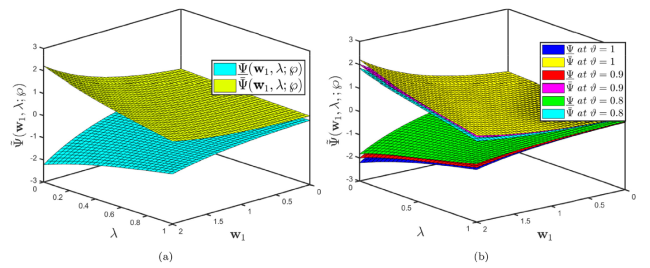
Fig. 4.5. Solution profiles of Problem 4.2 demonstrate (a) Lower and upper case solutions for (b) Lower and upper case solutions for ϑ=1,0.9, and 0.8. |
Fig. 4.6 displays the analysis of Problem 4.2 under -differentiabilty of CFD (a) the two dimensional approximate solution with various fractional orders but fixed uncertain parameters (b) the two dimensional approximate solution with various uncertain parameters but fixed fractional order
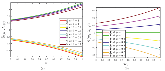
Fig. 4.6. Solution profiles by Caputo fractional derivative of Problem 4.2 demonstrate (a) Lower and upper case solutions for different fractional orders with uncertainty parameter and λ=0.5. (b) Lower and upper case solutions for various uncertainties with and λ=0.5. |
Fig. 4.7 illustrates the analysis of Problem 4.2 under -differentiabilty of ABC fractional derivative (a) the two dimensional approximate solution with various fractional orders but fixed uncertain parameter (b) the two dimensional approximate solution with various uncertain parameters but fixed fractional order
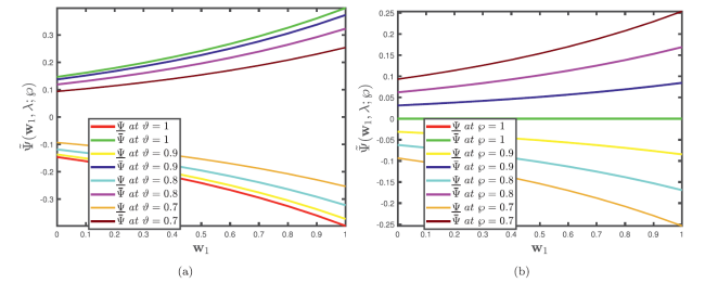
Fig. 4.7. Solution profiles by ABC fractional derivative of Problem 4.2 demonstrate (a) Lower and upper case solutions for different fractional orders with uncertainty parameter and λ=0.5. (b) Lower and upper case solutions for various uncertainties with and λ=0.5. |
Fig. 4.8 defines the comparison analysis of Problem 4.2 under -differentiabilty of Caputo and ABC fractional derivatives (a) 3D simulation (b) 2D simulation.
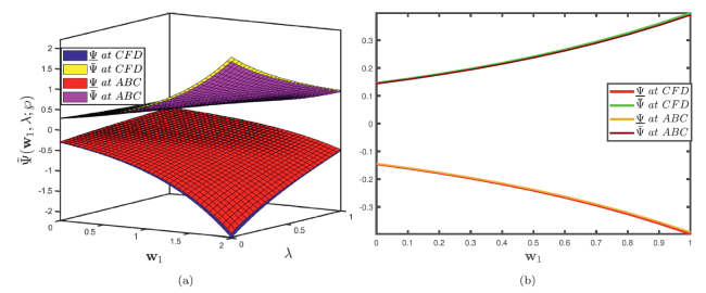
Fig. 4.8. Comparisons solution profiles by Caputo and ABC fractional derivative of Problem 4.1 demonstrates (a) three dimensional lower and upper case solutions, (b) two dimensional lower and upper case solutions, when and λ=0.5. |
At the third term approximation, the values of the numerical results of multiple grid points generated by the GHPTM are comparable to the values of the exact solution with high accuracy, indicating a high level of conformity with the two findings of different fractional operators with excellent convergence between them. Furthermore, by implementing inferential statistical testing, the proposed method will aid scientists working on magneto-acoustic waves occurring in plasma and fullid mechanics in assessing competency.
Remark 4.2. Letting $\underline{\Upsilon}(\wp)=\bar{\Upsilon}(\wp)=1$, then the approximate solution of Problem 4.2 reduces to.
Problem 4.3. Consider the fuzzy fractional dispersive KdV model:
$ \frac{\partial^{\vartheta}}{\partial \lambda^{\vartheta}} \widetilde{\Psi}\left(\mathbf{w}_{1}, \lambda ; \wp\right)=\ominus \frac{\partial^{3}}{\partial \mathbf{w}_{1}^{3}} \widetilde{\Psi}\left(\mathbf{w}_{1}, \lambda ; \wp\right) \ominus 2 \ominus \frac{\partial}{\partial \mathbf{w}_{1}} \widetilde{\Psi}\left(\mathbf{w}_{1}, \lambda ; \wp\right) $
subject to fuzzy ICs
$ \widetilde{\Psi}\left(\mathbf{w}_{1}, 0\right)=\widetilde{\Upsilon}(\wp) \odot \sin \left(\mathbf{w}_{1}\right) $
where $\widetilde{\Upsilon}(\wp)=[\underline{\Upsilon}(\wp), \bar{\Upsilon}(\wp)]=[\wp-1,1-\wp]$ for is fuzzy number.
The parameterized formulation of (4.11) is presented as
$ \left\{\begin{array}{l} \frac{\partial^{\vartheta}}{\partial \lambda^{\vartheta}} \underline{\Psi}\left(\mathbf{w}_{1}, \lambda ; \wp\right)=-\frac{\partial^{3}}{\partial \mathbf{w}_{1}^{3}} \Psi\left(\mathbf{w}_{1}, \lambda ; \wp\right)-2 \frac{\partial}{\partial \mathbf{w}_{1}} \underline{\Psi}\left(\mathbf{w}_{1}, \lambda ; \wp\right), \\ \underline{\Psi}\left(\mathbf{w}_{1}, 0\right)=(\wp-1) \sin \left(\mathbf{w}_{1}\right) \\ \frac{\partial^{\vartheta}}{\partial \lambda^{\vartheta}} \bar{\Psi}\left(\mathbf{w}_{1}, \lambda ; \wp\right)=-\frac{\partial^{3}}{\partial \mathbf{w}_{1}^{3}} \underline{\Psi}\left(\mathbf{w}_{1}, \lambda ; \wp\right)-2 \frac{\partial}{\partial \mathbf{w}_{1}} \underline{\Psi}\left(\mathbf{w}_{1}, \lambda ; \wp\right), \\ \bar{\Psi}\left(\mathbf{w}_{1}, 0\right)=(\wp-1) \sin \left(\mathbf{w}_{1}\right). \end{array}\right. $
Case I. Firstly, taking into consideration the CFD coupled with the generalized homotopy perturbation transform method on the first case of (4.3).
In view of the process stated in Section 3, we have
$\begin{array}{l} \Phi^{\vartheta}\left(s_{1}\right) \mathbf{J}\left[\underline{\Psi}\left(\mathbf{w}_{1}, \lambda ; \wp\right)\right]-\Theta\left(s_{1}\right) \sum_{\kappa=0}^{q-1} \Phi^{\vartheta-1-\kappa}\left(s_{1}\right) \underline{\Psi}^{(\kappa)}\left(\mathbf{w}_{1}, 0 ; \wp\right) \\ =\mathbf{J}\left[-\frac{\partial^{3}}{\partial \mathbf{w}_{1}^{3}} \underline{\Psi}\left(\mathbf{w}_{1}, \lambda ; \wp\right)-2 \frac{\partial}{\partial \mathbf{w}_{1}} \underline{\Psi}\left(\mathbf{w}_{1}, \lambda ; \wp\right)\right]. \end{array}$
In view of fuzzy IC and making use of the inverse generalized integral transform implies
$\begin{array}{l} \underline{\Psi}\left(\mathbf{w}_{1}, \lambda ; \wp\right)=(\wp-1) \sin \left(\mathbf{w}_{1}\right) \\ +\mathbf{J}^{-1}\left[\frac{1}{\Phi^{\vartheta}\left(s_{1}\right)} \mathbf{J}\left[-\frac{\partial^{3}}{\partial \mathbf{w}_{1}^{3}} \underline{\Psi}\left(\mathbf{w}_{1}, \lambda ; \wp\right)-2 \frac{\partial}{\partial \mathbf{w}_{1}} \underline{\Psi}\left(\mathbf{w}_{1}, \lambda ; \wp\right)\right]\right]. \end{array}$
Now implementing the HPM, we have
$\begin{aligned} \sum_{\kappa=0}^{\infty} \eta^{\kappa} \underline{\Psi}_{\kappa}\left(\mathbf{w}_{1}, \lambda ; \wp\right)= & \wp-1) \sin \left(\mathbf{w}_{1}\right) \\ & -\eta\left(\mathbf{J}^{-1}\left[\frac{1}{\Phi^{\vartheta}\left(s_{1}\right)} \mathbf{J}\left[\left(\sum_{\kappa=0}^{\infty} \eta^{\kappa} \underline{\Psi}_{\kappa}\left(\mathbf{w}_{1}, \lambda ; \wp\right)\right) 3 \mathbf{w}_{1}+2\left(\sum_{\kappa=0}^{\infty} \eta^{\kappa} \underline{\Psi}_{\kappa}\left(\mathbf{w}_{1}, \lambda ; \wp\right)\right) \mathbf{w}_{1}\right]\right]\right). \end{aligned}$
Equating the coefficients of the same powers of η, we have
$\begin{aligned} \eta^{0}: \underline{\Psi}_{0}\left(\mathbf{w}_{1}, \lambda ; \wp\right) & =(\wp-1) \sin \left(\mathbf{w}_{1}\right) \\ \eta^{1}: \underline{\Psi}_{1}\left(\mathbf{w}_{1}, \lambda ; \wp\right) & =-\mathbf{J}^{-1}\left[\frac{1}{\Phi^{\vartheta}\left(s_{1}\right)} \mathbf{J}\left[\left(\underline{\Psi}_{0}\left(\mathbf{w}_{1}, \lambda ; \wp\right)\right) 3 \mathbf{w}_{1}+2\left(\underline{\Psi}_{0}\left(\mathbf{w}_{1}, \lambda ; \wp\right)\right) \mathbf{w}_{1}\right]\right]= \\ & -(\wp-1) \cos \left(\mathbf{w}_{1}\right) \frac{\lambda^{\vartheta}}{\Gamma(\vartheta+1)}, \\ \eta^{2}: \underline{\Psi}_{2}\left(\mathbf{w}_{1}, \lambda ; \wp\right) & =-\mathbf{J}^{-1}\left[\frac{1}{\Phi^{\vartheta}\left(s_{1}\right)} \mathbf{J}\left[\left(\underline{\Psi}_{1}\left(\mathbf{w}_{1}, \lambda ; \wp\right)\right) 3 \mathbf{w}_{1}+2\left(\underline{\Psi}_{1}\left(\mathbf{w}_{1}, \lambda ; \wp\right)\right) \mathbf{w}_{1}\right]\right]= \\ & -(\wp-1) \sin \left(\mathbf{w}_{1}\right) \frac{\lambda^{2 \vartheta}}{\Gamma(2 \vartheta+1)}, \\ \eta^{3}: \underline{\Psi}_{3}\left(\mathbf{w}_{1}, \lambda ; \wp\right) & =-\mathbf{J}^{-1}\left[\frac{1}{\Phi^{\vartheta}\left(s_{1}\right)} \mathbf{J}\left[\left(\underline{\Psi}_{2}\left(\mathbf{w}_{1}, \lambda ; \wp\right)\right) 3 \mathbf{w}_{1}+2\left(\underline{\Psi}_{2}\left(\mathbf{w}_{1}, \lambda ; \wp\right)\right) \mathbf{w}_{1}\right]\right] \\ & =(\wp-1) \cos \left(\mathbf{w}_{1}\right) \frac{\lambda^{3 \vartheta}}{\Gamma(3 \vartheta+1)}, \\ \vdots. & \end{aligned}$
The series form solution is presented as follows
$\widetilde{\Psi}\left(\mathbf{w}_{1}, \lambda ; \wp\right)=\widetilde{\Psi}_{0}\left(\mathbf{w}_{1}, \lambda ; \wp\right)+\widetilde{\Psi}_{1}\left(\mathbf{w}_{1}, \lambda ; \wp\right)+\widetilde{\Psi}_{2}\left(\mathbf{w}_{1}, \lambda ; \wp\right)+\widetilde{\Psi}_{3}\left(\mathbf{w}_{1}, \lambda ; \wp\right)+\ldots,$
implies that
$\begin{array}{l} \underline{\Psi}\left(\mathbf{w}_{1}, \lambda ; \wp\right)=\underline{\Psi}_{0}\left(\mathbf{w}_{1}, \lambda ; \wp\right)+\underline{\Psi}_{1}\left(\mathbf{w}_{1}, \lambda ; \wp\right)+\underline{\Psi}_{2}\left(\mathbf{w}_{1}, \lambda ; \wp\right)+\underline{\Psi}_{3}\left(\mathbf{w}_{1}, \lambda ; \wp\right)+\ldots, \\ \bar{\Psi}\left(\mathbf{w}_{1}, \lambda ; \wp\right)=\bar{\Psi}_{0}\left(\mathbf{w}_{1}, \lambda ; \wp\right)+\bar{\Psi}_{1}\left(\mathbf{w}_{1}, \lambda ; \wp\right)+\bar{\Psi}_{2}\left(\mathbf{w}_{1}, \lambda ; \wp\right)+\bar{\Psi}_{3}\left(\mathbf{w}_{1}, \lambda ; \wp\right)+\ldots \\ \end{array}$
Finally, we have
$\begin{aligned} \underline{\Psi}\left(\mathbf{w}_{1}, \lambda ; \wp\right)= & (\wp-1) \sin \left(\mathbf{w}_{1}\right)\left[1-\frac{\lambda^{2 \vartheta}}{\Gamma(2 \vartheta+1)}+\frac{\lambda^{4 \vartheta}}{\Gamma(4 \vartheta+1)}-\ldots\right] \\ & -(\wp-1) \cos \left(\mathbf{w}_{1}\right)\left[\frac{\lambda^{\vartheta}}{\Gamma(\vartheta+1)}-\frac{\lambda^{3 \vartheta}}{\Gamma(3 \vartheta+1)}+\frac{\lambda^{5 \vartheta}}{\Gamma(5 \vartheta+1)}-\ldots\right], \\ \bar{\Psi}\left(\mathbf{w}_{1}, \lambda ; \wp\right)= & (1-\wp) \sin \left(\mathbf{w}_{1}\right)\left[1-\frac{\lambda^{2 \vartheta}}{\Gamma(2 \vartheta+1)}+\frac{\lambda^{4 \vartheta}}{\Gamma(4 \vartheta+1)}-\ldots\right] \\ & -(1-\wp) \cos \left(\mathbf{w}_{1}\right)\left[\frac{\lambda^{\vartheta}}{\Gamma(\vartheta+1)}-\frac{\lambda^{3 \vartheta}}{\Gamma(3 \vartheta+1)}+\frac{\lambda^{5 \vartheta}}{\Gamma(5 \vartheta+1)}-\ldots\right]. \end{aligned}$
Case 2. Now, we employ the fuzzy ABC derivative operator on the first first case of (4.3) as follows:
In view of the process stated in Section 3, we have
$\begin{array}{l} \frac{\Phi^{\vartheta}\left(s_{1}\right) \mathbb{B}(\vartheta)}{\vartheta+(1-\vartheta) \Phi^{\vartheta}(s)}\left[\underline{U}\left(\mathbf{w}_{1}, s_{1} ; \wp\right)-\frac{\Theta\left(s_{1}\right)}{\Phi(s)} \underline{\Psi}\left(\mathbf{w}_{1}, 0 ; \wp\right)\right] \\ =\mathbf{J}\left[-\frac{\partial^{3}}{\partial \mathbf{w}_{1}^{3}} \underline{\Psi}\left(\mathbf{w}_{1}, \lambda ; \wp\right)-2 \frac{\partial}{\partial \mathbf{w}_{1}} \underline{\Psi}\left(\mathbf{w}_{1}, \lambda ; \wp\right)\right]. \end{array}$
In view of fuzzy IC and making use of the inverse generalized integral transform implies
$\begin{array}{l} \underline{\Psi}\left(\mathbf{w}_{1}, \lambda ; \wp\right)=(\wp-1) \sin \left(\mathbf{w}_{1}\right)+\mathbf{J}^{-1}\left[\frac { \vartheta + ( 1 - \vartheta ) \Phi ^ { \vartheta } ( s ) } { \Phi ^ { \vartheta } ( s _ { 1 } ) \mathbb { B } ( \vartheta ) } \mathbf { J } \left[-\frac{\partial^{3}}{\partial \mathbf{w}_{1}^{3}} \underline{\Psi}\left(\mathbf{w}_{1}, \lambda ; \wp\right)\right.\right. \\ \left.\left.-2 \frac{\partial}{\partial \mathbf{w}_{1}} \underline{\Psi}\left(\mathbf{w}_{1}, \lambda ; \wp\right)\right]\right]. \end{array}$
Now implementing the HPM, we have
$\begin{aligned} \sum_{\kappa=0}^{\infty} \eta^{\kappa} \underline{\Psi}_{\kappa}\left(\mathbf{w}_{1}, \lambda ; \wp\right)= & (-1) \sin \left(\mathbf{w}_{1}\right)-\eta\left(\mathbf { J } ^ { - 1 } \left[\frac { \vartheta + ( 1 - \vartheta ) \Phi ^ { \vartheta } ( s ) } { \Phi ^ { \vartheta } ( s _ { 1 } ) \mathbb { B } ( \vartheta ) } \mathbf { J } \left[\left(\sum_{\kappa=0}^{\infty} \eta^{\kappa} \underline{\Psi}_{\kappa}\left(\mathbf{w}_{1}, \lambda ; \wp\right)\right) 3 \mathbf{w}_{1}\right.\right.\right. \\ & \left.\left.\left.+2\left(\sum_{\kappa=0}^{\infty} \eta^{\kappa} \underline{\Psi}_{\kappa}\left(\mathbf{w}_{1}, \lambda ; \wp\right)\right) \mathbf{w}_{1}\right]\right]\right). \end{aligned}$
Equating the coefficients of the same powers of η, we have
$\begin{aligned} \eta^{0}: \underline{\Psi}_{0}\left(\mathbf{w}_{1}, \lambda ; \wp\right) & =(\wp-1) \sin \left(\mathbf{w}_{1}\right), \\ \eta^{1}: \underline{\Psi}_{1}\left(\mathbf{w}_{1}, \lambda ; \wp\right) & =-\mathbf{J}^{-1}\left[\frac{\vartheta+(1-\vartheta) \Phi^{\vartheta}(s)}{\Phi^{\vartheta}\left(s_{1}\right) \mathbb{B}(\vartheta)} \mathbf{J}\left[\left(\underline{\Psi}_{0}\left(\mathbf{w}_{1}, \lambda ; \wp\right)\right) 3 \mathbf{w}_{1}+2\left(\underline{\Psi}_{0}\left(\mathbf{w}_{1}, \lambda ; \wp\right)\right) \mathbf{w}_{1}\right]\right] \\ & =-(\wp-1) \cos \left(\mathbf{w}_{1}\right)\left(\frac{\vartheta \lambda^{\vartheta}}{\Gamma(\vartheta+1)}+(1-\vartheta)\right), \\ \eta^{2}: \underline{\Psi}_{2}\left(\mathbf{w}_{1}, \lambda ; \wp\right) & =-\mathbf{J}^{-1}\left[\frac{\vartheta+(1-\vartheta) \Phi^{\vartheta}(s)}{\Phi^{\vartheta}\left(s_{1}\right) \mathbb{B}(\vartheta)} \mathbf{J}\left[\left(\underline{\Psi}_{1}\left(\mathbf{w}_{1}, \lambda ; \wp\right)\right) 3 \mathbf{w}_{1}+2\left(\underline{\Psi}_{1}\left(\mathbf{w}_{1}, \lambda ; \wp\right)\right) \mathbf{w}_{1}\right]\right] \\ & =-(\wp-1) \sin \left(\mathbf{w}_{1}\right)\left(\frac{\vartheta^{2} \lambda^{2 \vartheta}}{\Gamma(2 \vartheta+1)}+2 \vartheta(1-\vartheta) \frac{\lambda^{\vartheta}}{\Gamma(\vartheta+1)}+(1-\vartheta)^{2}\right), \\ \eta^{3}: \underline{\Psi}_{3}\left(\mathbf{w}_{1}, \lambda ; \wp\right) & =-\mathbf{J}^{-1}\left[\frac{\vartheta+(1-\vartheta) \Phi^{\vartheta}(s)}{\Phi^{\vartheta}\left(s_{1}\right) \mathbb{B}(\vartheta)} \mathbf{J}\left[\left(\underline{\Psi}_{2}\left(\mathbf{w}_{1}, \lambda ; \wp\right)\right) 3 \mathbf{w}_{1}+2\left(\underline{\Psi}_{2}\left(\mathbf{w}_{1}, \lambda ; \wp\right)\right) \mathbf{w}_{1}\right]\right] \\ & =-(\wp-1) \cos \left(\mathbf{w}_{1}\right)\left(\frac{\vartheta^{3} \lambda^{3 \vartheta}}{\Gamma(3 \vartheta+1)}+3 \vartheta^{2}(1-\vartheta) \frac{\lambda^{2 \vartheta}}{\Gamma(2 \vartheta+1)}+3 \vartheta(1-\vartheta)^{2} \frac{\lambda^{\vartheta}}{\Gamma(\vartheta+1)}\right. \\ & \left.+(1-\vartheta)^{3}\right), \\ \vdots. & \end{aligned}$
The series form solution is presented as follows:
$\widetilde{\Psi}\left(\mathbf{w}_{1}, \lambda ; \wp\right)=\widetilde{\Psi}_{0}\left(\mathbf{w}_{1}, \lambda ; \wp\right)+\widetilde{\Psi}_{1}\left(\mathbf{w}_{1}, \lambda ; \wp\right)+\widetilde{\Psi}_{2}\left(\mathbf{w}_{1}, \lambda ; \wp\right)+\widetilde{\Psi}_{3}\left(\mathbf{w}_{1}, \lambda ; \wp\right)+\ldots,$
implies that
$\begin{array}{l} \underline{\Psi}\left(\mathbf{w}_{1}, \lambda ; \wp\right)=\underline{\Psi}_{0}\left(\mathbf{w}_{1}, \lambda ; \wp\right)+\underline{\Psi}_{1}\left(\mathbf{w}_{1}, \lambda ; \wp\right)+\underline{\Psi}_{2}\left(\mathbf{w}_{1}, \lambda ; \wp\right)+\underline{\Psi}_{3}\left(\mathbf{w}_{1}, \lambda ; \wp\right)+\ldots, \\ \bar{\Psi}\left(\mathbf{w}_{1}, \lambda ; \wp\right)=\bar{\Psi}_{0}\left(\mathbf{w}_{1}, \lambda ; \wp\right)+\bar{\Psi}_{1}\left(\mathbf{w}_{1}, \lambda ; \wp\right)+\bar{\Psi}_{2}\left(\mathbf{w}_{1}, \lambda ; \wp\right)+\bar{\Psi}_{3}\left(\mathbf{w}_{1}, \lambda ; \wp\right)+\ldots \\ \end{array}$
Finally, we have
$\begin{array}{l} \Psi\left(\mathbf{w}_{1}, \lambda ; \wp\right)=(\wp-1) \sin \left(\mathbf{w}_{1}\right)\left[1-\left(\frac{\vartheta^{2} \lambda^{2 \vartheta}}{\Gamma(2 \vartheta+1)}+2 \vartheta(1-\vartheta) \frac{\lambda^{\vartheta}}{\Gamma(\vartheta+1)}\right.\right. \\ \left.+(1-\vartheta)^{2}\right) \\ \quad+\left(\frac{\vartheta^{4} \lambda^{4 \vartheta}}{\Gamma(4 \vartheta+1)}+4 \vartheta^{3}(1-\vartheta) \frac{\lambda^{3 \vartheta}}{\Gamma(3 \vartheta+1)}+6 \vartheta^{2}(1-\vartheta)^{2} \frac{\lambda^{2 \vartheta}}{\Gamma(2 \vartheta+1)}\right. \\ \left.\left.+4 \vartheta(1-\vartheta)^{3} \frac{\lambda^{\vartheta}}{\Gamma(\vartheta+1)}+(1-\vartheta)^{4}\right)-\ldots\right] \\ \quad-(\wp-1) \cos \left(\mathbf{w}_{1}\right)\left[\left(\frac{\vartheta \lambda^{\vartheta}}{\Gamma(\vartheta+1)}+(1-\vartheta)\right)\right. \\ \left.-\left(\frac{\vartheta^{3} \lambda^{3 \vartheta}}{\Gamma(3 \vartheta+1)}+3 \vartheta^{2}(1-\vartheta) \frac{\lambda^{2 \vartheta}}{\Gamma(2 \vartheta+1)}+3 \vartheta(1-\vartheta)^{2} \frac{\lambda^{\vartheta}}{\Gamma(\vartheta+1)}+(1-\vartheta)^{3}\right)+\ldots\right] \\ \bar{\Psi}\left(\mathbf{w}_{1}, \lambda ; \wp\right)(1-\wp) \sin \left(\mathbf{w}_{1}\right)\left[1-\left(\frac{\vartheta^{2} \lambda^{2 \vartheta}}{\Gamma(2 \vartheta+1)}+2 \vartheta(1-\vartheta) \frac{\lambda^{\vartheta}}{\Gamma(\vartheta+1)}+(1-\vartheta)^{2}\right)\right. \\ \quad+\left(\frac{\vartheta^{4} \lambda^{4 \vartheta}}{\Gamma(4 \vartheta+1)}+4 \vartheta^{3}(1-\vartheta) \frac{\lambda^{3 \vartheta}}{\Gamma(3 \vartheta+1)}+6 \vartheta^{2}(1-\vartheta)^{2} \frac{\lambda^{2 \vartheta}}{\Gamma(2 \vartheta+1)}\right. \\ \left.\left.+4 \vartheta(1-\vartheta)^{3} \frac{\lambda^{\vartheta}}{\Gamma(\vartheta+1)}+(1-\vartheta)^{4}\right)-\ldots\right] \\ \quad-(1-\wp) \cos \left(\mathbf{w}_{1}\right)\left[\left(\frac{\vartheta \lambda^{\vartheta}}{\Gamma(\vartheta+1)}+(1-\vartheta)\right)-\right. \\ \left.\left(\frac{\vartheta^{3} \lambda^{3 \vartheta}}{\Gamma(3 \vartheta+1)}+3 \vartheta^{2}(1-\vartheta) \frac{\lambda^{2 \vartheta}}{\Gamma(2 \vartheta+1)}+3 \vartheta(1-\vartheta)^{2} \frac{\lambda^{\vartheta}}{\Gamma(\vartheta+1)}+(1-\vartheta)^{3}\right)+\ldots\right]. \end{array}$
Table 4. 3. The exact, the lower and upper accuracies via and the lower and upper accuracies via solutions of Example 4.3 with varying values of and λ in comparison with the solution profile of [73] obtained by Laplace Adomian decomposition method. |
| Empty Cell | λ | $\underline{\Psi}_{C F D}$ | $\bar{\Psi}_{C F D}$ | $\underline{\Psi}_{A B C}$ | $\bar{\Psi}_{A B C}$ | Ψ | Exact | |
|---|---|---|---|---|---|---|---|---|
| 0.1 | -9.88351×10⁻² | 9.88351×10⁻² | -9.88351×10⁻² | 9.88351×10⁻² | 9.98334×10⁻² | 9.98334×10⁻² | ||
| 0.2 | 0.0000000000 | 0.0000000000 | 0.0000000000 | 0.0000000000 | 0.0000000000 | 0.0000000000 | ||
| 0.2 | 0.3 | 9.88351×10⁻² | -9.88351×10⁻² | 9.88351×10⁻² | -9.88351×10⁻² | -9.98334×10⁻² | -9.98334×10⁻² | |
| 0.4 | -1.98669×10⁻¹ | -1.98669×10⁻¹ | 1.96683×10⁻¹ | -1.96683×10⁻¹ | 1.96683×10⁻¹ | -1.96683×10⁻¹ | ||
| 0.5 | -2.95520×10⁻¹ | -2.95520×10⁻¹ | 2.92565×10⁻¹ | -2.92565×10⁻¹ | 2.92565×10⁻¹ | -2.92565×10⁻¹ | ||
| 0.1 | 2.95520×10⁻¹ | 2.95520×10⁻¹ | -2.92565×10⁻¹ | 2.92565×10⁻¹ | -2.92565×10⁻¹ | 2.92565×10⁻¹ | ||
| 0.2 | 1.98669×10⁻¹ | 1.98669×10⁻¹ | -1.96683×10⁻¹ | 1.96683×10⁻¹ | -1.96683×10⁻¹ | 1.96683×10⁻¹ | ||
| 0.4 | 0.3 | 9.98334×10⁻² | 9.98334×10⁻² | -9.88351×10⁻² | 9.88351×10⁻² | -9.88351×10⁻² | 9.88351×10⁻² | |
| 0.4 | 0.00000000 | 2.00000×10⁻¹¹ | -1.00000×10⁻¹⁰ | 1.00000×10⁻¹⁰ | -1.00000×10⁻¹⁰ | 1.00000×10⁻¹⁰ | ||
| 0.5 | -9.98334×10⁻² | -9.98334×10⁻² | 9.88351×10⁻¹ | -9.88351×10⁻¹ | 9.88351×10⁻¹ | -9.88351×10⁻¹ | ||
| 0.1 | 4.79426×10⁻¹ | 4.79426×10⁻¹ | -4.74631×10⁻¹ | 4.74631×10⁻¹ | -4.74631×10⁻¹ | 4.74631×10⁻¹ | ||
| 0.2 | 3.89418×10⁻¹ | 3.89418×10⁻¹ | -3.85524×10⁻¹ | 3.85524×10⁻¹ | -3.85524×10⁻¹ | 3.85524×10⁻¹ | ||
| 0.6 | 0.3 | 2.95520×10⁻¹ | 2.95520×10⁻¹ | -2.92565×10⁻¹ | 2.92565×10⁻¹ | -2.92565×10⁻¹ | 2.92565×10⁻¹ | |
| 0.4 | 1.98669×10⁻¹ | 1.98669×10⁻¹ | -1.96683×10⁻¹ | 1.96683×10⁻¹ | -1.96683×10⁻¹ | 1.96683×10⁻¹ | ||
| 0.5 | 9.98334×10⁻² | 9.98334×10⁻² | -9.88351×10⁻² | 9.88351×10⁻² | -9.88351×10⁻² | 9.88351×10⁻² | ||
| 0.1 | 6.44218×10⁻¹ | 6.44218×10⁻¹ | -6.37776×10⁻¹ | 6.37776×10⁻¹ | -6.37776×10⁻¹ | 6.37776×10⁻¹ | ||
| 0.2 | 5.64642×10⁻¹ | 5.64642×10⁻¹ | -5.58996×10⁻¹ | 5.58996×10⁻¹ | -5.58996×10⁻¹ | 5.58996×10⁻¹ | ||
| 0.8 | 0.3 | 4.79426×10⁻¹ | 4.79426×10⁻¹ | -4.74631×10⁻¹ | 4.74631×10⁻¹ | -4.74631×10⁻¹ | 4.74631×10⁻¹ | |
| 0.4 | 3.89418×10⁻¹ | 3.89418×10⁻¹ | -3.85524×10⁻¹ | 3.85524×10⁻¹ | -3.85524×10⁻¹ | 3.85524×10⁻¹ | ||
| 0.5 | 2.95520×10⁻¹ | 2.95520×10⁻¹ | -2.92565×10⁻¹ | 2.92565×10⁻¹ | -2.92565×10⁻¹ | 2.92565×10⁻¹ | ||
| 0.1 | 7.83327×10⁻¹ | 7.83327×10⁻¹ | -7.75494×10⁻¹ | 7.75494×10⁻¹ | -7.75494×10⁻¹ | 7.75494×10⁻¹ | ||
| 0.2 | 7.17356×10⁻¹ | 7.17356×10⁻¹ | -7.10183×10⁻¹ | 7.10183×10⁻¹ | -7.10183×10⁻¹ | 7.10183×10⁻¹ | ||
| 1.0 | 0.3 | 6.44218×10⁻¹ | 6.44218×10⁻¹ | -6.37776×10⁻¹ | 6.37776×10⁻¹ | -6.37776×10⁻¹ | 6.37776×10⁻¹ | |
| 0.4 | 5.64642×10⁻¹ | 5.64642×10⁻¹ | -5.58996×10⁻¹ | 5.58996×10⁻¹ | -5.58996×10⁻¹ | 5.58996×10⁻¹ | ||
| 0.5 | 4.79426×10⁻¹ | 4.79426×10⁻¹ | -4.74631×10⁻¹ | 4.74631×10⁻¹ | -4.74631×10⁻¹ | 4.74631×10⁻¹ |
In Table 4, we showed the absolute error between different values of and when and employing JHPTM for the non-homogeneous fifth order KdV equation, showing how the approximate solution is compared with the exact solution.
Table 4. 4. The absolute error analysis among Laplace Adomina decomposition method [73], the absolute error of the lower and upper accuracies of and the lower and upper accuracies of of Example 4.3 for approximated results of at with varying values of and λ. |
| Empty Cell | λ | ELADM | $E_{\Psi} \text { for } C F D$ | $E_{\bar{\Psi}} \text { for } C F D$ | $ E_{\Psi} for A B C$ | $E_{\overline{\bar{\Psi}}} \text { for } A B C$ | |
|---|---|---|---|---|---|---|---|
| 0.1 | 5.00000×10⁻¹¹ | 1.98668×10⁻¹ | 9.98334×10⁻⁴ | 1.98668×10⁻¹ | 9.98334×10⁻⁴ | ||
| 0.2 | 0.000000000 | 0.000000000 | 0.000000000 | 0.00000000 | 0.0000000000 | ||
| 0.2 | 0.3 | 5.00000×10⁻¹¹ | 1.98668×10⁻¹ | 9.98334×10⁻⁴ | 1.98668×10⁻¹ | 9.98334×10⁻⁴ | |
| 0.4 | 1.00000×10⁻¹⁰ | 3.95352×10⁻¹ | 1.98669×10⁻³ | 3.95352×10⁻¹ | 1.98669×10⁻³ | ||
| 0.5 | 1.00000×10⁻¹⁰ | 5.88085×10⁻¹ | 2.95520×10⁻³ | 5.88085×10⁻¹ | 2.95520×10⁻³ | ||
| 0.1 | 1.00000×10⁻¹⁰ | 5.88085×10⁻¹ | 2.95520×10⁻³ | 5.88085×10⁻¹ | 2.95520×10⁻³ | ||
| 0.2 | 1.00000×10⁻¹⁰ | 3.95352×10⁻¹ | 1.98669×10⁻³ | 3.95352×10⁻¹ | 1.98669×10⁻³ | ||
| 0.4 | 0.3 | 5.00000×10⁻¹¹ | 1.98668×10⁻¹ | 9.98334×10⁻⁴ | 1.98668×10⁻¹ | 9.98334×10⁻⁴ | |
| 0.4 | 2.00000×10⁻¹⁰ | 1.00000×10⁻¹⁰ | 1.00000×10⁻¹⁰ | 1.00000×10⁻¹⁰ | 1.00000×10⁻¹⁰ | ||
| 0.5 | 5.00000×10⁻¹⁰ | 1.98668×10⁻¹ | 9.98334×10⁻⁴ | 1.98668×10⁻¹ | 9.98334×10⁻⁴ | ||
| 0.1 | 0.0000000000 | 9.54057×10⁻¹ | 4.79426×10⁻³ | 9.54057×10⁻¹ | 4.79426×10⁻³ | ||
| 0.2 | 1.00000×10⁻¹⁰ | 7.74943×10⁻¹ | 3.89418×10⁻³ | 7.74943×10⁻¹ | 3.89418×10⁻³ | ||
| 0.6 | 0.3 | 1.00000×10⁻¹⁰ | 5.88085×10⁻¹ | 2.95520×10⁻³ | 5.88085×10⁻¹ | 2.95520×10⁻³ | |
| 0.4 | 2.00000×10⁻¹⁰ | 3.95352×10⁻¹ | 1.98669×10⁻³ | 3.95352×10⁻¹ | 1.98669×10⁻³ | ||
| 0.5 | 5.00000×10⁻¹¹ | 1.98668×10⁻¹ | 9.98334×10⁻⁴ | 1.98668×10⁻¹ | 9.98334×10⁻⁴ | ||
| 0.1 | 0.0000000000 | 1.28199× 100 | 6.44218×10⁻³ | 1.28199× 100 | 6.44218×10⁻³ | ||
| 0.2 | 1.00000×10⁻¹⁰ | 1.12364× 100 | 5.64642×10⁻³ | 1.12364× 100 | 5.64642×10⁻³ | ||
| 0.8 | 0.3 | 0.00000000000 | 9.54057×10⁻¹ | 4.79426×10⁻³ | 9.54057×10⁻¹ | 4.79426×10⁻³ | |
| 0.4 | 2.000000×10⁻¹⁰ | 7.74943×10⁻¹ | 3.89418×10⁻³ | 7.74943×10⁻¹ | 3.89418×10⁻³ | ||
| 0.5 | 2.000000×10⁻¹⁰ | 5.88085×10⁻¹ | 2.95520×10⁻³ | 5.88085×10⁻¹ | 2.95520×10⁻³ | ||
| 0.1 | 1.00000×10⁻¹⁰ | 1.55882× 100 | 7.83327×10⁻³ | 1.55882× 100 | 7.83327×10⁻³ | ||
| 0.2 | 0.000000000000 | 1.42754× 100 | 7.17356×10⁻³ | 1.42754× 100 | 7.17356×10⁻³ | ||
| 1.0 | 0.3 | 0.000000000000 | 1.28199× 100 | 6.44218×10⁻³ | 1.28199× 100 | 6.44218×10⁻³ | |
| 0.4 | 1.00000×10⁻¹⁰ | 1.12364× 100 | 5.64642×10⁻³ | 1.12364× 100 | 5.64642×10⁻³ | ||
| 0.5 | 2.00000×10⁻¹⁰ | 9.54057×10⁻¹ | 4.79426×10⁻³ | 9.54057×10⁻¹ | 4.79426×10⁻³ |
From Fig 4.9 represents the analysis of Problem 4.3 (a) the lower and upper accuracy for the approximate solutions under -differentiabilty of CFD when (b) the lower and upper accuracy for the approximate solutions under -differentiabilty of CFD when It is worth mentioning that as the accuracies increase, the order of approximations increases.
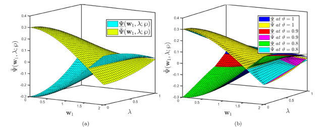
Fig. 4.9. Solution profiles of Problem 4.3 demonstrate (a) Lower and upper case solutions for (b) Lower and upper case solutions for |
Fig. 4.10 displays the analysis of Problem 4.3 under -differentiabilty of CFD (a) the two dimensional approximate solution with various fractional orders but fixed uncertain parameters (b) the two dimensional approximate solution with various uncertain parameters but fixed fractional order .

Fig. 4.10. (a) Solution profiles by Caputo fractional derivative of Problem 4.3 demonstrate (a) Lower and upper case solutions for different fractional orders with uncertainty parameter and λ=0.5. (b) Lower and upper case solutions for various uncertainties with and λ=0.5. |
Fig. 4.11 illustrates the analysis of Problem 4.3 under -differentiabilty of ABC fractional derivative (a) the two dimensional approximate solution with various fractional orders but fixed uncertain parameter (b) the two dimensional approximate solution with various uncertain parameters but fixed fractional order .
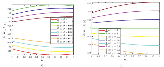
Fig. 4.11. Solution profiles by ABC fractional derivative of Problem 4.3 demonstrate (a) Lower and upper case solutions for different fractional orders with uncertainty parameter and λ=0.5. (b) Lower and upper case solutions for various uncertainties with and λ=0.5. |
Fig. 4.12 defines the comparison analysis of Problem 4.3 under -differentiabilty of Caputo and ABC fractional derivatives (a) 3D simulation (b) 2D simulation.
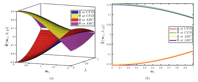
Fig. 4.12. Comparisons solution profiles by Caputo and ABC fractional derivative of Problem 4.1 demonstrates (a) three dimensional lower and upper case solutions, (b) two dimensional lower and upper case solutions, when and λ=0.5. |
At the third term approximation, the values of the numerical results of multiple grid points generated by the GHPTM are comparable to the values of the exact solution with high accuracy, indicating a high level of conformity with the two findings of different fractional operators with excellent convergence between them. Furthermore, by implementing inferential statistical testing, the proposed method will aid scientists working on magneto-acoustic waves occurring in plasma and fullid mechanics in assessing competency.
Remark 4.3. Letting $ \underline{\Upsilon}(\wp)=\bar{\Upsilon}(\wp)=1$, then the approximate solution of Problem 4.3 reduces to
Problem 4.4. Consider the fuzzy fractional dispersive KdV model:
$ \frac{\partial^{\vartheta}}{\partial \lambda^{\vartheta}} \widetilde{\Psi}\left(\mathbf{w}_{1}, \mathbf{w}_{2}, \lambda ; \wp\right)=\ominus \frac{\partial^{3}}{\partial \mathbf{w}_{1}^{3}} \widetilde{\Psi}\left(\mathbf{w}_{1}, \mathbf{w}_{2}, \lambda ; \wp\right) \ominus \frac{\partial^{3}}{\partial \mathbf{w}_{2}^{3}} \widetilde{\Psi}\left(\mathbf{w}_{1}, \mathbf{w}_{2}, \lambda ; \wp\right) $
subject to fuzzy ICs
$ \widetilde{\Psi}\left(\mathbf{w}_{1}, \mathbf{w}_{2}, 0\right)=\widetilde{\Upsilon}(\wp) \odot \cos \left(\mathbf{w}_{1}+\mathbf{w}_{2}\right), $
where $ \widetilde{\Upsilon}(\wp)=[\underline{\Upsilon}(\wp), \bar{\Upsilon}(\wp)]=[\wp-1,1-\wp]$ for is fuzzy number.
The parameterized formulation of (4.14) is presented as
$ \left\{\begin{array}{l} \frac{\partial^{\vartheta}}{\partial \lambda^{\vartheta}} \Psi\left(\mathbf{w}_{1}, \mathbf{w}_{2}, \lambda ; \wp\right)=-\frac{\partial^{3}}{\partial \mathbf{w}_{1}^{3}} \Psi\left(\mathbf{w}_{1}, \mathbf{w}_{2}, \lambda ; \wp\right)-\frac{\partial^{3}}{\partial \mathbf{w}_{2}^{3}} \underline{\Psi}\left(\mathbf{w}_{1}, \mathbf{w}_{2}, \lambda ; \wp\right), \\ \underline{\Psi}\left(\mathbf{w}_{1}, \mathbf{w}_{2}, 0\right)=(\wp-1) \cos \left(\mathbf{w}_{1}+\mathbf{w}_{2}\right) \\ \frac{\partial^{\vartheta}}{\partial \lambda^{\vartheta}} \Psi\left(\mathbf{w}_{1}, \mathbf{w}_{2}, \lambda ; \wp\right)=-\frac{\partial^{3}}{\partial \mathbf{w}_{1}^{3}} \Psi\left(\mathbf{w}_{1}, \mathbf{w}_{2}, \lambda ; \wp\right)-\frac{\partial^{3}}{\partial \mathbf{w}_{2}^{3}} \Psi\left(\mathbf{w}_{1}, \mathbf{w}_{2}, \lambda ; \wp\right), \\ \bar{\Psi}\left(\mathbf{w}_{1}, \mathbf{w}_{2}, 0\right)=(1-\wp) \cos \left(\mathbf{w}_{1}+\mathbf{w}_{2}\right). \end{array}\right. $
Case I. Firstly, taking into consideration the CFD coupled with the generalized homotopy perturbation transform method on the first case of (4.3).
In view of the process stated in Section 3, we have
$\begin{array}{l} \Phi^{\vartheta}\left(s_{1}\right) \mathbf{J}\left[\underline{\Psi}\left(\mathbf{w}_{1}, \lambda ; \wp\right)\right]-\Theta\left(s_{1}\right) \sum_{\kappa=0}^{q-1} \Phi^{\vartheta-1-\kappa}\left(s_{1}\right) \underline{\Psi}^{(\kappa)}\left(\mathbf{w}_{1}, 0 ; \wp\right) \\ =\mathbf{J}\left[-\frac{\partial^{3}}{\partial \mathbf{w}_{1}^{3}} \underline{\Psi}\left(\mathbf{w}_{1}, \mathbf{w}_{2}, \lambda ; \wp\right)-\frac{\partial^{3}}{\partial \mathbf{w}_{2}^{3}} \underline{\Psi}\left(\mathbf{w}_{1}, \mathbf{w}_{2}, \lambda ; \wp\right)\right]. \end{array}$
In view of fuzzy IC and making use of the inverse generalized integral transform implies
$\begin{array}{l} \underline{\Psi}\left(\mathbf{w}_{1}, \mathbf{w}_{2}, \lambda ; \wp\right)=(\wp-1) \cos \left(\mathbf{w}_{1}+\mathbf{w}_{2}\right)+\mathbf{J}^{-1}\left[\frac { 1 } { \Phi ^ { \vartheta } ( s _ { 1 } ) } \mathbf { J } \left[-\frac{\partial^{3}}{\partial \mathbf{w}_{1}^{3}} \underline{\Psi}\left(\mathbf{w}_{1}, \mathbf{w}_{2}, \lambda ; \wp\right)\right.\right. \\ \left.\left.-\frac{\partial^{3}}{\partial \mathbf{w}_{2}^{3}} \underline{\Psi}\left(\mathbf{w}_{1}, \mathbf{w}_{2}, \lambda ; \wp\right)\right]\right] \end{array}$
Now implementing the HPM, we have
$\begin{aligned} \sum_{\kappa=0}^{\infty} \eta^{\kappa} \underline{\Psi}_{\kappa}\left(\mathbf{w}_{1}, \mathbf{w}_{2}, \lambda ; \wp\right)= & (\wp-1) \cos \left(\mathbf{w}_{1}+\mathbf{w}_{2}\right) \\ & -\eta\left(\mathbf{J}^{-1}\left[\frac{1}{\Phi^{\vartheta}\left(s_{1}\right)} \mathbf{J}\left[\left(\sum_{\kappa=0}^{\infty} \eta^{\kappa} \underline{\Psi}_{\kappa}\left(\mathbf{w}_{1}, \lambda ; \wp\right)\right) 3 \mathbf{w}_{1}+\left(\sum_{\kappa=0}^{\infty} \eta^{\kappa} \underline{\Psi}_{\kappa}\left(\mathbf{w}_{1}, \lambda ; \wp\right)\right) 3 \mathbf{w}_{2}\right]\right]\right). \end{aligned}$
Equating the coefficients of the same powers of η, we have
$\begin{aligned} \eta^{0}: \underline{\Psi}_{0}\left(\mathbf{w}_{1}, \mathbf{w}_{2}, \lambda ; \wp\right) & =(\wp-1) \cos \left(\mathbf{w}_{1}+\mathbf{w}_{2}\right) \\ \eta^{1}: \underline{\Psi}_{1}\left(\mathbf{w}_{1}, \mathbf{w}_{2}, \lambda ; \wp\right) & =-\mathbf{J}^{-1}\left[\frac{1}{\Phi^{\vartheta}\left(s_{1}\right)} \mathbf{J}\left[\left(\underline{\Psi}_{0}\left(\mathbf{w}_{1}, \mathbf{w}_{2}, \lambda ; \wp\right)\right) 3 \mathbf{w}_{1}+\left(\underline{\Psi}_{0}\left(\mathbf{w}_{1}, \mathbf{w}_{2}, \lambda ; \wp\right)\right) 3 \mathbf{w}_{2}\right]\right] \\ & =-2(\wp-1) \sin \left(\mathbf{w}_{1}+\mathbf{w}_{2}\right) \frac{\lambda^{\vartheta}}{\Gamma(\vartheta+1)}, \\ \eta^{2}: \underline{\Psi}_{2}\left(\mathbf{w}_{1}, \mathbf{w}_{2}, \lambda ; \wp\right) & =-\mathbf{J}^{-1}\left[\frac{1}{\Phi^{\vartheta}\left(s_{1}\right)} \mathbf{J}\left[\left(\underline{\Psi}_{1}\left(\mathbf{w}_{1}, \mathbf{w}_{2}, \lambda ; \wp\right)\right) 3 \mathbf{w}_{1}+2\left(\underline{\Psi}_{1}\left(\mathbf{w}_{1}, \mathbf{w}_{2}, \lambda ; \wp\right)\right) 3 \mathbf{w}_{2}\right]\right] \\ & =-4(\wp-1) \cos \left(\mathbf{w}_{1}+\mathbf{w}_{2}\right) \frac{\lambda^{2 \vartheta}}{\Gamma(2 \vartheta+1)}, \\ \eta^{3}: \underline{\Psi}_{3}\left(\mathbf{w}_{1}, \mathbf{w}_{2}, \lambda ; \wp\right) & =-\mathbf{J}^{-1}\left[\frac{1}{\Phi^{\vartheta}\left(s_{1}\right)} \mathbf{J}\left[\left(\underline{\Psi}_{2}\left(\mathbf{w}_{1}, \mathbf{w}_{2}, \lambda ; \wp\right)\right) 3 \mathbf{w}_{1}+2\left(\underline{\Psi}_{2}\left(\mathbf{w}_{1}, \mathbf{w}_{2}, \lambda ; \wp\right)\right) 3 \mathbf{w}_{2}\right]\right] \\ & =8(\wp-1) \sin \left(\mathbf{w}_{1}+\mathbf{w}_{2}\right) \frac{\lambda^{3 \vartheta}}{\Gamma(3 \vartheta+1)}, \\ \vdots. & \end{aligned}$
The series form solution is presented as follows
$\begin{array}{l} \widetilde{\Psi}\left(\mathbf{w}_{1}, \mathbf{w}_{2}, \lambda ; \wp\right)=\widetilde{\Psi}_{0}\left(\mathbf{w}_{1}, \mathbf{w}_{2}, \lambda ; \wp\right)+\widetilde{\Psi}_{1}\left(\mathbf{w}_{1}, \mathbf{w}_{2}, \lambda ; \wp\right)+\widetilde{\Psi}_{2}\left(\mathbf{w}_{1}, \mathbf{w}_{2}, \lambda ; \wp\right) \\ +\widetilde{\Psi}_{3}\left(\mathbf{w}_{1}, \mathbf{w}_{2}, \lambda ; \wp\right)+\ldots, \end{array}$
implies that
$\begin{aligned} \underline{\Psi}\left(\mathbf{w}_{1}, \mathbf{w}_{2}, \lambda ; \wp\right) & =\Psi_{0}\left(\mathbf{w}_{1}, \mathbf{w}_{2}, \lambda ; \wp\right)+\underline{\Psi}_{1}\left(\mathbf{w}_{1}, \mathbf{w}_{2}, \lambda ; \wp\right)+\underline{\Psi}_{2}\left(\mathbf{w}_{1}, \mathbf{w}_{2}, \lambda ; \wp\right)+\underline{\Psi}_{3}\left(\mathbf{w}_{1}, \mathbf{w}_{2}, \lambda ; \wp\right) \\ & +\ldots, \\ \bar{\Psi}\left(\mathbf{w}_{1}, \mathbf{w}_{2}, \lambda ; \wp\right) & =\bar{\Psi}_{0}\left(\mathbf{w}_{1}, \mathbf{w}_{2}, \lambda ; \wp\right)+\bar{\Psi}_{1}\left(\mathbf{w}_{1}, \mathbf{w}_{2}, \lambda ; \wp\right)+\bar{\Psi}_{2}\left(\mathbf{w}_{1}, \mathbf{w}_{2}, \lambda ; \wp\right)+\bar{\Psi}_{3}\left(\mathbf{w}_{1}, \mathbf{w}_{2}, \lambda ; \wp\right) \\ & +\ldots \end{aligned}$
Finally, we have
$\begin{aligned} \underline{\Psi}\left(\mathbf{w}_{1}, \mathbf{w}_{2}, \lambda ; \wp\right)= & (\wp-1) \cos \left(\mathbf{w}_{1}+\mathbf{w}_{2}\right)\left[1-\frac{4 \lambda^{2 \vartheta}}{\Gamma(2 \vartheta+1)}+\frac{16 \lambda^{4 \vartheta}}{\Gamma(4 \vartheta+1)}-\ldots\right] \\ & +(\wp-1) \sin \left(\mathbf{w}_{1}+\mathbf{w}_{2}\right)\left[\frac{2 \lambda^{\vartheta}}{\Gamma(\vartheta+1)}-\frac{8 \lambda^{3 \vartheta}}{\Gamma(3 \vartheta+1)}+\frac{32 \lambda^{5 \vartheta}}{\Gamma(5 \vartheta+1)}-\ldots\right] \\ \bar{\Psi}\left(\mathbf{w}_{1}, \mathbf{w}_{2}, \lambda ; \wp\right)= & (1-\wp) \cos \left(\mathbf{w}_{1}+\mathbf{w}_{2}\right)\left[1-\frac{4 \lambda^{2 \vartheta}}{\Gamma(2 \vartheta+1)}+\frac{16 \lambda^{4 \vartheta}}{\Gamma(4 \vartheta+1)}-\ldots\right] \\ & +(1-\wp) \sin \left(\mathbf{w}_{1}+\mathbf{w}_{2}\right)\left[\frac{2 \lambda^{\vartheta}}{\Gamma(\vartheta+1)}-\frac{8 \lambda^{3 \vartheta}}{\Gamma(3 \vartheta+1)}+\frac{32 \lambda^{5 \vartheta}}{\Gamma(5 \vartheta+1)}-\ldots\right] \end{aligned}$
Case 2. Now, we employ the fuzzy ABC derivative operator on the first first case of (4.3) as follows:
In view of the process stated in Section 3, we have
$\begin{aligned} & \frac{\Phi^{\vartheta}\left(s_{1}\right) \mathbb{B}(\vartheta)}{\vartheta+(1-\vartheta) \Phi^{\vartheta}(s)}\left[\underline{\mathscr{U}}\left(\mathbf{w}_{1}, s_{1} ; \wp\right)-\frac{\Theta\left(s_{1}\right)}{\Phi(s)} \underline{\Psi}\left(\mathbf{w}_{1}, 0 ; \wp\right)\right] \\ = & \mathbf{J}\left[\left[-\frac{\partial^{3}}{\partial \mathbf{w}_{1}^{3}} \underline{\Psi}\left(\mathbf{w}_{1}, \mathbf{w}_{2}, \lambda ; \wp\right)-\frac{\partial^{3}}{\partial \mathbf{w}_{2}^{3}} \underline{\Psi}\left(\mathbf{w}_{1}, \mathbf{w}_{2}, \lambda ; \wp\right)\right].\right. \end{aligned}$
In view of fuzzy IC and making use of the inverse generalized integral transform implies
$\begin{aligned} \underline{\Psi}\left(\mathbf{w}_{1}, \mathbf{w}_{2}, \lambda ; \wp\right) & =(\wp-1) \cos \left(\mathbf{w}_{1}+\mathbf{w}_{2}\right) \\ & +\mathbf{J}^{-1}\left[\frac{\vartheta+(1-\vartheta) \Phi^{\vartheta}(s)}{\Phi^{\vartheta}\left(s_{1}\right) \mathbb{B}(\vartheta)} \mathbf{J}\left[\left[-\frac{\partial^{3}}{\partial \mathbf{w}_{1}^{3}} \underline{\Psi}\left(\mathbf{w}_{1}, \mathbf{w}_{2}, \lambda ; \wp\right)-\frac{\partial^{3}}{\partial \mathbf{w}_{2}^{3}} \underline{\Psi}\left(\mathbf{w}_{1}, \mathbf{w}_{2}, \lambda ; \wp\right)\right]\right].\right. \end{aligned}$
Now implementing the HPM, we have
$\begin{aligned} \sum_{\kappa=0}^{\infty} \quad & \eta^{\kappa} \underline{\Psi}_{\kappa}\left(\mathbf{w}_{1}, \mathbf{w}_{2}, \lambda ; \wp\right)=(\wp-1) \cos \left(\mathbf{w}_{1}+\mathbf{w}_{2}\right) \\ & -\eta\left(\mathbf { J } ^ { - 1 } \left[\frac { \vartheta + ( 1 - \vartheta ) \Phi ^ { \vartheta } ( s ) } { \Phi ^ { \vartheta } ( s _ { 1 } ) \mathbb { B } ( \vartheta ) } \mathbf { J } \left[\left(\sum_{\kappa=0}^{\infty} \eta^{\kappa} \underline{\Psi}_{\kappa}\left(\mathbf{w}_{1}, \lambda ; \wp\right)\right) 3 \mathbf{w}_{1}\right.\right.\right. \\ & \left.\left.\left.+\left(\sum_{\kappa=0}^{\infty} \eta^{\kappa} \underline{\Psi}_{\kappa}\left(\mathbf{w}_{1}, \lambda ; \wp\right)\right) 3 \mathbf{w}_{2}\right]\right]\right). \end{aligned}$
Equating the coefficients of the same powers of η, we have
$\begin{aligned} \eta^{0}: \underline{\Psi}_{0}\left(\mathbf{w}_{1}, \mathbf{w}_{2}, \lambda ; \wp\right) & =(\wp-1) \cos \left(\mathbf{w}_{11}+\mathbf{w}_{2}\right), \\ \eta^{1}: \underline{\Psi}_{1}\left(\mathbf{w}_{1}, \mathbf{w}_{2}, \lambda ; \wp\right) & =-\mathbf{J}^{-1}\left[\frac { \vartheta + ( 1 - \vartheta ) \Phi ^ { \vartheta } ( s ) } { \Phi ^ { \vartheta } ( s _ { 1 } ) \mathbb { B } ( \vartheta ) } \mathbf { J } \left[\left(\underline{\Psi}_{0}\left(\mathbf{w}_{1}, \mathbf{w}_{2}, \lambda ; \wp\right)\right) 3 \mathbf{w}_{1}\right.\right. \\ & \left.\left.+\left(\underline{\Psi}_{0}\left(\mathbf{w}_{1}, \mathbf{w}_{2}, \lambda ; \wp\right)\right) 3 \mathbf{w}_{2}\right]\right] \\ & =-2(\wp-1) \sin \left(\mathbf{w}_{1}+\mathbf{w}_{2}\right)\left(\frac{\vartheta \lambda^{\vartheta}}{\Gamma(\vartheta+1)}+(1-\vartheta)\right), \\ \eta^{2}: \underline{\Psi}_{2}\left(\mathbf{w}_{1}, \mathbf{w}_{2}, \lambda ; \wp\right)= & -\mathbf{J}^{-1}\left[\frac { \vartheta + ( 1 - \vartheta ) \Phi ^ { \vartheta } ( s ) } { \Phi ^ { \vartheta } ( s _ { 1 } ) \mathbb { B } ( \vartheta ) } \mathbf { J } \left[\left(\underline{\Psi}_{1}\left(\mathbf{w}_{1}, \mathbf{w}_{2}, \lambda ; \wp\right)\right) 3 \mathbf{w}_{1}\right.\right. \\ & \left.\left.+\left(\underline{\Psi}_{1}\left(\mathbf{w}_{1}, \mathbf{w}_{2}, \lambda ; \wp\right)\right) 3 \mathbf{w}_{2}\right]\right] \\ = & -4(\wp-1) \cos \left(\mathbf{w}_{1}+\mathbf{w}_{2}\right)\left(\frac{\vartheta^{2} \lambda^{2 \vartheta}}{\Gamma(2 \vartheta+1)}+2 \vartheta(1-\vartheta) \frac{\lambda^{\vartheta}}{\Gamma(\vartheta+1)}+(1-\vartheta)^{2}\right), \\ \eta^{3}: \underline{\Psi}_{2}\left(\mathbf{w}_{1}, \mathbf{w}_{2}, \lambda ; \wp\right) & -\mathbf{J}^{-1}\left[\frac { \vartheta + ( 1 - \vartheta ) \Phi ^ { \vartheta } ( s ) } { \Phi ^ { \vartheta } ( s _ { 1 } ) \mathbb { B } ( \vartheta ) } \mathbf { J } \left[\left(\underline{\Psi}_{2}\left(\mathbf{w}_{1}, \mathbf{w}_{2}, \lambda ; \wp\right)\right) 3 \mathbf{w}_{1}\right.\right. \\ & \left.\left.+\left(\underline{\Psi}_{2}\left(\mathbf{w}_{1}, \mathbf{w}_{2}, \lambda ; \wp\right)\right) 3 \mathbf{w}_{2}\right]\right] \\ = & 8(\wp-1) \sin \left(\mathbf{w}_{1}+\mathbf{w}_{2}\right)\left(\frac{\vartheta^{3} \lambda^{3 \vartheta}}{\Gamma(3 \vartheta+1)}+3 \vartheta^{2}(1-\vartheta) \frac{\lambda^{2 \vartheta}}{\Gamma(2 \vartheta+1)}\right. \\ & \left.+3 \vartheta(1-\vartheta)^{2} \frac{\lambda^{\vartheta}}{\Gamma(\vartheta+1)}+(1-\vartheta)^{3}\right), \\ \vdots. & \end{aligned}$
The series form solution is presented as follows:
$\begin{array}{l} \widetilde{\Psi}\left(\mathbf{w}_{1}, \mathbf{w}_{2}, \lambda ; \wp\right)=\widetilde{\Psi}_{0}\left(\mathbf{w}_{1}, \mathbf{w}_{2}, \lambda ; \wp\right)+\widetilde{\Psi}_{1}\left(\mathbf{w}_{1}, \mathbf{w}_{2}, \lambda ; \wp\right)+\widetilde{\Psi}_{2}\left(\mathbf{w}_{1}, \mathbf{w}_{2}, \lambda ; \wp\right) \\ +\widetilde{\Psi}_{3}\left(\mathbf{w}_{1}, \mathbf{w}_{2}, \lambda ; \wp\right)+\ldots ; \end{array}$
implies that
$\begin{aligned} \underline{\Psi}\left(\mathbf{w}_{1}, \mathbf{w}_{2}, \lambda ; \wp\right) & =\underline{\Psi}_{0}\left(\mathbf{w}_{1}, \mathbf{w}_{2}, \lambda ; \wp\right)+\underline{\Psi}_{1}\left(\mathbf{w}_{1}, \mathbf{w}_{2}, \lambda ; \wp\right)+\underline{\Psi}_{2}\left(\mathbf{w}_{1}, \mathbf{w}_{2}, \lambda ; \wp\right)+\underline{\Psi}_{3}\left(\mathbf{w}_{1}, \mathbf{w}_{2}, \lambda ; \wp\right) \\ & +\ldots, \\ \bar{\Psi}\left(\mathbf{w}_{1}, \mathbf{w}_{2}, \lambda ; \wp\right) & =\bar{\Psi}_{0}\left(\mathbf{w}_{1}, \mathbf{w}_{2}, \lambda ; \wp\right)+\bar{\Psi}_{1}\left(\mathbf{w}_{1}, \mathbf{w}_{2}, \lambda ; \wp\right)+\bar{\Psi}_{2}\left(\mathbf{w}_{1}, \mathbf{w}_{2}, \lambda ; \wp\right)+\bar{\Psi}_{3}\left(\mathbf{w}_{1}, \mathbf{w}_{2}, \lambda ; \wp\right) \\ & +\ldots \end{aligned}$
Finally, we have
$\begin{array}{l} \underline{\Psi}\left(\mathbf{w}_{1}, \mathbf{w}_{2}, \lambda ; \wp\right)=(\wp-1) \cos \left(\mathbf{w}_{1}+\mathbf{w}_{2}\right)\left[1-4\left(\frac{\vartheta^{2} \lambda^{2 \vartheta}}{\Gamma(2 \vartheta+1)}+2 \vartheta(1-\vartheta) \frac{\lambda^{\vartheta}}{\Gamma(\vartheta+1)}\right.\right. \\ \left.+(1-\vartheta)^{2}\right) \\ \quad+16\left(\frac{\vartheta^{4} \lambda^{4 \vartheta}}{\Gamma(4 \vartheta+1)}+4 \vartheta^{3}(1-\vartheta) \frac{\lambda^{3 \vartheta}}{\Gamma(3 \vartheta+1)}+6 \vartheta^{2}(1-\vartheta)^{2} \frac{\lambda^{2 \vartheta}}{\Gamma(2 \vartheta+1)}\right. \\ \left.\left.+4 \vartheta(1-\vartheta)^{3} \frac{\lambda^{\vartheta}}{\Gamma(\vartheta+1)}+(1-\vartheta)^{4}\right)-\ldots\right] \\ \quad+(\wp-1) \sin \left(\mathbf{w}_{1}+\mathbf{w}_{2}\right)\left[2\left(\frac{\vartheta \lambda^{\vartheta}}{\Gamma(\vartheta+1)}+(1-\vartheta)\right)\right. \\ -8\left(\frac{\vartheta^{3} \lambda^{3 \vartheta}}{\Gamma(3 \vartheta+1)}+3 \vartheta^{2}(1-\vartheta) \frac{\lambda^{2 \vartheta}}{\Gamma(2 \vartheta+1)}+3 \vartheta(1-\vartheta)^{2} \frac{\lambda^{\vartheta}}{\Gamma(\vartheta+1)}\right. \\ \left.\left.+(1-\vartheta)^{3}\right)+\ldots\right], \end{array}$
$\begin{array}{l} \bar{\Psi}\left(\mathbf{w}_{1}, \mathbf{w}_{2}, \lambda ; \wp\right)=(1-\wp) \cos \left(\mathbf{w}_{1}+\mathbf{w}_{2}\right)\left[1-4\left(\frac{\vartheta^{2} \lambda^{2 \vartheta}}{\Gamma(2 \vartheta+1)}+2 \vartheta(1-\vartheta) \frac{\lambda^{\vartheta}}{\Gamma(\vartheta+1)}\right.\right. \\ \left.+(1-\vartheta)^{2}\right) \\ \quad+16\left(\frac{\vartheta^{4} \lambda^{4 \vartheta}}{\Gamma(4 \vartheta+1)}+4 \vartheta^{3}(1-\vartheta) \frac{\lambda^{3 \vartheta}}{\Gamma(3 \vartheta+1)}+6 \vartheta^{2}(1-\vartheta)^{2} \frac{\lambda^{2 \vartheta}}{\Gamma(2 \vartheta+1)}\right. \\ \left.\left.+4 \vartheta(1-\vartheta)^{3} \frac{\lambda^{\vartheta}}{\Gamma(\vartheta+1)}+(1-\vartheta)^{4}\right)-\ldots\right] \\ \quad+(1-\wp) \sin \left(\mathbf{w}_{1}+\mathbf{w}_{2}\right)\left[2\left(\frac{\vartheta \lambda^{\vartheta}}{\Gamma(\vartheta+1)}+(1-\vartheta)\right)\right. \\ -8\left(\frac{\vartheta^{3} \lambda^{3 \vartheta}}{\Gamma(3 \vartheta+1)}+3 \vartheta^{2}(1-\vartheta) \frac{\lambda^{2 \vartheta}}{\Gamma(2 \vartheta+1)}+3 \vartheta(1-\vartheta)^{2} \frac{\lambda^{\vartheta}}{\Gamma(\vartheta+1)}\right. \\ \left.\left.+(1-\vartheta)^{3}\right)+\ldots\right], \end{array}$
From Fig. 4.13 represents the analysis of Problem 4.4 (a) the lower and upper accuracy for the approximate solutions under -differentiabilty of CFD when (b) the lower and upper accuracy for the approximate solutions under -differentiabilty of CFD when It is worth mentioning that as the accuracies increase, the order of approximations increases. Fig. 4.14 displays the analysis of Problem 4.4 under -differentiabilty of CFD (a) the two dimensional approximate solution with various fractional orders but fixed uncertain parameters (b) the two dimensional approximate solution with various uncertain parameters but fixed fractional order .

Fig. 4.13. Solution profiles of Problem 4.1 demonstrate (a) Lower and upper case solutions for (b) Lower and upper case solutions for , and 0.8. |
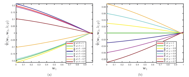
Fig. 4.14. Solution profiles by Caputo fractional derivative of Problem 4.4 demonstrate (a) Lower and upper case solutions for different fractional orders with uncertainty parameter and λ=0.5. (b) Lower and upper case solutions for various uncertainties with and λ=0.5. |
Fig. 4.15 illustrates the analysis of Problem 4.4 under -differentiabilty of ABC fractional derivative (a) the two dimensional approximate solution with various fractional orders but fixed uncertain parameter (b) the two dimensional approximate solution with various uncertain parameters but fixed fractional order .
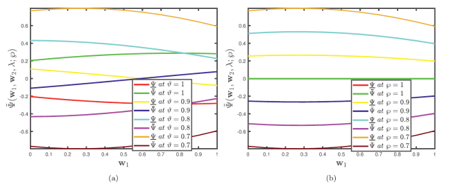
Fig. 4.15. Solution profiles by ABC fractional derivative of Problem 4.4 demonstrate (a) Lower and upper case solutions for different fractional orders with uncertainty parameter and λ=0.5. (b) Lower and upper case solutions for various uncertainties with and λ=0.5. |
Fig. 4.16 defines the comparison analysis of Problem 4.4 under -differentiabilty of Caputo and ABC fractional derivatives (a) 3D simulation (b) 2D simulation.
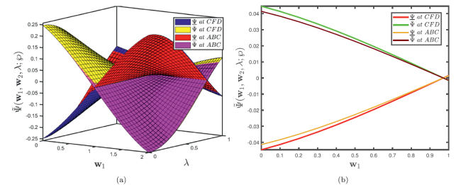
Fig. 4.16. Comparisons solution profiles by Caputo and ABC fractional derivative of Problem 4.1 demonstrates (a) three dimensional lower and upper case solutions, (b) two dimensional lower and upper case solutions, when ℘=.7,ϑ=1 and λ=0.5. |
At the third term approximation, the values of the numerical results of multiple grid points generated by the GHPTM are comparable to the values of the exact solution with high accuracy, indicating a high level of conformity with the two findings of different fractional operators with excellent convergence between them. Furthermore, by implementing inferential statistical testing, the proposed method will aid scientists working on magneto-acoustic waves occurring in plasma and fullid mechanics in assessing competency.
Remark 4.4. Letting $\Upsilon(\wp)=\bar{\Upsilon}(\wp)=1$, then the approximate solution of Problem 4.4 reduces to $\Psi\left(\mathbf{w}_{1}, \lambda\right)=\cos \left(\mathbf{w}_{1}+\mathbf{w}_{2}+2 \lambda\right)$.
5. Conclusion
We have successfully combined the generalized integral transform with a HPTM in a limited setting for the approximation of nonlinear dispersive and fifth order KdV models with the CFD and ABC fractional derivatives under gH differentiability in this investigation. The generalized integral transform transform simplified the problem to a time independent problem, alleviating the necessity for the traditional time stepping approach. For various fractional orders and uncertainty ℘∈[0,1], numerical tests were conducted for KdV equations with a CFD and ABC fractional derivative. Furthermore, 2D and 3D simulations have been carried out and comparison graphs are presented that demonstrate the effectiveness and supremacy of the proposed method. From the findings, we can deduce that GHPTM is reliable in approximating the phenomenon of atmospheric internal waves. The proposed findings provide a thorough and pragmatic look into the behaviour of these waves, which can be leveraged to refine weather and climate models, as the waves have a significant influence on climate change as well as beachfront ocean and ocean engineering, as has been observed in recent years.
Declarations
Availability of supporting data Not applicable. Competing interests The authors declare that they have no competing interests. Funding Not Applicable Author’s contributions All authors contributed equally to the writing of this paper. All authors read and approved the nal manuscript.
Declaration of Competing Interest
The authors declare no conflict of interest.
