
1. Introduction
Many researchers investigated the Nonlinear propagating dust-acoustic solitary waves (DASWs) in a heated magnetized dusty plasma containing various sizes and mass negatively charged dust particles, isothermal electrons, high- and low-temperature ions. The Zakharov-Kuznetsov equation for the first-order perturbed potential was obtained using an adequate normalization of the hydrodynamic and Poisson equations. As the wave amplitude rose, the width and velocity of the solitons deviated from the predictions of the Zakharov-Kuznetsov equations. A linear inhomogeneous type Zakharov-Kuznetsov equation for the second-order perturbed potential was devised to explain the soliton of higher amplitude, whereas the re normalization method was used to provide stationary solutions to both equations. For the study of vortices in geophysical flows, The Zakharov-Kuznetsov equation was a beneficial model equation. The ZK equation, the electrostatic-acoustic pulses are analyzed in magnetized ions, is one of the notorious variations of the Korteweg-de Vries equations. The ZK equations are the investigation of coastal waves on the bases of ocean [1], [2], [3], [4]. ZK equation was initially introduced while studying weak nonlinear acoustic ion waves, which attract losses of two-dimensional ions. In the current work, we look at the following fractional-order ZK equation:
$D_{t}^{\alpha} v+C_{1}\left(v^{a_{1}}\right)_{x}+C_{2}\left(v^{a_{2}}\right)_{x x x}+C_{3}\left(v^{a_{3}}\right)_{x y y}=0$
where, , α∈(0,1] is parameter which defines the fractional order structure and are arbitrary constants [5]. are integers and because of ai, the construction of weak nonlinear acoustic ion vibrations in a plasma comprising cooling,hot exothermic electrons in the systematic electric field is possible [6].
Leibniz first mentioned the name of fractional calculus; the well-known German mathematician sent a letter to other well-known mathematicians from France named L’Hopital in the last decade of the 17th century. In the research article, fractional calculus was first introduced by Abel [7]. Throughout time other great mathematicians Liouville [8], [9], Reimann [10], Caputo [11] and many others [12], [13], [14], [15], [16] contributed their huge knowledge about the field. Fractional calculus has always been getting lots of attention by researchers due to its application in real-world physics problems and almost every engineering branch. There are many approaches available for the solution of nonlinear and fractional order differential equations [17], [18], [19], [20]. The solution of Fractional order ZK equation(FZK) was illustrated by many techniques as fractional iteration method (FIM) [21], perturbation-iteration algorithm and continues power series technique [6], New iterative Sumudu transform method(NISTM) [22], variational iteration method(VIM) [23], homotopy perturbation transform method(HPTM) [5], Laplace Adomian decomposition method(LADM) [24], fractional natural decomposition method(FNDM) and q-homotopy analysis transform method(q-HATM) [5], optimum homotopy asymptotic method(OHAM) [26], Homotopy analysis fractional Sumudu transform method(HAFSTM) [27], natural transform decomposition method(NTDM) [29] and Elzaki transform iterative method(ETIM) [28]. All these techniques are providing an approximate solution for fractional nonlinear problem. The homotopy analysis method (HAM) was first introduced by Liao [30], [31], [32] in 1992 with the application of fundamental differentiation and geometry concept i.e. called homotopy. HAM was very beneficial for finding solution of many linear, nonlinear and fractional differential equation based problems [33], [34], [35], [36], [37], [38], [39], [40], [41]. HAM was handy to find the solution without using perturbations or linearisation, and the method required a lot of computational work and a faster computer. To overcome these limitations, in 2012, El-Tawil and Huseen proposed a modified technique of HAM called q-Homotopy Analysis Method(q-HAM) [42], [43]. q-HAM introduced a parameter to control the convergence of series solution. As it was complex to find a solution of fractional order differential equation using, Singh et al. [44] introduced a new technique called q-HATM, which was a combination of q-HAM and Laplace transform in 2016. Next year, Singh et al. [45] used Sumudu transform instead of Laplace transform and provided a new approach to called q-homotopy analysis Sumudu transform method(q-HASTM). Jena and Chakraverty [46] came up with the combination of q-HAM and Aboodh transform and introduced a method called q-homotopy analysis Aboodh transform method(q-HAATM) in 2019. In 2021, q-homotopy analysis Elzaki transform method(q-HAETM) was introduced by Singh et al. [47]. As all those transforms have some limitations and not having direct use to many mathematical and nonlinear problems, it was not directly applicable to some problems. In 2019, Maitama and Zhao [48], introduced a new transform called Shehu transform to overcome limitations of available integral transforms. Later, Maitama and Zhao applied the Shehu transform successfully with the Homotopy Analysis Method to solve multidimensional fractional diffusion equation [49]. In this paper, we introduce the new homotopy technique called q-homotopy analysis Shehu transform method(q-HAShTM), a combination of the q-Homotopy analysis method and Shehu transform. This method controls the convergence of the series solution because of two parameters n and . The proposed technique is a time-saving technique and less complex than other techniques, and the efficiency is better.
2. Preliminaries
${ }^{R L} \mathbb{D}_{t}^{\alpha} g(t)=\frac{1}{\Gamma(n-\alpha)} \frac{d^{n}}{d t^{n}} \int_{0}^{t}(t-\varsigma)^{n-\alpha-1} g(\varsigma) d \varsigma$
$\mathfrak{I}^{\alpha} g(t)=\left\{\begin{array}{ll} \frac{1}{\Gamma(\alpha)} \int_{0}^{t}(t-\mu)^{\alpha-1} g(\mu) d \mu, & \alpha>0, t>0 \\ g(t), & \alpha=0 . \end{array}\right.$
Definition 2.4 The derivative of with fractional order in the sense of Caputo [16] is defined as
$ \mathbb{D}_{t}^{\alpha} g(t)=\left\{\begin{array}{ll} \frac{1}{\Gamma(n-\alpha)} \int_{0}^{t}(t-\mu)^{n-\alpha-1} g^{n}(\mu) d \mu, & n-1<\alpha<n, n \in \mathbb{N} \\ \mathfrak{I}^{n-\alpha} \mathbb{D}^{n} g(t) & \alpha=n \in \mathbb{N}. \end{array}\right. $
Definition 2.5 The Shehu transform [48] of the function with
$\begin{array}{l} A=\left\{g(t)\left|\exists K, \kappa_{1}, \kappa_{2}>0,\right| g(t) \left\lvert\,<K \exp \left(\frac{|t|}{\kappa_{i}}\right)\right.,\right. \\ \left.\quad \text { if } t \in(-1)^{i} \times[0, \infty)\right\}, \end{array}$
is defined by
$ G(s, u)=\mathscr{S}[g(t)]=\int_{0}^{\infty} \exp \left(\frac{-s t}{u}\right) g(t) d t. $
where, s and u are positive numbers. Here, we can conduct the following results using Eq. (2.4)
1. where a is any constant.
2.
3.
4. Linearity condition :
Definition 2.6 If , then its inverse Shehu transform [48] is given by
$ g(t)=\mathscr{S}^{-1}[G(s, u)]=\lim _{\delta \rightarrow \infty} \frac{1}{2 \pi i} \int_{\gamma+i \delta}^{\gamma-i \delta} \frac{1}{u} \exp \left(\frac{s t}{u}\right) G(s, u) d s $
Theorem 2.1 The sufficient condition for the existence of Shehu transform.
If the function g(t) is a piecewise continues function in every finite interval 0≤t≤η and of exponential order ζ for t>η. Then the Shehu transform G(s,u) exists [48].
Proof. We can construct the following statement algebraically as
$\int_{0}^{\infty} \exp \left(\frac{-s t}{u}\right) g(t) d t=\int_{0}^{\eta} \exp \left(\frac{-s t}{u}\right) g(t) d t+\int_{\eta}^{\infty} \exp \left(\frac{-s t}{u}\right) g(t) d t$
Here, function g(t) is a piecewise continues function in every finite interval t∈[0,η], then the existence of first integral is obvious.
Similarly for the second interval, let’s consider the following case, as function g(t) is of exponential order ζ for t>η.
$ \begin{aligned} \left|\int_{\eta}^{\infty} \exp \left(\frac{-s t}{u}\right) g(t) d t\right| & \leq \int_{0}^{\infty}\left|\exp \left(\frac{-s t}{u}\right) g(t)\right| d t \\ & \leq \int_{0}^{\infty} \exp \left(\frac{-s t}{u}\right)|g(t)| d t \\ & \leq \int_{0}^{\infty} \exp \left(\frac{-s t}{u}\right) K \exp (\zeta t) \\ & =K \int_{0}^{\infty} \exp \left(-\frac{(s-\zeta a) t}{a}\right) d t \\ & =-\frac{a K}{(s-\zeta a)} \lim _{\tau \rightarrow \infty}\left[\exp \left(-\frac{(s-\zeta a) t}{a}\right)\right]_{0}^{\tau} \\ & =\frac{a K}{(s-\zeta a)} \end{aligned}$
The proof is complete.Definition 2.7 If and is a derivative of nth order of the function g(t) then the Shehu Transform of is given by [48]
$ \mathscr{S}\left[g^{(n)}\right]=\left(\frac{s}{u}\right)^{n} G(s, u)-\sum_{k=0}^{n-1}\left(\frac{s}{u}\right)^{m-k-1} g^{(k)}(0). $
$\mathcal{S}\left[\left(g_{1} * g_{2}\right)(t)\right]=G_{1}(s, u) G_{2}(s, u)$
Definition 2.9 If the Shehu transform then the Shehu transform of Riemann-Liouville fractional derivative is given by [48]
$ \mathscr{S}\left[R L \mathbb{D}_{t}^{\alpha} g(t)\right]=\left(\frac{s}{u}\right)^{\alpha} G(s, u)-\sum_{k=0}^{n-1}\left(\frac{s}{u}\right)^{n-k-1} \frac{d^{k-1}}{d t^{k-1}} \Im^{n-\alpha} g\left(0^{+}\right). $
where, α>0 and n−1<α≤n.Definition 2.10 If the Shehu transform then the Shehu transform of Riemann-Liouville fractional integral is given by Mishra and Pandey [27]
$ \mathscr{S}\left[\mathfrak{I}^{\alpha} g(t)\right]=\left(\frac{s}{u}\right)^{\alpha} G(s, u) $
Definition 2.11 If the Shehu transform then the Shehu transform of Caputo fractional derivative is given by Mishra and Pandey [27]
$ \mathscr{S}\left[\mathbb{D}_{t}^{\alpha} g(t)\right]=\left(\frac{s}{u}\right)^{\alpha} G(s, u)-\sum_{k=0}^{n-1}\left(\frac{s}{u}\right)^{\alpha-k-1} g^{(k)}\left(0^{+}\right) where, \alpha>0 and n-1<\alpha \leq n. $
3. The procedure of q-HAShTM
To have a better understanding about the q-homotopy analysis Shehu transform method, let us consider the following nonlinear partial differential equation with fractional order α∈(n−1,n]
$ \mathbb{D}_{t}^{\alpha} v(x, y, t)+\mathscr{L}(v(x, y, t))+\mathscr{N}(v(x, y, t))=R(x, y, t) $
where stands for the Caputo fractional derivatives, is nonlinear operator, is linear differential operator and source term is represented by .
Upon applying the Shehu transform on Eq. (3.1), it obtain
$ \begin{array}{l} \left(\frac{s}{u}\right)^{\alpha} \mathscr{S}[v(x, y, t)]-\sum_{k=0}^{n-1}\left(\frac{s}{u}\right)^{\alpha-k-1} v^{(k)}(x, y, 0) \\ +\mathscr{S}[\mathscr{L}(v(x, y, t))]+\mathscr{S}[\mathscr{N}(v(x, y, t))]=\mathscr{S}[R(x, y, t)] \end{array} $
Simplifying Eq. (3.2), it finds
$ \begin{array}{l} \mathscr{S}[v(x, y, t)]-\left(\frac{u}{s}\right)^{\alpha} \sum_{k=0}^{n-1}\left(\frac{s}{u}\right)^{\alpha-k-1} v^{(k)}(x, y, 0) \\ +\left(\frac{u}{s}\right)^{\alpha} \mathscr{S}[\mathscr{L}(v(x, y, t))+\mathscr{N}(v(x, y, t))+R(x, y, t)]=0 \end{array} $
The Nonlinear operator can be defined as
$ \begin{array}{l} \mathscr{N}[\omega(x, y, t ; q)]=\mathscr{S}[\omega(x, y, t ; q)]-\left(\frac{u}{s}\right)^{\alpha} \sum_{k=0}^{n-1}\left(\frac{s}{u}\right)^{\alpha-k-1} \\ \omega^{(k)}(x, y, t ; q)\left(0^{+}\right)+\left(\frac{u}{s}\right)^{\alpha} \mathscr{S}[\mathscr{L}(\omega(x, y, t ; q)) \\ +\mathscr{N}(\omega(x, y, t ; q))+R(x, y, t)] \end{array} $
where is real-valued function of x, y, t and is an embedding parameter.
Now, we build homotopy as
$(1-n q) \mathcal{S}\left[\omega(x, y, t ; q)-v_{0}(x, y, t)\right]=\hbar q H(x, y, t) \mathscr{N}[\omega(x, y, t ; q)]$
which is known as Zero-order deformation equation, where stands for Shehu transform, is auxiliary parameter, is auxiliary function, our initial guess of is and is unknown function. For q=0, and for , holds following results
$\omega(x, y, t ; 0)=v_{0}(x, y, t), \quad \omega\left(x, y, t ; \frac{1}{n}\right)=v(x, y, t)$
As the value of q increases from 0 to , the solution converges from the initial assumption to the exact solution .
On expanding in the Taylor series with respect to q, we obtain
$ \omega(x, y, t ; q)=v_{0}(x, y, t)+\sum_{m=1}^{\infty} v_{m}(x, y, t) q^{m} $
where stands for
$ v_{m}(x, y, t)=\left.\frac{1}{m!} \frac{\partial^{m} \omega(x, y, t ; q)}{\partial q^{m}}\right|_{q=0} $
At , if the choice of auxiliary linear operator, , n, ℏ is proper than Eq. (3.7) converges to the one of the solution of Eq. (3.1)
$v(x, y, t)=v_{0}(x, y, t)+\sum_{m=1}^{\infty} v_{m}(x, y, t)\left(\frac{1}{n}\right)^{m}$
Let us define a vector as follows
$\vec{v}_{m}=\left\{v_{0}(x, y, t), v_{1}(x, y, t), v_{2}(x, y, t), \cdots, v_{m}(x, y, t)\right\}$
Now, upon dividing Eq. (3.5) by m!, keeping m-times differentiation with respect to q and substituting q=0, we obtain the deformation equation of mth-order as follows
$ \mathscr{S}\left[v_{m}(x, y, t)-\psi_{m} v_{m-1}(x, y, t)\right]=\hbar H(x, y, t) \mathscr{R}_{m}\left(\vec{v}_{m-1}\right) $
Where stands for
$ \mathscr{R}_{m}\left(\bar{v}_{m-1}\right)=\left.\frac{1}{(m-1)!} \frac{\partial^{m-1} \mathscr{N}[\omega(x, y, t ; q)]}{\partial q^{m-1}}\right|_{q=0} $
$ \begin{array}{l} =\mathbb{D}_{t}^{\alpha} v_{m-1}(x, y, t)+\mathscr{L}\left(v_{m-1}(x, y, t)\right)+\mathscr{N}\left(v_{m-1}(x, y, t)\right) \\ -\left(1-\frac{\psi_{m}}{n}\right) R(x, y, t) \end{array} $
and
$ \psi_{m}=\left\{\begin{array}{ll} 0, & m \leq 1 \\ n, & m>1 \end{array}\right. $
Upon applying the inverse Shehu transform on Eq. (3.11),
$ v_{m}(x, y, t)=\psi_{m} v_{m-1}(x, y, t)+\mathscr{S}^{-1}\left[\hbar H(x, y, t) \mathscr{R}_{m}\left(\vec{v}_{m-1}\right)\right] $
and solving the Eq. (3.15), we get (for m=1,2,⋯).
Thus the approximate series solution can be written as
$ v(x, y, t)=\sum_{m=0}^{\infty} v_{m}(x, y, t) $
Hence from Eq. (3.16), it is apparent that the series solution will surely be convergent in the presence of ℏ that controls the convergence of the series solution.
4. Convergence and absolute error analysis of the method
Theorem 4.1 Convergence analysis of the method.
If the approximate series solution
$ \sum_{m=0}^{\infty} v_{m}(x, y, t)=v_{0}(x, y, t)+\sum_{m=1}^{\infty} v_{m}(x, y, t) $
is converges to , where mth-order deformation Eq. (3.11) based on Eqs. (3.12) and (3.14) generates , then must be a solution of the problem Eq. (3.1).
Proof. Let us define
$ \lim _{k \rightarrow \infty} \sum_{m=0}^{k} v_{m}(x, y, t)=v_{0}(x, y, t)+\lim _{k \rightarrow \infty} \sum_{m=1}^{k} v_{m}(x, y, t)=\chi(x, y, t). $
Then we have
$ \lim _{k \rightarrow \infty} v_{k}(x, y, t)=0$
From (3.11), we obtain
$ \begin{array}{l} \lim _{k \rightarrow \infty}\left[\hbar H(x, y, t) \sum_{m=1}^{k} \mathscr{R}_{m}\left(\vec{v}_{m-1}\right)\right] \\ =\lim _{k \rightarrow \infty}\left[\sum_{m=1}^{k} \mathscr{S}\left[v_{m}(x, y, t)-\psi_{m} v_{m-1}(x, y, t)\right]\right] \\ =\mathscr{S}\left[\lim _{k \rightarrow \infty} \sum_{m=1}^{k} v_{m}(x, y, t)-\lim _{k \rightarrow \infty} \sum_{m=1}^{k} \psi_{m} v_{m-1}(x, y, t)\right] \\ =\mathscr{S}\left[\left(1-\psi_{2}\right) \lim _{k \rightarrow \infty} \sum_{m=1}^{k} v_{m}(x, y, t)\right] \\ =\left(1-\psi_{2}\right) \mathscr{S}\left[\chi(x, y, t)-v_{0}(x, y, t)\right]. \end{array}$
which yeilds, as and ℏ are non-zero and using linearity condition of Eq. (3.4), we obtain
$ \lim _{k \rightarrow \infty} \sum_{m=1}^{k} \mathscr{R}_{m}\left(\vec{v}_{m-1}\right)=0 $
Similarly from Eq. (3.14), we get
$ \begin{aligned} \lim _{k \rightarrow \infty} \sum_{m=1}^{k} & \mathscr{R}_{m}\left(\vec{v}_{m-1}\right) \\ = & \lim _{k \rightarrow \infty} \sum_{m=1}^{k}\left[\mathbb{D}_{t}^{\alpha} v_{m-1}(x, y, t)+\mathscr{L}\left(v_{m-1}(x, y, t)\right)+\mathscr{N}\left(v_{m-1}(x, y, t)\right)-\left(1-\frac{\psi_{m}}{n}\right) R(x, y, t)\right] \\ = & \mathbb{D}^{\alpha}\left(\lim _{k \rightarrow \infty} \sum_{m=1}^{k} v_{m-1}(x, y, t)\right)+\lim _{k \rightarrow \infty} \sum_{m=1}^{k} \mathscr{L}\left(v_{m-1}(x, y, t)\right)+\mathscr{N}\left(v_{m-1}(x, y, t)\right) \\ & -\lim _{k \rightarrow \infty} \sum_{m=1}^{k}\left(1-\frac{\psi_{m}}{n}\right) R(x, y, t) \\ = & \mathbb{D}_{t}^{\alpha} v(x, y, t)+\mathscr{L}(v(x, y, t))+\mathscr{N}(v(x, y, t))-R(x, y, t) \end{aligned} $
Thus from Eqs. (4.3) and (4.4), we can write
$ \mathbb{D}_{t}^{\alpha} v(x, y, t)+\mathscr{L}(v(x, y, t))+\mathscr{N}(v(x, y, t))-R(x, y, t)=0 $
Hence, Eq. (4.5) proves that is the convergent solution of problem Eq. (3.1). □
Theorem 4.2 Absolute error analysis of the method.
Let be the approximate solution of . Assume that there exists a real number p∈(0,1) such that , for , then the maximum absolute error is
$\left\|v(x, y, t)-\sum_{k=0}^{m} v_{k}(x, y, t)\right\| \leq \frac{p^{m+1}}{1-p}\left\|v_{0}(x, y, t)\right\|$
Proof. As the series solution is finite, so we can write
$ \begin{aligned} \left\|v(x, y, t)-\sum_{k=0}^{m} v_{k}(x, y, t)\right\| & =\left\|\sum_{k=m+1}^{\infty} v_{k}(x, y, t)\right\| \\ & \leq \sum_{k=m+1}^{\infty}\left\|v_{k}(x, y, t)\right\| \\ & \leq \sum_{k=m+1}^{\infty} p^{k}\left\|v_{0}(x, y, t)\right\| \\ & \leq p^{m+1}\left(1+p+p^{2}+\cdots\right)\left\|v_{0}(x, y, t)\right\| \\ & \leq \frac{p^{m+1}}{1-p}\left\|v_{0}(x, y, t)\right\|. \end{aligned}$
Thus, the proof is complete. □
5. Numerical applications
Example 5.1. Let us consider the Fractional Zakharov-Kuznetsov (2,2,2) equation [24] :
$ D_{t}^{\alpha} v+\left(v^{2}\right)_{x}+\frac{1}{8}\left(v^{2}\right)_{x x x}+\frac{1}{8}\left(v^{2}\right)_{x y y}=0, \quad 0<\alpha \leq 1 $
subject to the initial conditions
$v(x, y, 0)=\frac{4}{3} \xi \sinh ^{2}(x+y)$
where ξ is an arbitrary constant. The exact solution of the problem Eq. (5.1) for α=1 is
$v(x, y, t)=\frac{4}{3} \xi \sinh ^{2}(x+y-\xi t)$
For solvng Eq. (5.1) using q-HAShTM, Let the initial approximation be
$v_{0}(x, y, t)=\frac{4}{3} \xi \sinh ^{2}(x+y)$
Upon transforming Eq. (5.1) using Shehu transform and using the condition (5.2), we can reach to the following expression
$\mathcal{S}[v(x, y, t)]-\frac{u}{S}\left(\frac{4}{3} \xi \sinh ^{2}(x+y)\right)+\frac{u^{\alpha}}{S^{\alpha}} \mathcal{S}\left[\left(v^{2}\right)_{x}+\frac{1}{8}\left(v^{2}\right)_{x x x}+\frac{1}{8}\left(v^{2}\right)_{x y y}\right]=0$
The nonlinear operator can be defined as
$ \begin{aligned} \mathscr{N}[\omega(x, y, t ; q)]= & \mathscr{S}[\omega(x, y, t ; q)]-\frac{u}{s}\left(\frac{4}{3} \xi \sinh ^{2}(x+y)\right) \\ & +\frac{u^{\alpha}}{s^{\alpha}} \mathscr{S}\left[\frac{\partial\left(\omega^{2}(x, y, t ; q)\right)}{\partial x}+\frac{1}{8} \frac{\partial^{3}\left(\omega^{2}(x, y, t ; q)\right)}{\partial x^{3}}+\frac{1}{8} \frac{\partial^{3}\left(\omega^{2}(x, y, t ; q)\right)}{\partial x \partial y^{2}}\right] \end{aligned} $
According to the method, the deformation equation of order m is,
$ \mathscr{S}\left[v_{m}(x, y, t)-\psi_{m} v_{m-1}(x, y, t)\right]=\hbar \mathscr{R}_{m}\left(\vec{v}_{m-1}\right) $
where
$ \begin{aligned} \mathscr{R}_{m}\left(\vec{v}_{m-1}\right)=\mathscr{S}\left[v_{m-1}\right] & -\left(1-\frac{\psi_{m}}{n}\right)\left(\frac{u}{s}\right)\left(\frac{4}{3} \xi \sinh ^{2}(x+y)\right) \\ & +\frac{u^{\alpha}}{s^{\alpha}} \mathscr{S}\left[\left(\frac{\partial}{\partial x}+\frac{1}{8} \frac{\partial^{3}}{\partial x^{3}}+\frac{1}{8} \frac{\partial^{3}}{\partial x \partial y^{2}}\right) \sum_{i=0}^{m-1}\left(v_{i} v_{m-1-i}\right)\right] \end{aligned} $
Upon transforming Eq. (5.7) using the inverse formula of Shehu Transform, we obtain
$ v_{m}(x, y, t)=\psi_{m} v_{m-1}+\hbar \mathscr{S}^{-1}\left[\mathscr{R}_{m}\left(\vec{v}_{m-1}\right)\right]. $
Upon using the initial assumption from Eq. (5.4), the first few terms of the solution can be expressed as following:
$ \begin{aligned} v_{1}(x, y, t)= & \frac{32 \hbar \xi^{2}}{9} \sinh ^{2}(x+y) \cosh (x+y)\left(\cosh ^{2}(x+y)-7\right) \frac{t^{\alpha}}{\Gamma(1+\alpha)} \\ v_{2}(x, y, t)= & \frac{32(n+\hbar) \hbar \xi^{2}}{9} \sinh (x+y) \cosh (x+y)\left(10 \cosh ^{2}(x+y)-7\right) \frac{t^{\alpha}}{\Gamma(1+\alpha)} \\ & +\frac{128 \hbar^{2} \xi^{3}}{27}\left[\left(\sinh ^{6}(x+y)+\cosh ^{6}(x+y)\right)-7\left(7 \sinh ^{4}(x+y)+3 \cosh ^{4}(x+y)\right)\right. \\ & \left.+30 \cosh ^{2}(x+y) \sinh ^{2}(x+y)\left(\cosh ^{2}(x+y)+19 \sinh ^{2}(x+y)-7\right)\right] \frac{t^{2 \alpha}}{\Gamma(1+2 \alpha)} \\ v_{3}(x, y, t)= & \frac{32(n+\hbar)^{2} \hbar \xi^{2}}{9} \sinh (x+y) \cosh (x+y)\left(10 \cosh ^{2}(x+y)-7\right) \frac{t^{\alpha}}{\Gamma(1+\alpha)} \\ & +\frac{128 \hbar^{2} \xi^{3}}{27}\left[\left(\sinh ^{6}(x+y)+\cosh ^{6}(x+y)\right)-7\left(7 \sinh ^{4}(x+y)+3 \cosh ^{4}(x+y)\right)\right. \\ & \left.+30 \cosh ^{2}(x+y) \sinh ^{2}(x+y)\left(\cosh ^{2}(x+y)+19 \sinh ^{2}(x+y)-7\right)\right] \frac{t^{2 \alpha}(n+\hbar)}{\Gamma(1+2 \alpha)} \\ & +\frac{16 \xi^{4} \hbar^{2} t^{3 \alpha} \cosh ^{2}(x+y) \sinh ^{2}(x+y) \Gamma(2 \alpha+1)}{\Gamma(3 \alpha+1) \Gamma(\alpha+1)^{2}}\left(6800 \cosh ^{6}(x+y)-1140 \cosh ^{4}\right. \\ & \left.+5490 \cosh ^{2}(x+y)-665\right) \\ & +\frac{16 \xi^{4} \hbar^{2} t^{3 \alpha} \cosh ^{3}(x+y) \sinh ^{2 \alpha}(x+y)}{\Gamma(3 \alpha+1)}\left(81600 \cosh ^{6}(x+y)\right. \\ & \left.-148800 \cosh ^{4}(x+y)+79680 \cosh ^{2}(x+y)-11238\right) \end{aligned}$
Thus the approximated series solution can be expressed as following:
$ \begin{array}{l} v(x, y, t)=v_{0}(x, y, t)+\sum_{m=1}^{\infty} v_{m}(x, y, t)\left(\frac{1}{n}\right)^{m} \\ v(x, y, t)=\frac{4}{3} \xi \sinh ^{2}(x+y) \\ +\left[\frac{32 \hbar \xi^{2}}{9} \sinh (x+y) \cosh (x+y)\left(\cosh ^{2}(x+y)-7\right) \frac{t^{\alpha}}{\Gamma(1+\alpha)}\right]\left(\frac{1}{n}\right) \\ +\left[\frac{32(n+\hbar) \hbar \xi^{2}}{9} \sinh (x+y) \cosh (x+y)\left(10 \cosh ^{2}(x+y)-7\right) \frac{t^{\alpha}}{\Gamma(1+\alpha)}\right. \\ +\frac{128 \hbar^{2} \xi^{3}}{27}\left[\left(\sinh ^{6}(x+y)+\cosh ^{6}(x+y)\right)\right. \\ -7\left(7 \sinh ^{4}(x+y)+3 \cosh ^{4}(x+y)\right) \\ \left.\left.+30 \cosh ^{2}(x+y) \sinh ^{2}(x+y)\left(\cosh ^{2}(x+y)+19 \sinh ^{2}(x+y)-7\right)\right] \frac{t^{2 \alpha}}{\Gamma(1+2 \alpha)}\right]\left(\frac{1}{n}\right)^{2} \\ +\left[\frac{32(n+\hbar)^{2} \hbar \xi^{2}}{9} \sinh (x+y) \cosh (x+y)\left(10 \cosh ^{2}(x+y)-7\right) \frac{t^{\alpha}}{\Gamma(1+\alpha)}\right. \\ +\frac{128 \hbar^{2} \xi^{3}}{27}\left[\left(\sinh ^{6}(x+y)+\cosh ^{6}(x+y)\right)-7\left(7 \sinh ^{4}(x+y)+3 \cosh ^{4}(x+y)\right)\right. \\ \left.+30 \cosh ^{2}(x+y) \sinh ^{2}(x+y)\left(\cosh ^{2}(x+y)+19 \sinh ^{2}(x+y)-7\right)\right] \frac{t^{2 \alpha}(n+\hbar)}{\Gamma(1+2 \alpha)} \\ +\frac{3(n+\hbar) \hbar \xi^{3} t^{2 \alpha}}{\Gamma(2 \alpha+1)}\left[1200 \cosh ^{6}(x+y)-2080 \cosh ^{4}(x+y)+980 \cosh ^{2}(x+y)-79\right] \\ +\frac{16 \xi^{4} \hbar^{2} t^{3 \alpha} \cosh (x+y) \sinh (x+y) \Gamma(2 \alpha+1)}{\Gamma(3 \alpha+1) \Gamma(\alpha+1)^{2}}\left[6800 \cosh ^{6}(x+y)-1140 \cosh ^{4}\right. \\ \left.+5490 \cosh ^{2}(x+y)-665\right] \\ +\frac{16 \xi^{4} \hbar^{2} t^{3 \alpha} \cosh (x+y) \sinh (x+y)}{\Gamma(3 \alpha+1)}\left[81600 \cosh ^{6}(x+y)\right. \\ \left.\left.-148800 \cosh ^{4}(x+y)+79680 \cosh ^{2}(x+y)-11238\right]\right]\left(\frac{1}{n}\right)^{3} \cdots \\ \end{array} $
Example 5.2. Let us consider the Fractional Zakharov-Kuznetsov (3,3,3) equation [24]:
$ D_{t}^{\alpha} v+\left(v^{3}\right)_{x}+2\left(v^{3}\right)_{x x x}+2\left(v^{3}\right)_{x y y}=0, \quad 0<\alpha \leq 1 $
subject to the initial conditions
$ v(x, y, 0)=\frac{3}{2} \xi \sinh \left(\frac{1}{6}(x+y)\right) $
where ξ is an arbitrary constant. The exact solution of the problem Eq. (5.11) for α=1 is
$ v(x, y, t)=\frac{3}{2} \xi \sinh \left(\frac{1}{6}(x+y-\xi t)\right). $
For solving Eq. (5.11) using q-HAShTM, the initial approximation can be expressed as
$ v_{0}(x, y, t)=\frac{3}{2} \xi \sinh \left(\frac{1}{6}(x+y)\right). $
Upon transforming Eq. (5.11) using Shehu transform and using condition (5.12), the following expression can be reached
$ \begin{array}{l} \mathscr{S}[v(x, y, t)]-\left(\frac{u}{s}\right)\left(\frac{3}{2} \xi \sinh \left(\frac{1}{6}(x+y)\right)\right) \\ +\frac{u^{\alpha}}{s^{\alpha}} \mathscr{S}\left[\left(v^{3}\right)_{x}+2\left(v^{3}\right)_{x x x}+2\left(v^{3}\right)_{x y y}\right]=0 \end{array} $
The nonlinear operator can be defined as
$ \begin{aligned} \mathscr{N}[\omega(x, y, t ; q)]= & \mathscr{S}[\omega(x, y, t ; q)]-\left(\frac{u}{s}\right)\left(\frac{3}{2} \xi \sinh \left(\frac{1}{6}(x+y)\right)\right) \\ & +\left(\frac{u^{\alpha}}{s^{\alpha}}\right) \mathscr{S}\left[\frac{\partial\left(\omega^{3}(x, y, t ; q)\right)}{\partial x}+2 \frac{\partial^{3}\left(\omega^{3}(x, y, t ; q)\right)}{\partial x^{3}}+2 \frac{\partial^{3}\left(\omega^{3}(x, y, t ; q)\right)}{\partial x \partial y^{2}}\right] \end{aligned} $
According to the proposed method, the deformation equation of order m is,
$ \mathscr{S}\left[v_{m}(x, y, t)-\psi_{m} v_{m-1}(x, y, t)\right]=\hbar \mathscr{R}_{m}\left(\vec{v}_{m-1}\right) $
where
$ \begin{aligned} \mathscr{R}_{m}\left(\vec{v}_{m-1}\right)=\mathscr{S}\left[v_{m-1}\right] & -\left(1-\frac{\psi_{m}}{n}\right)\left(\frac{u}{s}\right)\left(\frac{3}{2} \xi \sinh \left(\frac{1}{6}(x+y)\right)\right) \\ & +\frac{u^{\alpha}}{s^{\alpha}} \mathscr{S}\left[\left(\frac{\partial}{\partial x}+2 \frac{\partial^{3}}{\partial x^{3}}+2 \frac{\partial^{3}}{\partial x \partial y^{2}}\right)\left(\sum_{i=0}^{m-1}\left(\sum_{j=0}^{i} v_{j} v_{i-j}\right) v_{m-i-1}\right)\right] \end{aligned} $
Upon transforming Eq. (5.17) using the inverse formula of Shehu transform, we obtain
$ v_{m}(x, y, t)=\psi_{m} v_{m-1}+\hbar \mathscr{S}^{-1}\left[\mathscr{R}_{m}\left(\vec{v}_{m-1}\right)\right]. $
Using initial assumption from Eq. (5.14),the first few terms of the solution are as following:
$\begin{aligned} v_{1}(x, y, t)= & \frac{3 \hbar \xi^{3}}{8} \cosh \left(\frac{1}{6}(x+y)\right)\left(9 \cosh ^{2}\left(\frac{1}{6}(x+y)\right)-8\right) \frac{t^{\alpha}}{\Gamma(\alpha+1)} \\ v_{2}(x, y, t)= & \frac{3 \hbar(n+\hbar) \xi^{3}}{8} \cosh \left(\frac{1}{6}(x+y)\right)\left(9 \cosh ^{2}\left(\frac{1}{6}(x+y)\right)-8\right) \frac{t^{\alpha}}{\Gamma(1+\alpha)} \\ & +\frac{3 \hbar^{2} \xi^{5}}{32} \frac{t^{\alpha}}{\Gamma(2 \alpha+1)} \sinh \left(\frac{1}{6}(x+y)\right) \times \\ & \left(9\left(3 \sinh ^{4}\left(\frac{1}{6}(x+y)\right)+31 \cosh ^{4}\left(\frac{1}{6}(x+y)\right)+51 \sinh ^{2}\left(\frac{1}{6}(x+y)\right) \cosh ^{2}\left(\frac{1}{6}(x+y)\right)\right)\right. \\ & \left.-8\left(8 \sinh ^{2}\left(\frac{1}{6}(x+y)\right)+19 \cosh ^{2}\left(\frac{1}{6}(x+y)\right)\right)\right) \end{aligned}$
$\begin{aligned} v_{3}(x, y, t)= & \frac{3 \hbar(n+\hbar)^{2} \xi^{3}}{8} \cosh \left(\frac{1}{6}(x+y)\right)\left(9 \cosh ^{2}\left(\frac{1}{6}(x+y)\right)-8\right) \frac{t^{\alpha}}{\Gamma(1+\alpha)} \\ & +\frac{3 \hbar^{2}(n+\hbar) \xi^{5}}{32} \frac{t^{\alpha}}{\Gamma(2 \alpha+1)} \sinh \left(\frac{1}{6}(x+y)\right) \times \\ & \left(9\left(3 \sinh ^{4}\left(\frac{1}{6}(x+y)\right)+31 \cosh ^{4}\left(\frac{1}{6}(x+y)\right)+51 \sinh ^{2}\left(\frac{1}{6}(x+y)\right) \cosh ^{2}\left(\frac{1}{6}(x+y)\right)\right)\right. \\ & \left.-8\left(8 \sinh ^{2}\left(\frac{1}{6}(x+y)\right)+19 \cosh ^{2}\left(\frac{1}{6}(x+y)\right)\right)\right) \\ & +\frac{3(n+\hbar) \hbar^{2} \xi^{5}}{256} \sinh \left(\frac{1}{6}(x+y)\right) \times \\ & \left(6120 \cosh ^{4}\left(\frac{1}{6}(x+y)\right)-5832 \cosh ^{2}\left(\frac{1}{6}(x+y)\right)+729\right) \frac{t^{2 \alpha}}{\Gamma(2 \alpha+1)} \\ & +\frac{9 \hbar^{3} \xi^{8} t^{3 \alpha} \Gamma(2 \alpha+1)}{256 \Gamma(3 \alpha+1) \Gamma(\alpha+1)^{2}} \cosh \left(\frac{1}{6}(x+y)\right) \sinh \left(\frac{1}{6}(x+y)\right)\left(23652 \cosh ^{6}\left(\frac{1}{6}(x+y)\right)-\right. \\ & \left.43983 \cosh ^{4}\left(\frac{1}{6}(x+y)\right)+23900 \cosh ^{2}\left(\frac{1}{6}(x+y)\right)-3328\right) \\ & +\frac{18 \hbar^{3} \xi^{7} t^{3 \alpha}}{256 \Gamma(3 \alpha+1)} \cosh \left(\frac{1}{6}(x+y)\right)\left(51765 \cosh ^{6}\left(\frac{1}{6}(x+y)\right)-105825 \cosh ^{4}\left(\frac{1}{6}(x+y)\right)\right. \\ & \left.+65508 \cosh ^{2}\left(\frac{1}{6}(x+y)\right)-11321\right) \end{aligned}$
Thus the approximated series solution can be expressed as following:
$ \begin{array}{l} v(x, y, t)=v_{0}(x, y, t)+\sum_{m=1}^{\infty} v_{m}(x, y, t)\left(\frac{1}{n}\right)^{m} \\ v(x, y, t)=\frac{3}{2} \xi \sinh \left(\frac{1}{6}(x+y)\right) \\ +\left[\frac{3 \hbar \xi^{3}}{8} \cosh \left(\frac{1}{6}(x+y)\right)\left(9 \cosh ^{2}\left(\frac{1}{6}(x+y)\right)-8\right) \frac{t^{\alpha}}{\Gamma(1+\alpha)}\right]\left(\frac{1}{n}\right) \\ +\left[\frac{3 \hbar(n+\hbar) \xi^{3}}{8} \cosh \left(\frac{1}{6}(x+y)\right)\left(9 \cosh ^{2}\left(\frac{1}{6}(x+y)\right)-8\right) \frac{t^{\alpha}}{\Gamma(1+\alpha)}\right. \\ +\frac{3 \hbar^{2} \xi^{5}}{32} \frac{t^{\alpha}}{\Gamma(2 \alpha+1)} \sinh \left(\frac{1}{6}(x+y)\right) \times \\ \left(9\left(3 \sinh ^{4}\left(\frac{1}{6}(x+y)\right)+31 \cosh ^{4}\left(\frac{1}{6}(x+y)\right)+51 \sinh ^{2}\left(\frac{1}{6}(x+y)\right) \cosh ^{2}\left(\frac{1}{6}(x+y)\right)\right)\right. \\ \left.\left.-8\left(8 \sinh ^{2}\left(\frac{1}{6}(x+y)\right)+19 \cosh ^{2}\left(\frac{1}{6}(x+y)\right)\right)\right)\right]\left(\frac{1}{n}\right)^{2} \\ +\left[\frac{3 \hbar(n+\hbar)^{2} \xi^{3}}{8} \cosh \left(\frac{1}{6}(x+y)\right)\left(9 \cosh ^{2}\left(\frac{1}{6}(x+y)\right)-8\right) \frac{t^{\alpha}}{\Gamma(1+\alpha)}\right. \\ +\frac{3 \hbar^{2}(n+\hbar) \xi^{5}}{32} \frac{t^{\alpha}}{\Gamma(2 \alpha+1)} \sinh \left(\frac{1}{6}(x+y)\right) \times \\ \left(9\left(3 \sinh ^{4}\left(\frac{1}{6}(x+y)\right)+31 \cosh ^{4}\left(\frac{1}{6}(x+y)\right)+51 \sinh ^{2}\left(\frac{1}{6}(x+y)\right) \cosh ^{2}\left(\frac{1}{6}(x+y)\right)\right)\right. \\ \left.-8\left(8 \sinh ^{2}\left(\frac{1}{6}(x+y)\right)+19 \cosh ^{2}\left(\frac{1}{6}(x+y)\right)\right)\right) \\ +\frac{3(n+\hbar) \hbar^{2} \xi^{5}}{256} \sinh \left(\frac{1}{6}(x+y)\right) \times \\ \left(6120 \cosh ^{4}\left(\frac{1}{6}(x+y)\right)-5832 \cosh ^{2}\left(\frac{1}{6}(x+y)\right)+729\right) \frac{t^{2 \alpha}}{\Gamma(2 \alpha+1)} \\ +\frac{9 \hbar^{3} \xi^{8} t^{3 \alpha} \Gamma(2 \alpha+1)}{256 \Gamma(3 \alpha+1) \Gamma(\alpha+1)^{2}} \cosh \left(\frac{1}{6}(x+y)\right) \sinh \left(\frac{1}{6}(x+y)\right)\left(23652 \cosh ^{6}\left(\frac{1}{6}(x+y)\right)-\right. \\ \left.43983 \cosh ^{4}\left(\frac{1}{6}(x+y)\right)+23900 \cosh ^{2}\left(\frac{1}{6}(x+y)\right)-3328\right) \\ +\frac{18 \hbar^{3} \xi^{7} t^{3 \alpha}}{256 \Gamma(3 \alpha+1)} \cosh \left(\frac{1}{6}(x+y)\right)\left(51765 \cosh ^{6}\left(\frac{1}{6}(x+y)\right)-105825 \cosh ^{4}\left(\frac{1}{6}(x+y)\right)\right. \\ \left.\left.+65508 \cosh ^{2}\left(\frac{1}{6}(x+y)\right)-11321\right)\right]\left(\frac{1}{n}\right)^{3}+\cdots \text {. } \\ \end{array} $
6. Results and discussion
This section discusses the numerical solution of the fractional Zakharov-Kuznetsov equations. Figure 1 represents the graphical simulation for Ex. 5.1. Figure 1(a) and (b) are representing the graphical representation of the solution obtained by q-HAShTM and exact solution of Ex. 5.1, respectively. Figure 1(c) and (d) represents the plots of q-HAShTM solution with α=0.5 and α=0.75, respectively. The analysis to different fractional points have been portrayed for Ex. 5.1. Figure 2, is response to the solution obtained by distinct value of α. Fig. 3, represents the solution at different values of ℏ. For n=1 and n=2, ℏ-curves as shown in Fig. 4. Table 1 provides the numerical solution of Ex. 5.1, at distinct value of α and variables x, y, and t at ξ=0.001, ℏ=−1 and n=1. The comparative study of solution with different approaches as, VIM [23], FNDM [25], q-HATM [25] with q-HAShTM are presented in Table 2. Table 3 represents the terms approximations of the solution of Ex. 5.1.
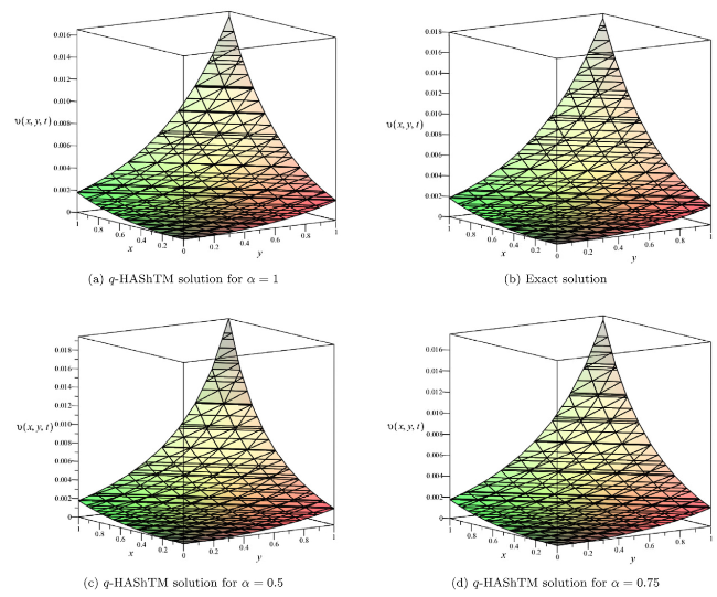
Fig. 1. Surface of Ex. 5.1 at ξ=0.001, ℏ=−1, n=1 and t=0.5. |

Fig. 2. Plot of q-HAShTM solution of Ex. 5.1 at ξ=1., ℏ=−1, n=1, x=0.5 and y=0.5 for different α with respect to t. |
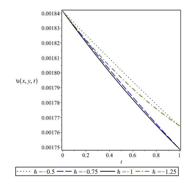
Fig. 3. Plot of q-HAShTM solution of Ex. 5.1 at ξ=0.001, α=1, n=1, x=0.5 and y=0.5 for different ℏ with respect to t. |
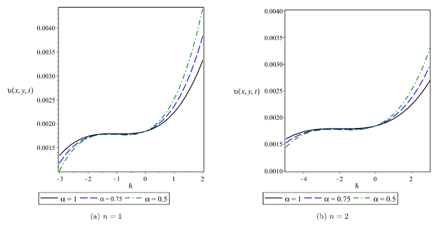
Fig. 4. ℏ-curves for Ex. 5.1 when ξ=0.001., x=0.5, y=0.5 and t=0.5 for two different values of n. |
Table 1. q-HAShTM solution of Ex. 5.1 for distinct value of α at ξ=0.001, ℏ=−1, n=1. |
| x | y | t | α=0.5 | α=0.62 | α=0.75 | α=0.87 | α=1 |
|---|---|---|---|---|---|---|---|
| 0.1 | 0.1 | 0.1 | 5.3174497×10⁻⁵ | 5.3389324×10⁻⁵ | 5.3570296×10⁻⁵ | 5.3697381×10⁻⁵ | 5.3800247×10⁻⁵ |
| 0.25 | 5.2679523×10⁻⁵ | 5.2894786×10⁻⁵ | 5.3104355×10⁻⁵ | 5.3273705×10⁻⁵ | 5.3430769×10⁻⁵ | ||
| 0.5 | 5.2133393×10⁻⁵ | 5.2293910×10⁻⁵ | 5.2475726×10⁻⁵ | 5.2644288×10⁻⁵ | 5.2821787×10⁻⁵ | ||
| 0.75 | 5.1722968×10⁻⁵ | 5.1812209×10⁻⁵ | 5.1934868×10⁻⁵ | 5.2066149×10⁻⁵ | 5.2221467×10⁻⁵ | ||
| 1.0 | 5.1382933×10⁻⁵ | 5.1396611×10⁻⁵ | 5.1446799×10⁻⁵ | 5.1522042×10⁻⁵ | 5.1629975×10⁻⁵ | ||
| 0.5 | 0.5 | 0.1 | 1.8062670×10⁻³ | 1.8141594×10⁻³ | 1.8212709×10⁻³ | 1.8264704×10⁻³ | 1.8307842×10⁻³ |
| 0.25 | 1.7894991×10⁻³ | 1.7958592×10⁻³ | 1.8029738×10⁻³ | 1.8092437×10⁻³ | 1.8153871×10⁻³ | ||
| 0.5 | 1.7744581×10⁻³ | 1.7767885×10⁻³ | 1.7808935×10⁻³ | 1.7856970×10⁻³ | 1.7915096×10⁻³ | ||
| 0.75 | 1.7660272×10⁻³ | 1.7645186×10⁻³ | 1.7647494×10⁻³ | 1.7665935×10⁻³ | 1.7700648×10⁻³ | ||
| 1.0 | 1.7612264×10⁻³ | 1.7564814×10⁻³ | 1.7528562×10⁻³ | 1.7512040×10⁻³ | 1.7512867×10⁻³ | ||
| 1.0 | 1.0 | 0.1 | 1.7797361×10⁻² | 1.6904615×10⁻² | 1.6724702×10⁻² | 1.6809150×10⁻² | 1.6965810×10⁻² |
| 0.25 | 2.2018717×10⁻² | 1.8845028×10⁻² | 1.7233883×10⁻² | 1.6647431×10⁻² | 1.6486041×10⁻² | ||
| 0.5 | 3.2472740×10⁻² | 2.5867778×10⁻² | 2.1231026×10⁻² | 1.8669653×10⁻² | 1.7129980×10⁻² | ||
| 0.75 | 4.5766437×10⁻² | 3.6701664×10⁻² | 2.9054622×10⁻² | 2.3982639×10⁻² | 2.0278570×10⁻² | ||
| 1.0 | 6.1253237×10⁻² | 5.0919452×10⁻² | 4.0794288×10⁻² | 3.3111951×10⁻² | 1.8121814×10⁻² |
Table 2. Comparison between errors of q-HAShTM, VIM [23], FNDM [24] and q-HATM [24] for Ex. 5.1 at ξ=0.001, ℏ=−1, n=1, α=1 and t=1. |
| x | y | q-HAShTM | VIM | FNDM | q-HATM |
|---|---|---|---|---|---|
| 0.02 | 0.02 | 3.00×10⁻⁷ | 7.90×10⁻⁶ | 3.01×10⁻⁷ | 3.01×10⁻⁷ |
| 0.04 | 4.65×10⁻⁷ | 1.19×10⁻⁵ | 4.65×10⁻⁷ | 4.65×10⁻⁷ | |
| 0.06 | 6.34×10⁻⁷ | 1.59×10⁻⁵ | 6.34×10⁻⁷ | 6.34×10⁻⁷ | |
| 0.08 | 8.10×10⁻⁷ | 2.00×10⁻⁵ | 8.10×10⁻⁷ | 8.10×10⁻⁷ | |
| 0.1 | 9.96×10⁻⁷ | 2.41×10⁻⁵ | 9.96×10⁻⁷ | 9.96×10⁻⁷ | |
| 0.06 | 0.02 | 6.34×10⁻⁷ | 1.59×10⁻⁵ | 6.34×10⁻⁷ | 6.34×10⁻⁷ |
| 0.04 | 8.10×10⁻⁷ | 2.00×10⁻⁵ | 8.10×10⁻⁷ | 8.10×10⁻⁷ | |
| 0.06 | 9.96×10⁻⁷ | 2.41×10⁻⁵ | 9.96×10⁻⁷ | 9.96×10⁻⁷ | |
| 0.08 | 1.19×10⁻⁶ | 2.84×10⁻⁵ | 1.19×10⁻⁶ | 1.19×10⁻⁶ | |
| 0.1 | 1.40×10⁻⁶ | 3.27×10⁻⁵ | 1.40×10⁻⁶ | 1.40×10⁻⁶ | |
| 0.1 | 0.02 | 9.96×10⁻⁷ | 2.41×10⁻⁵ | 9.96×10⁻⁷ | 9.96×10⁻⁷ |
| 0.04 | 1.19×10⁻⁶ | 2.84×10⁻⁵ | 1.19×10⁻⁶ | 1.19×10⁻⁶ | |
| 0.06 | 1.40×10⁻⁶ | 3.27×10⁻⁵ | 1.40×10⁻⁶ | 1.40×10⁻⁶ | |
| 0.08 | 1.62×10⁻⁶ | 3.72×10⁻⁵ | 1.63×10⁻⁶ | 1.63×10⁻⁶ | |
| 0.1 | 1.87×10⁻⁶ | 4.18×10⁻⁵ | 1.87×10⁻⁶ | 1.87×10⁻⁶ |
Table 3. Comparison between terms approximation solution of Ex. 5.1 at α=1, ℏ=−1, n=1 and ξ=0.001. |
| x | y | t | 2-term | 3-term | 4-term |
|---|---|---|---|---|---|
| 0.1 | 0.1 | 0.1 | 5.3799579×10⁻⁵ | 5.3800245×10⁻⁵ | 5.3800247×10⁻⁵ |
| 0.5 | 5.2804905×10⁻⁵ | 5.2821566×10⁻⁵ | 5.2821787×10⁻⁵ | ||
| 1.0 | 5.1561562×10⁻⁵ | 5.1628209×10⁻⁵ | 5.1629975×10⁻⁵ | ||
| 0.5 | 0.5 | 0.1 | 1.8306244×10⁻³ | 1.8307817×10⁻³ | 1.8307842×10⁻³ |
| 0.5 | 1.7872672×10⁻³ | 1.7911979×10⁻³ | 1.7915096×10⁻³ | ||
| 1.0 | 1.7330707×10⁻³ | 1.7487934×10⁻³ | 1.7512867×10⁻³ |
The solution of Ex. 5.2 is presented graphically in Fig. 5(a), (b) of Fig. 5 are the graphical simulations of q-HAShTM solution at α=1 and exact solution, respectively and; (c) and (d) are the graphs plotted for solution of Ex. 5.2 for α=0.5 and α=0.75, respectively. Figure 6 and 7 represent the graphical comparison at distinct values of α and distinct values of ℏ, respectively. ℏ-curves for n=1 and n=2 are presented in Fig. 8. Table 4 represents the numerical solutions of Ex. 5.2, at different values of α and variables x, y and t at ξ=0.001, ℏ=−1 and n=1. The comparison between the errors of different methods such as FNDM [25], q-HATM [25] with q-HAShTM is shown in Tables 5. Table 6 represents the terms approximations of the solution of Ex. 5.2.
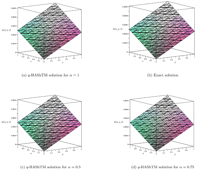
Fig. 5. Surface of Ex. 5.2 at ξ=0.001, ℏ=−1, n=1 and t=0.5. |
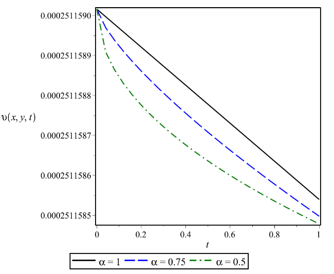
Fig. 6. Plot of q-HAShTM solution of Ex. 5.2 at ξ=0.001, ℏ=−1, n=1, x=0.5 and y=0.5 for different α with respect to t. |
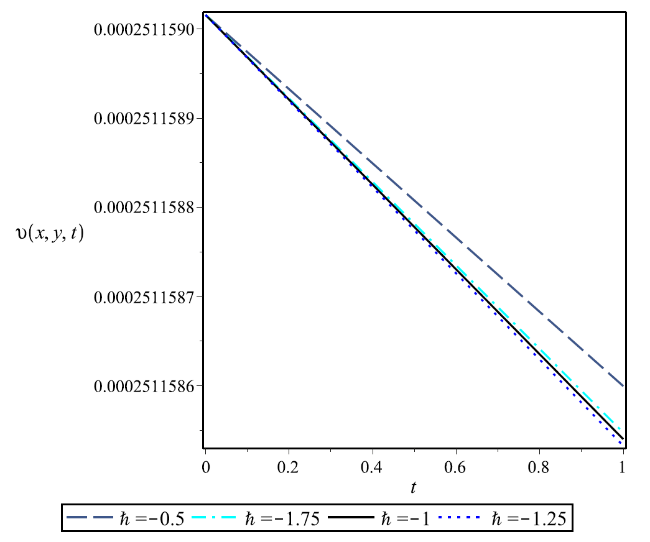
Fig. 7. Plot of q-HAShTM solution of Ex. 5.2 at ξ=0.001, α=1, n=1, x=0.5 and y=0.5 for different ℏ with respect to t. |

Fig. 8. ℏ-curves for Ex. 5.1 when ξ=0.001, x=0.5, y=0.5 and t=0.5 for two different values of n. |
Table 4. q-HAShTM solution of Ex. 5.2 for distinct value of α at ξ=0.001, ℏ=−1, n=1. |
| x | y | t | α=0.5 | α=0.62 | α=0.75 | α=0.87 | α=1 |
|---|---|---|---|---|---|---|---|
| 0.1 | 0.1 | 0.1 | 5.0009124×10⁻⁵ | 5.0009158×10⁻⁵ | 5.0009186×10⁻⁵ | 5.0009206×10⁻⁵ | 5.0009221×10⁻⁵ |
| 0.25 | 5.0009045×10⁻⁵ | 5.0009080×10⁻⁵ | 5.0009114×10⁻⁵ | 5.0009140×10⁻⁵ | 5.0009165×10⁻⁵ | ||
| 0.5 | 5.0008957×10⁻⁵ | 5.0008984×10⁻⁵ | 5.0009014×10⁻⁵ | 5.0009041×10⁻⁵ | 5.0009070×10⁻⁵ | ||
| 0.75 | 5.0008889×10⁻⁵ | 5.0008905×10⁻⁵ | 5.0008927×10⁻⁵ | 5.0008949×10⁻⁵ | 5.0008975×10⁻⁵ | ||
| 1.0 | 5.0008832×10⁻⁵ | 5.0008836×10⁻⁵ | 5.0008847×10⁻⁵ | 5.0008861×10⁻⁵ | 5.0008880×10⁻⁵ | ||
| 0.5 | 0.5 | 0.1 | 2.5115884×10⁻⁴ | 2.5115888×10⁻⁴ | 2.5115892×10⁻⁴ | 2.5115894×10⁻⁴ | 2.5115896×10⁻⁴ |
| 0.25 | 2.5115874×10⁻⁴ | 2.5115879×10⁻⁴ | 2.5115883×10⁻⁴ | 2.5115886×10⁻⁴ | 2.5115889×10⁻⁴ | ||
| 0.5 | 2.5115862×10⁻⁴ | 2.5115867×10⁻⁴ | 2.5115870×10⁻⁴ | 2.5115874×10⁻⁴ | 2.5115877×10⁻⁴ | ||
| 0.75 | 2.5115855×10⁻⁴ | 2.5115857×10⁻⁴ | 2.5115859×10⁻⁴ | 2.5115862×10⁻⁴ | 2.5115865×10⁻⁴ | ||
| 1.0 | 2.5115847×10⁻⁴ | 2.5115848×10⁻⁴ | 2.5115849×10⁻⁴ | 2.5115851×10⁻⁴ | 2.5115853×10⁻⁴ | ||
| 1.0 | 1.0 | 0.1 | 5.0931054×10⁻⁴ | 5.0931061×10⁻⁴ | 5.0931067×10⁻⁴ | 5.0931072×10⁻⁴ | 5.0931075×10⁻⁴ |
| 0.25 | 5.0931038×10⁻⁴ | 5.0931045×10⁻⁴ | 5.0931052×10⁻⁴ | 5.0931058×10⁻⁴ | 5.0931063×10⁻⁴ | ||
| 0.5 | 5.0931019×10⁻⁴ | 5.0931025×10⁻⁴ | 5.0931031×10⁻⁴ | 5.0931037×10⁻⁴ | 5.0931043×10⁻⁴ | ||
| 0.75 | 5.0931004×10⁻⁴ | 5.0931008×10⁻⁴ | 5.0931012×10⁻⁴ | 5.0931017×10⁻⁴ | 5.0931023×10⁻⁴ | ||
| 1.0 | 5.0930992×10⁻⁴ | 5.0930993×10⁻⁴ | 5.0930995×10⁻⁴ | 5.0930998×10⁻⁴ | 5.0931002×10⁻⁴ |
Table 5. Comparison between errors of q-HAShTM, FNDM [25] and q-HATM [25] for Ex. 5.2 at ξ=0.001, n=1, α=1 and ℏ=−1. |
| x | y | t | q-HAShTM | FNDM | q-HATM |
|---|---|---|---|---|---|
| 0.02 | 0.02 | 0.02 | 4.9926×10⁻⁹ | 4.9926×10⁻⁹ | 4.9926×10⁻⁹ |
| 0.04 | 9.9852×10⁻⁹ | 9.9852×10⁻⁹ | 9.9852×10⁻⁹ | ||
| 0.06 | 1.4977×10⁻⁸ | 1.4979×10⁻⁸ | 1.4979×10⁻⁸ | ||
| 0.08 | 1.9970×10⁻⁸ | 1.9970×10⁻⁸ | 1.9970×10⁻⁸ | ||
| 0.1 | 2.4963×10⁻⁸ | 2.4963×10⁻⁸ | 2.4963×10⁻⁸ | ||
| 0.06 | 0.06 | 0.02 | 4.9934×10⁻⁹ | 4.9934×10⁻⁹ | 4.9934×10⁻⁹ |
| 0.04 | 9.9869×10⁻⁹ | 9.9869×10⁻⁹ | 9.9869×10⁻⁹ | ||
| 0.06 | 1.4980×10⁻⁸ | 1.4980×10⁻⁸ | 1.4980×10⁻⁸ | ||
| 0.08 | 1.9973×10⁻⁸ | 1.9974×10⁻⁸ | 1.9974×10⁻⁸ | ||
| 0.1 | 2.4967×10⁻⁸ | 2.4967×10⁻⁸ | 2.4967×10⁻⁸ | ||
| 0.1 | 0.1 | 0.02 | 4.9951×10⁻⁹ | 4.9952×10⁻⁹ | 4.9952×10⁻⁹ |
| 0.04 | 9.9904×10⁻⁹ | 9.9904×10⁻⁹ | 9.9904×10⁻⁹ | ||
| 0.06 | 1.4985×10⁻⁸ | 1.4986×10⁻⁸ | 1.4986×10⁻⁸ | ||
| 0.08 | 1.9980×10⁻⁸ | 1.9981×10⁻⁸ | 1.9981×10⁻⁸ | ||
| 0.1 | 2.4975×10⁻⁸ | 2.4976×10⁻⁸ | 2.4976×10⁻⁸ |
Table 6. Comparison between terms approximation solution of Ex. 5.2 at α=1, ℏ=−1, n=1 and ξ=0.001. |
| x | y | t | 2-term | 3-term | 4-term |
|---|---|---|---|---|---|
| 0.1 | 0.1 | 0.1 | 5.0009221×10⁻⁵ | 5.0009221×10⁻⁵ | 5.0009221×10⁻⁵ |
| 0.5 | 5.0009070×10⁻⁵ | 5.0009070×10⁻⁵ | 5.0009070×10⁻⁵ | ||
| 1.0 | 5.0008880×10⁻⁵ | 5.0008880×10⁻⁵ | 5.0008880×10⁻⁵ | ||
| 0.5 | 0.5 | 0.1 | 2.5115896×10⁻⁴ | 2.5115896×10⁻⁴ | 2.5115896×10⁻⁴ |
| 0.5 | 2.5115877×10⁻⁴ | 2.5115877×10⁻⁴ | 2.5115877×10⁻⁴ | ||
| 1.0 | 2.5115853×10⁻⁴ | 2.5115853×10⁻⁴ | 2.5115853×10⁻⁴ |
7. Conclusion
A robust semi-analytical method, namely q-homotopy analysis Shehu transform approach, is applied to find the solution of Fractional Zakharov-Kuznetsov (2,2,2) and (3,3,3) equations. The graphical and numerical simulations are presented to understand the behaviour of the problem for both of the solutions. As two parameters of q-HAShTM, namely, n and ℏ are very useful for managing the series solution’s convergence. The results show that q-HAShTM is better than the classical methods such as VIM and are similar to other analytical methods such as FNDM and q-HATM. q-HAShTM works on q-HAM technique, which helps to obtain the controlled series solution. The Shehu transform helps solving the fractional-order quickly, allowing the series solution to converge to the exact solution. Finally, it can be concluded that the approach of q-Homotopy analysis Shehu transform method is very effective in understanding the nature of the nonlinear fractional partial differential equation.
Declaration of Competing Interest
The authors declare that they have no known competing financial interests or personal relationships that could have appeared to influence the work reported in this paper.
The authors declare the following financial interests/personal relationships which may be considered as potential competing interests:
Ramakanta Meher
