
1. Introduction and literature review
The ocean and atmosphere are two large reservoirs of water in the earth hydrologic cycle. These two systems are linked to one another by using the coupling conditions. These are responsible for earth’s weather and climate. The ocean helps to regulate temperature in the lower part of the atmosphere. The study of this model is becoming increasingly important in climate change assessment in recent years. Bao et al. [1] was the first find the numerical simulation of air-sea interaction under high wind conditions using coupled model. Then Hallberg [2] found the numerical instability of the ice/ocean coupled system. Beljaars et al. [3] discussed the numerical stability of surface-atmosphere coupling in weather and climate models. An interesting study by Zhang et al. [4], presented the stability analysis of interface conditions for ocean-atmosphere coupling.
In the United State, in community earth system models (CESM) and accelerated climate models for energy (ACME), the earth system elements manage independently. The interaction between their elements is done through an elements called a “coupler” which adapt the information exchange. In ACME the elements are marched forward in time but independently of each other with suitable field using the previous time interval called explicit flux coupling, see Hurrell et al. [5]. The coupling interface model for sea-ice interface see Roberts et al. [6]. For large time steps the coupling model has been discussed in Kushnir et al. [7].
To get the better stability condition Beljaars et al. [3] gives the idea of fully implicit coupling method that uses to estimate the temperature at new time level. The numerical estimation was studied between the surface heat flux and surface temperature. The empirical stability can be obtain via matrix stability analysis which is also given in Zhang et al. [4]. The stability limits in fluid-solid interaction has been studied widely, but small know climate model at large scale that involve complex dynamics. Connors et al. [8] also used various partitioned approaches and focused on the convergence of the numerical scheme. The implicit partitioned technique that does not required the solution of the connected implicit system and have no stability limitations, see Peterson et al. [9].
In an interesting paper on ocean-atmosphere coupling conditions studied by Lemarié et al. [10], they used a nodal based implicit method as well as an explicit cell based method. For the numerical computations and stability analysis a one dimensional diffusion equations with Dirichlet-Neumann (DN)-coupling has been considered in this paper. For the GR-stability they follow the method of Giles [11] to derive the asymptotic stability conditions. They considered air-sea coupling interface interface model and for air-land interface see Beljaars et al. [3].
Zhang et al. [4] studied is also on the ocean-atmosphere coupling. They considered a multi-domain partial differential equation arising in general circulation models used in climate simulations. They claim that in recent years, these two systems became increasingly important in climate change assessment. They also used the explicit and implicit coupling discretization methods in their paper. It was addressed that numerical stability issues arise due to the different time step strategies applied to the coupled partial differential equation. For the stability analysis they also used a GR-stability analysis via the normal mode solutions. Alternatively, to verify their stability results they also calculated the stability via matrix eigenvalue type methods. Further, they point out that the scheme Giles [11] used is not correct.
The authors in [12] discussed (2+1) dimensional Chafee-Infante equation. The analytical solutions and conservation laws using Lie-Backand symmetries. Their study extended the search to breather wave solutions and some other soliton solution. Recently Sun et al. [13] studied the numerical simulation and analysis for the underwater implosion for spherical hollow of ceramic pressure hulls. They considered the compressible multi-phase flow theory and direct numerical simulation. They found that the super imposed effect between spheres exist in the chain reaction implosion which enhanced the implosion shock wave. In another paper Sharma and Mishra [14] studied the well known fluid flow problem modeled using coupled PDEs system. For the numerical simulations they used the Runge-Kutta Felhberg method. Also they studied the effect of various engineering parameters on each other and represented the results via graphical interpretaions.
In this work we study the stability and discrete mass conservation of the two coupling conditions with ocean-atmosphere model given in Zhang et al. [4]. This model the interaction between the ocean and atmospheric regions. This has been coupled by the interface conditions. This modeling gives us a system of partial differential equations with coupling interface conditions. This modeling is used in climate change assessment. A similar study of bi-domain fluid structure has been carried out in Kulkarni et al. [15]. The coupled system with interface conditions is a bit challenging to study numerically. The implicit time integration is becoming more complex as compare to the explicit method. Here, we will use both kind of discretization methods. For studing this problem numerically we can use the large time steps in case of implicit, while smaller time steps for the explicit case. For this, we follow our previous work introduced in Munir [16].
These new solution methods will gives the better idea to understand the stability and mass conservativity for such kind of coupling interface problems. Some of these issues have not been addressed till now in the literature of such kind of coupling conditions. The novel characteristics of the findings from this paper can be of great importance to solve the problem of science and ocean engineering problems numerically.
Organization of the manuscript
The rest of this paper is organized as: The mathematical modeling of the problem with the coupling conditions is given in Section 2. The explicit coupling algorithms for the discretization of the problem will describe in Section 3 and the implicit are given in Section 4. Section 5 applies for discrete mass conservation for the various coupling conditions. Section 6 describes for the stability analysis of the discretized numerical coupling conditions. In Section 7, we summarize the numerical results and discussion and finally the summary and conclusion of this work are given in Section 8.
2. Mathematical modeling
Here we give the mathematical model and numerical dicretization for the ocean-atmosphere model with two coupling interface conditions.
2.1. Ocean-atmosphere model with coupling interface conditions
Now we consider a mathematical model of Zhang et al. [4]. In this study we implement the ocean-atmosphere model with Dirichlet-Neumann coupling, bulk interface coupling condition. We also take a one dimensional diffusion equation for temperature defined on two neighboring domains. The interval $ \Omega=[a, b] $ is considered a domain in one space dimension. We divide the domain into two sub-domains by the mid point $ c=(a+b) / 2 $, which is the common interface boundary. The two sub-domains are $ \Omega_{1}=[a, c] $ and $ \Omega_{2}=[c, b] $. We are interested in interface coupling conditions
$ \frac{\partial v}{\partial t}=k_{-} \frac{\partial^{2} v}{\partial x^{2}} \quad for all \quad v \in \Omega_{1} \times \mathbb{R}_{\geq 0}, \quad \frac{\partial u}{\partial t}=k_{+} \frac{\partial^{2} u}{\partial x^{2}} for all u \in \Omega_{2} \times \mathbb{R}_{\geq 0}. $
for given initial data $ w_{0}: \Omega \rightarrow \mathbb{R} $. We take the outer boundary conditions to be the homogeneous no flux Neumann conditions
$ \frac{\partial}{\partial x} v(a, t)=\frac{\partial}{\partial x} u(b, t)=0 $
and Dirichlet-Neumann coupling interface conditions are given by
$ v(c, t)=u(c, t), \quad \rho_{+} c_{+} k_{+} \frac{\partial u}{\partial z}=\rho_{-} c_{-} k_{-} \frac{\partial v}{\partial z} $
The bulk interface conditions are given
$ k_{-} \frac{\partial v}{\partial x}=b(u-v), \quad k_{+} \frac{\partial u}{\partial x}=b(u-v). $
The eddy diffusivity coefficient defined by $ k_{ \pm}=\frac{\nu_{ \pm}}{\rho_{ \pm} c_{ \pm}} $. The region Ω1 is corresponding to the ocean and Ω2 is to the atmospheric region.
Here ν, ρ and c are the heat diffusion coefficient, density, and heat capacity respectively. The diffusion problem can be rewritten as
$ \rho_{-} c_{-} \frac{\partial v}{\partial t}=\frac{\partial}{\partial x}\left(\nu_{-} \frac{\partial v}{\partial x}\right), \quad \text { for all } \quad v \in \Omega_{1} \times \mathbb{R}_{\geq 0} $
$ \rho_{+} c_{+} \frac{\partial u}{\partial t}=\frac{\partial}{\partial x}\left(\nu_{+} \frac{\partial u}{\partial x}\right), \text { for all } u \in \Omega_{2} \times \mathbb{R}_{\geq 0} $
Neumann condition becomes
$ \nu_{+} \frac{\partial u}{\partial x}=\nu_{-} \frac{\partial v}{\partial x} $
The physical process in the interior of each domain are the independent but there is complex interaction at their common interface. It is necessary to imposed conditions on interface to insure the existence of numerical solution for the coupled system.
3. Coupling algorithms
In this study we will use basically four coupling algorithms: two are explicit and two for the implicit. In the explicit there are two namely explicit nodal based finite difference and explicit cell based finite volume. Also in the implicit there are two one is implicit monolithic and the second one is the partitioned coupling algorithm. First we give the explicit and then the implicit.
3.1. Explicit nodal based coupling algorithm for the DN-coupling
For the numerical discretization we take $ \Omega=[a, b]=[0,1] $. We introduce grid points for the spatio-temporal discretization of the bi-domain ocean-atmosphere on the interval [0,1] with coupling boundary at $ c=\frac{1}{2} $ via a finite difference scheme. We consider N=2m even for some $ m \in \mathbb{N} $ and set $ \Delta x=1 / N $. The Grid points for the two sub-domains $ \Omega_{1}=[0,1 / 2] $ and $ \Omega_{2}=[1 / 2,1] $ are defined as
$ x_{j}=j \Delta x_{-}, \quad for \quad j=0,1, \ldots, m-1 \quad and \quad x_{j}=j \Delta x_{+}, for j=m+1, \ldots, N=2 m. $
At the interface $ c=\frac{1}{2} $ we introduce the double node $ x_{m_{-}}=x_{m_{+}}=m \Delta x $, see Fig. 1. The node $x_{m−}$ is used in conjunction with Ω1 and $x_{m+}$ with Ω2. Later we will make use of cell boundary points $ x_{j \pm \frac{1}{2}}=x_{j} \pm \frac{\Delta x}{2} $. We then consider the nodal values to represent the value of the solution on a cell $ \left[x_{j-\frac{1}{2}}, x_{j+\frac{1}{2}}\right] $.
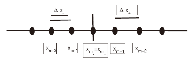
Fig. 1. Grid setting for the Ocean-Atmosphere coupling with nodal based scheme. |
Here we consider an initial and boundary value problem. For this we obtain the scheme at the left hand boundary i.e. j=0 as
$ v_{0}^{n+1}=v_{0}^{n}+2 \gamma_{-}\left(v_{1}^{n}-v_{0}^{n}\right) $
for the interior of the left hand domain i.e. $ 0<j<m $ we obtain
$ v_{j}^{n+1}=v_{j}^{n}+\gamma_{-}\left(v_{j+1}^{n}-2 v_{j}^{n}+v_{j-1}^{n}\right) $
Further the schemes for the Dirichlet-Neumann coupling at j=m i.e. on interface node as
$ \begin{array}{lll} v_{m}^{n+1}=u_{m}^{n}+\gamma_{+}\left(u_{m+1}^{n}-u_{m}^{n}\right)-\gamma_{-}\left(v_{m}^{n}-v_{m-1}^{n}\right) & \text { for } j=m \\ u_{m}^{n+1}=v_{m}^{n+1} & \text { for } j=m \end{array} $
The scheme for the interior of the right sub-domain i.e. $m<j<2m$ is given by
$ u_{j}^{n+1}=u_{j}^{n}+\gamma_{+}\left(u_{j+1}^{n}-2 u_{j}^{n}+u_{j-1}^{n}\right) $
and finally the scheme for the right hand homogeneous Neuman boundary condition as
$ u_{N}^{n+1}=u_{N}^{n}+2 \gamma_{+}\left(u_{N-1}^{n}-u_{N}^{n}\right) \quad j=2 m $
For the purpose of testing the coupling on known solutions we consider the special case $ k_{-}=k_{+}=k $ in (9). Then the coupling should give the single domain solutions. In this case coupling equation will become the standard scheme for the single domain diffusion equation
$ w_{m}^{n+1}=w_{m}^{n}+\gamma\left(\left(w_{m+1}^{n}-w_{m}^{n}\right)-\left(w_{m}^{n}-w_{m-1}^{n}\right)\right) $
Here w will play a role as a single variable in a diffusion PDE in a single domain.
3.1.1. Explicit cell based finite volume discretization for the DN-coupling
The space is discretized on uniform grids with each node denoted by $ x_{j+1 / 2}=(j+1 / 2) \Delta x_{+}, \quad \text { for } j=m, m+1, m+2, \ldots, 2 m $ and $ x_{j+1 / 2}=(j+1 / 2) \Delta x_{-} \quad j=m-1, m-2, \ldots, 1 $. Further the where $ \Delta x_{+} $ and $ \Delta x_{-} $ are the grid spacing. We approximate u and v as follows
$ \begin{aligned} v_{j}^{n} & \approx \frac{1}{\Delta x} \int_{x_{j-\frac{1}{2}}}^{x_{j+\frac{1}{2}}} v\left(x, t_{n}\right) d x, \quad \text { for } \quad j=1, \ldots, m \\ u_{j}^{n} & \approx \frac{1}{\Delta x} \int_{x_{j-\frac{1}{2}}}^{x_{j+\frac{1}{2}}} u\left(x, t_{n}\right) d x, \quad \text { for } \quad j=m+1, \ldots, N=2 m \end{aligned} $
For the discretization of the initial data we can use the integral averages. The integrals may be replaced by a quadrature rule.
Now we write the fully discretized explicit cell base finite volume sys# for the ocean-atmosphere model with Dirichlet-Neumann coupling together as follows. The detail derivation can be found in Munir [16].
$ \begin{array}{ll} v_{1}^{n+1}=v_{1}^{n}+\gamma_{-}\left(v_{2}^{n}-v_{1}^{n}\right) & \text { for } \mathrm{j}=1 \\ v_{j}^{n+1}=v_{j}^{n}+\gamma_{-}\left(v_{j+1}^{n}-v_{j}^{n}\right)-\gamma_{-}\left(v_{j}^{n}-v_{m-1}^{n}\right) & \text { for } 0<\mathrm{j}<\mathrm{m} \\ u_{m}^{n+1}=u_{m}^{n}+\gamma_{+}\left(v_{m+1}^{n}-v_{m}^{n}\right)-\gamma_{-}\left(u_{m}^{n}-u_{m-1}^{n}\right) & \text { for } \mathrm{j}=\mathrm{m} \\ v_{m}^{n+1}=u_{m}^{n+1} & \text { for } \mathrm{j}=\mathrm{m} \\ u_{j}^{n+1}=u_{j}^{n}+\gamma_{+}\left(u_{j+1}^{n}-u_{j}^{n}\right)-\gamma_{+}\left(u_{j}^{n}-u_{m-1}^{n}\right) & \text { for } \mathrm{m}<\mathrm{j}<\mathrm{N} \\ u_{N}^{n+1}=u_{N}^{n}-\gamma_{+}\left(u_{N}^{n}-u_{N-1}^{n}\right) & \text { for } \mathrm{j}=\mathrm{N} \end{array} $
The scheme for the boundary conditions are difference from the explicit nodal based scheme while the schemes for the interior region of the two sub-domain and the coupling conditions are equivalent. Also due to cell discretization we get a one node less than the explicit method. The main difference in the explicit nodal based finite difference and explicit cell based scheme are the discretization on the node in the finite difference and on cells in the finite volume. The difference can be seen in the Figs. 1 and 2.

Fig. 2. Grid setting for the Ocean-Atmosphere coupling with cell based scheme. |
3.2. Bulk interface coupling conditions via explicit cell based finite volume discretization method
Here we give the discretization scheme for the bulk interface conditions. Now for the interface node, i.e. j=m the discretized scheme for the interior of the left sub-domain (8) will take the following flux form
$ v_{m}^{n+1}=v_{m}^{n}+\gamma_{-}\left(v_{m+1}^{n}-v_{m}^{n}\right)-\gamma_{-}\left(v_{m}^{n}-v_{m-1}^{n}\right) $
and the discretized scheme for the right sub-domain (10) will take the form
$ u_{m}^{n+1}=u_{m}^{n}+\gamma_{+}\left(u_{m+1}^{n}-u_{m}^{n}\right)-\gamma_{+}\left(u_{m}^{n}-u_{m-1}^{n}\right). $
We have two ghost point values $ \begin{array}{l} n \\ m-1 \end{array} $ and $ u_{m+1}^{n} $ in the above two formulas. We calculate these values by using the bulk interface coupling conditions given below
$ k_{-} \frac{\partial v}{\partial x}=b(u-v), \quad k_{+} \frac{\partial v}{\partial x}=b(u-v) $
We discretize the first equation of the above equations by using the forward difference approximation and the second equation by the backward difference approximation
$ k_{-} \frac{v_{m+1}^{n}-v_{m}^{n}}{\Delta x}=b\left(u_{m}^{n}-v_{m}^{n}\right), \quad k_{+} \frac{u_{m}^{n}-u_{m-1}^{n}}{\Delta x}=b\left(u_{m}^{n}-v_{m}^{n}\right). $
Solving the first equation for (17) for $ \begin{array}{l} \text { n }\\ m+1 \end{array} $ to obtain $ v_{m+1}^{n}=v_{m}^{n}+\frac{b \Delta x}{k-}\left(u_{m}^{n}-v_{m}^{n}\right) $.
We substitute this value of $ v_{m+1}^{n} $ into (14) to obtain the following formula to determine $ v_{m}^{n+1} $ as follows
$ v_{m}^{n+1}=v_{m}^{n}-\gamma_{-}\left(v_{m}^{n}-v_{m-1}^{n}\right)+\frac{b \Delta t}{\Delta x}\left(u_{m}^{n}-v_{m}^{n}\right) $
Solving the second equation of (17) for $ \begin{array}{l} n \\ m-1 \end{array} $ we get $ v_{m-1}^{n}=v_{m}^{n}-\frac{b \Delta x}{k_{+}}\left(u_{m}^{n}-v_{m}^{n}\right) $. Substituting this into (15) to obtain the following formula to determine $ v_{m}^{n+1} $ as
$ u_{m}^{n+1}=u_{m}^{n}+\gamma_{+}\left(u_{m+1}^{n}-u_{m}^{n}\right)-\frac{b \Delta t}{\Delta x}\left(u_{m}^{n}-v_{m}^{n}\right) $
For $ j \neq m $ we will use the algorithm of DN-coupling discretization. For the bulk interface we will replaced the above two new formulas (18) and (19) in the system (7)–(11). Its means that just the system (9) will change by the above two formulas for j=m.
Bulk interface coupling conditions with explicit central difference approximation
Here we follow exactly the same derivation given above. We approximate the derive of the bulk coupling conditions by central difference method. After simplification we will obtain
$ v_{m}^{n+1}=v_{m}^{n}-2 \gamma_{-}\left(v_{m}^{n}-v_{m-1}^{n}\right)+\frac{2 b \Delta t}{\Delta x}\left(u_{m}^{n}-v_{m}^{n}\right) $
Analogously for the second coupling condition we obtain a scheme for $ w_{m}^{n+1} $
$ u_{m}^{n+1}=u_{m}^{n}+2 \gamma_{+}\left(u_{m+1}^{n}-u_{m}^{n}\right)-\frac{2 b \Delta t}{\Delta x}\left(u_{m}^{n}-v_{m}^{n}\right) $
Again we replacing the Dirichlet-Neumann coupling conditions by the new formulas (20) and (21) for the bulk interface coupling condition.
4. Implicit coupling methods
4.1. Monolithic and partitioned iterative coupling approach
The implicit monolithic approach is similar to the the explicit approach but only difference is to deal the spatial discretization at time level n+1 in implicit. While in the partitioned iterative coupling approach we separate the domain into two sub-sets on which the equations have different constants. Now we make a partition of the two sub-domains. Here we will focus on partitioned iterative coupling approach. For this we follow the steps taken before in our work in Munir [16].
4.1.1. DN-coupling
The discretization for the left sub-domain together with homogeneous Neumann boundary condition and Neumann coupling condition is given by
$ \begin{array}{l} \left(1+2 \gamma_{-}\right) v_{0}^{n+1}-2 \gamma_{-} v_{1}^{n+1}=v_{0}^{n} \quad \text { for } j=0 \\ -\gamma_{-} v_{j-1}^{n+1}+\left(1+2 \gamma_{-}\right) v_{j}^{n+1}-\gamma_{-} v_{j+1}^{n+1}=v_{j}^{n} \quad \text { for } j<m \\ -\gamma_{-} v_{m-1}^{n+1}+\left(1+\gamma_{-}\right) v_{m}^{n+1}=v_{m}^{n}+\gamma_{+}\left(v_{m+1}^{n+1}-v_{m}^{n+1}\right) \quad \text { for } j=m \end{array} $
For the right sub-domain as
$ \begin{array}{rlr} v_{m}^{n+1} & =u_{m}^{n+1} \quad \text { for } j=m \\ -\gamma_{+} u_{j-1}^{n+1}+\left(1+2 \gamma_{+}\right) u_{j}^{n+1}-\gamma_{+} u_{j+1}^{n+1} & =u_{j}^{n} \quad \text { for } j>m \\ -2 \gamma_{+} u_{2 m-1}^{n+1}+\left(1+2 \gamma_{+}\right) u_{2 m}^{n+1} & =u_{2 m}^{n} \quad \text { for } j=2 m \end{array} $
The systems (22) and (23) cannot be solved separately as long as the solution appears on the right hand side. For the convergence of the coupling interface condition we may check the residual equations at the interface $ \begin{array}{l} R_{1}^{n+1}=-\gamma_{-} v_{m-1}^{n+1}+\left(1+\gamma_{-}\right) v_{m}^{n+1}-v_{m}^{n}-\gamma_{+}\left(v_{m+1}^{n+1}-v_{m}^{n+1}\right) \quad \text { and } \\ R_{2}^{n+1}=u_{m+1}^{n+1}-v_{m}^{n+1} \end{array} $ They should become approximately zero. To achieve this we introduce the following sub-iterations. We set $ v_{m}^{n, 0}:=v_{m}^{n}, u_{m}^{n, 0}:=u_{m}^{n} $ and $ u_{m+1}^{n, 0}:=u_{m+1}^{n}. $. Further we introduce the sub-iteration index k=0,1,2,.... With this we modify (22) and (23) to
$ \begin{array}{l} \left(1+2 \gamma_{-}\right) v_{0}^{n, k+1}-2 \gamma_{-} v_{1}^{n, k+1}=v_{0}^{n} \quad \text { for } j=0 \\ -\gamma_{-} v_{j-1}^{n, k+1}+\left(1+2 \gamma_{-}\right) v_{j}^{n, k+1}-\gamma_{-} v_{j+1}^{n, k+1}=v_{j}^{n} \quad \text { for } j<m \\ -\gamma_{-} v_{m-1}^{n, k+1}+\left(1+\gamma_{-}\right) v_{m}^{n, k+1}=v_{m}^{n}+\gamma_{+}\left(u_{m+1}^{n, k}-u_{m}^{n, k}\right) \quad \text { for } j=m \end{array} $
And
$ \begin{array}{llc} u_{m}^{n, k+1} & =u_{m}^{n, k} & \text { for } j=m+1 \\ -\gamma_{+} u_{j-1}^{n, k+1}+\left(1+2 \gamma_{+}\right) u_{j}^{n, k+1}-\gamma_{+} u_{j+1}^{n, k+1} & =u_{j}^{n} \quad \text { for } j>m \\ -2 \gamma_{+} u_{2 m-1}^{n, k+1}+\left(1+2 \gamma_{+}\right) u_{2 m}^{n, k+1} & =u_{2 m}^{n} \quad \text { for } j=2 m. \end{array} $
For the convergence of the coupling interface condition we check the residual equations at the interface
$ \begin{array}{l} R_{1}^{n, k+1}=-\gamma_{-} v_{m-1}^{n, k+1}+\left(1+\gamma_{-}\right) v_{m}^{n, k+1}-\gamma_{+}\left(u_{m+1}^{n, k+1}-u_{m}^{n, k+1}\right)-v_{m}^{n} \text { and } \\ R_{2}^{n, k+1}=v_{m}^{n, k+1}-u_{m}^{n, k+1} \end{array} $
The above iteration process can be repeated. For k→∞ we expect $ R_{1}^{n, k} \rightarrow 0 $ and $ R_{2}^{n, k} \rightarrow 0 $ as well as $ v_{j}^{n, k} \rightarrow v_{j}^{n+1} $ and $ v_{j}^{n, k} \rightarrow v_{j}^{n+1} $, where $ v_{j}^{n+1} $ and $ u_{j}^{n+1} $ are the required solutions.
We prescribe some small tolerance TOL>0 such that when we have achieved $ \left|R_{1}^{n, k+1}\right|<T O L $ and $ \left|R_{2}^{n, k+1}\right|<T O L $ we stop the sub iterations and start the next time step.
Now we want to achieve $ \left|R_{1}^{n, k+1}\right|<T O L $ and $ \left|R_{2}^{n, k+1}\right|<T O L $ for these two system respectively and for large k we expect $ u_{j}^{n, \bar{k}} \rightarrow u_{j}^{n+1} $ and $ v_{j}^{n, k} \rightarrow v_{j}^{n+1} $.
4.1.2. Bulk interface conditions via implicit method
Here we give the schemes for the bulk interface conditions for the implicit coupling discretization method.
One sided finite volume method
The formula for the bulk interface conditions with implicit method is given by
$ -\gamma_{-} u_{m-1}^{n+1}+\left(1+\gamma_{-}+b \frac{\Delta t}{\Delta x}\right) u_{m}^{n+1}-b \frac{\Delta t}{\Delta x} v_{m}^{n+1}=u_{m}^{n} $
and
$ -b \frac{\Delta t}{\Delta x} u_{m}^{n+1}+\left(1+\gamma_{+}+b \frac{\Delta t}{\Delta x}\right) v_{m}^{n+1}-\gamma_{+} v_{m+1}^{n+1}=v_{m}^{n} $
Central difference finite difference method
Analogously we obtain the schemes via the central difference method are
$ -2 \gamma_{-} u_{m-1}^{n+1}+\left(1+2 \gamma_{-}+2 b \frac{\Delta t}{\Delta x}\right) u_{m}^{n+1}-2 b \frac{\Delta t}{\Delta x} v_{m}^{n+1}=u_{m}^{n} $
and
$ -2 b \frac{\Delta t}{\Delta x} u_{m}^{n+1}+\left(1+2 \gamma_{+}+2 b \frac{\Delta t}{\Delta x}\right) v_{m}^{n+1}-2 \gamma_{+} v_{m+1}^{n+1}=v_{m}^{n} $
For the coupled scheme we proceed analogously as the implicit scheme for the Dirichlet-Neumann coupling given in system (22) and (23). We replace the schemes of the Dirichlet-Neumann coupling conditions by the new formulas (27) and (28) for the the one sided and for the central difference (29) and (30). Further for the numerical computations we used the three Algorithms given in our previous work Munir [16].
5. Conservation of the discrete mass for the various coupling conditions
The mass conservation is defined as, under homogeneous Neumann boundary conditions the diffusion equations conserve total mass for concentrations or total energy in the case of the heat equation. Since we assume there are no fluxes across the outer boundaries, the total change of discrete mass or energy in the domain should approximate zero up-to machine accuracy.
This important property must be maintained by the scheme. In order to check whether the mass is conserved throughout the time interval, we compute the total mass $C_{total}$ in the domain at each time step $ t_{n}=n \Delta t $. In this section we derive the discrete mass conservation for the various coupling conditions via explicit discretization methods. First we derive them for the Dirichlet-Neumann coupling and then for the other coupling conditions.
5.1. Dirichlet-Neumann coupling for equal mesh sizes
We follow our previous procedure use for the discrete mass conservation for the DN-coupling given in [16]. In case of the explicit nodal based scheme the total concentration at time $t_{n+1}$ is given by
$ \begin{array}{l} \bar{C}_{\text {total }}^{n+1}= \frac{1}{2} v_{0}^{n+1}+v_{1}^{n+1}+\ldots+v_{m-1}^{n+1}+u_{m}^{n+1}+u_{m+1}^{n+1}+\ldots+\frac{1}{2} u_{N}^{n+1} \\ = \frac{1}{2} v_{0}^{n}+\gamma_{-}\left(v_{1}^{n}-v_{0}^{n}\right)+v_{1}^{n}+\gamma_{-}\left(v_{2}^{n}-v_{1}^{n}\right)-\gamma_{-}\left(v_{1}^{n}-u_{0}^{n}\right) \\ + \ldots+v_{m-1}^{n} \\ +\gamma_{-}\left(v_{m}^{n}-v_{m-1}^{n}\right)-\gamma_{-}\left(v_{m-1}^{n}-v_{m-2}^{n}\right)+u_{m}^{n}+\gamma_{+} \\ \left(u_{m+1}^{n}-u_{m}^{n}\right)-\gamma_{-}\left(u_{m}^{n}-u_{m-1}^{n}\right) \\ +u_{m+1}^{n}+\gamma_{+}\left(u_{m+2}^{n}-u_{m+1}^{n}\right)-\gamma_{+}\left(u_{m+1}^{n}-u_{m}^{n}\right)+\ldots \\ +u_{N-1}^{n}+\gamma_{+}\left(u_{N}^{n}-u_{N-1}^{n}\right)-\gamma_{+}\left(u_{N-1}^{n}-u_{N-2}^{n}\right)+\frac{1}{2} u_{N}^{n} \\ + \gamma_{+}\left(u_{N-1}^{n}-u_{N}^{n}\right) \end{array} $
The identical terms will cancel above and we obtain $ \bar{C}_{\text {total }}^{n+1}=\bar{C}_{\text {total }}^{n} $. This shows that our discretization scheme is conserved.
5.2. DN-coupling for un-equal mesh sizes
In this case we derive the discrete mass conservation for un-equal mesh sizes. This is a bit complex as compare to the equal mesh size. The total concentration in this case will be
$ \begin{array}{l} \bar{C}_{\text {total }}^{0}=c_{-} \Delta x_{-}\left(\frac{1}{2} v_{0}^{0}+v_{1}^{0}+\ldots+v_{m-1}^{0}+\frac{1}{2} v_{m}^{0}\right)+c_{+} \Delta x_{+}\left(\frac{1}{2} u_{m}^{0}\right. \\ \left.+u_{m+1}^{0}+\ldots+u_{N-1}^{0}+\frac{1}{2} u_{N}^{0}\right) \end{array} $
The scheme for the left hand boundary will be
$ \frac{1}{2} v_{0}^{n+1}=\frac{1}{2} v_{0}^{n}+\frac{k_{-} \Delta t}{c_{-}\left(\Delta x_{-}\right)^{2}}\left(v_{1}^{n}-v_{0}^{n}\right) $
and scheme for interior of the left sub-domain is given by
$ v_{j}^{n+1}=v_{j}^{n}+\frac{k_{-} \Delta t}{c_{-}\left(\Delta x_{-}\right)^{2}}\left(v_{j+1}^{n}-v_{j}^{n}\right)-\frac{k_{-} \Delta t}{c_{-}\left(\Delta x_{-}\right)^{2}}\left(v_{j}^{n}-v_{j-1}^{n}\right). $
Now the scheme for DN-coupling
$ u_{m}^{n+1}=u_{m}^{n}+\frac{2 r \gamma_{+}}{1+r}\left(u_{m+1}^{n}-u_{m}^{n}\right)-\frac{2 \gamma_{-}}{1+r}\left(v_{m}^{n}-v_{m-1}^{n}\right). $
Further the scheme for interior of the right sub-domain is
$ u_{j}^{n+1}=u_{j}^{n}+\frac{k_{+} \Delta t}{c_{+}\left(\Delta x_{+}\right)^{2}}\left(u_{j+1}^{n}-u_{j}^{n}\right)-\frac{k_{+} \Delta t}{c_{+}\left(\Delta x_{+}\right)^{2}}\left(u_{j}^{n_{j}}-u_{j-1}^{n}\right) $
and for the right hand boundary condition we have
$ \frac{1}{2} u_{N}^{n+1}=\frac{1}{2} u_{N}^{n}+\frac{k_{+} \Delta t}{c_{+}\left(\Delta x_{+}\right)^{2}}\left(u_{N-1}^{n}-u_{N}^{n}\right) $
Now we write the whole scheme in this form together in a system
$ \begin{array}{l} \frac{c_{-} \Delta x_{-}}{2} v_{0}^{n+1}=\frac{c_{-} \Delta x_{-}}{2} v_{0}^{n}+\frac{k_{-} \Delta t}{c_{-} \Delta x_{-}}\left(v_{1}^{n}-v_{0}^{n}\right) \\ c_{-} \Delta x_{-} v_{j}^{n+1}=c_{-} \Delta x_{-} v_{j}^{n}+\frac{k_{-} \Delta t}{\Delta x_{-}}\left(v_{j+1}^{n}-v_{j}^{n}\right)-\frac{k_{-} \Delta t}{\Delta x_{-}}\left(v_{j}^{n}-v_{j-1}^{n}\right) \\ \frac{c_{-} \Delta x_{-}}{2} v_{m}^{n+1}+\frac{c_{+} \Delta x_{+}}{2} v_{m}^{n+1}=\frac{c_{-} \Delta x_{-}}{2} u_{m}^{n}+\frac{c_{+} \Delta x_{+}}{2} u_{m}^{n} \\ +\frac{k_{+} \Delta t}{\Delta x_{+}}\left(u_{m+1}^{n}-u_{m}^{n}\right) \quad-\frac{k_{-} \Delta t}{\Delta x_{-}}\left(v_{m}^{n}-v_{m-1}^{n}\right) \\ c_{+} \Delta x_{+} u_{j}^{n+1}=c_{+} \Delta x_{+} u_{j}^{n}+\frac{k_{+} \Delta t}{\Delta x_{+}}\left(u_{j+1}^{n}-u_{j}^{n}\right)-\frac{k_{+} \Delta t}{\Delta x_{+}}\left(u_{j}^{n}-u_{j-1}^{n}\right) \\ \frac{c_{+} \Delta x_{+}}{2} u_{N}^{n+1}=\frac{c_{+} \Delta x_{+}}{2} u_{N}^{n}+\frac{k_{+} \Delta t}{\Delta x_{+}}\left(u_{N-1}^{n}-u_{N}^{n}\right) \end{array} $
Clearly after the summation of the above equations the identical terms will cancel out and we obtain a conservative system $ \bar{C}_{\text {total }}^{n+1}=\bar{C}_{\text {total }}^{n} $.
5.3. Bulk interface conditions with one sided nodal explicit discretization method
In this case the total concentration at time $t_{n+1}$ for the ocean-atmosphere model with zero flux boundary conditions on the outer boundaries and with bulk interface coupling conditions is given by
$ \begin{array}{l} \bar{C}_{\text {total }}^{n+1}=\frac{1}{2} u_{0}^{n+1}+u_{1}^{n+1}+\ldots+u_{m-1}^{n+1}+\frac{1}{2} u_{m}^{n+1}+\frac{1}{2} v_{m}^{n+1}+v_{m+1}^{n+1} \\ +\ldots+\frac{1}{2} v_{N}^{n+1} \\ =\frac{1}{2} u_{0}^{n}+\gamma_{-}\left(u_{1}^{n}-u_{0}^{n}\right)+u_{1}^{n}+\gamma_{-}\left(u_{2}^{n}-u_{1}^{n}\right)-\gamma_{-}\left(u_{1}^{n}-u_{0}^{n}\right) \\ +\ldots+v_{m-1}^{n} \\ \quad+\gamma_{-}\left(v_{m}^{n}-v_{m-1}^{n}\right)-\gamma_{-}\left(v_{m-1}^{n}-u_{m-2}^{n}\right) \\ +\frac{1}{2} v_{m}^{n}-\frac{\gamma_{-}}{2}\left(v_{m}^{n}-v_{m-1}^{n}\right)+\frac{\Delta t}{2 \Delta x}\left(u_{m}^{n}-v_{m}^{n}\right) \\ \quad+\frac{1}{2} v_{m}^{n}-\frac{\gamma_{+}}{2}\left(v_{m+1}^{n}-v_{m-1}^{n}\right)-\frac{\Delta t}{2 \Delta x}\left(u_{m}^{n}-v_{m}^{n}\right) \\ +v_{m+1}^{n}+\gamma_{+}\left(v_{m+2}^{n}-v_{m+1}^{n}\right) \\ \quad \quad-\gamma_{+}\left(v_{m+1}-v_{m}^{n}\right)+\ldots+\frac{1}{2} v_{N}^{n}+\gamma_{+}\left(v_{N-1}^{n}-v_{N}^{n}\right). \end{array} $
The identical terms will cancel and we obtain
$ \bar{C}_{\text {total }}^{n+1}=\bar{C}_{\text {total }}^{n}+\frac{\gamma_{-}}{2}\left(u_{m}^{n}-u_{m-1}^{n}\right)-\frac{\gamma_{+}}{2}\left(v_{m+1}^{n}-v_{m}^{n}\right) $
The total concentration $ \bar{C}_{\text {total }}^{n+1} $ does not remain constant. So we concluded that with one sided difference method the discretization is not conserved.
5.4. Bulk interface with central difference method in explicit case
In this case only the schemes for the interface node will be different, i.e. $ v_{m}^{n+1} $ and $ u_{m}^{n+1} $ and the rest of schemes are equal to the Dirichlet-Neumann coupling. The schemes are derived for $ v_{m}^{n+1} $ in (20) and $ u_{m}^{n+1} $ in (21) with central difference approximation. So, the total concentration $C_{\text {total }}^{n+1} \Delta x$ is given by
$\begin{array}{l} \bar{C}_{\text {total }}^{n+1}=\frac{1}{2} v_{0}^{n}+\gamma_{-}\left(v_{1}^{n}-v_{0}^{n}\right)+v_{1}^{n}+\gamma_{-}\left(v_{2}^{n}-v_{1}^{n}\right)-\gamma_{-}\left(v_{1}^{n}-v_{0}^{n}\right) \\ +\ldots+v_{m-1}^{n} \\ +\gamma_{-}\left(v_{m}^{n}-v_{m-1}^{n}\right)-\gamma_{-}\left(v_{m-1}^{n}-u_{m-2}^{n}\right)+\frac{1}{2} u_{m}^{n}-\gamma_{-}\left(u_{m}^{n}-u_{m-1}^{n}\right) \\ +\frac{\Delta t}{\Delta x}\left(u_{m}^{n}-u_{m}^{n}\right) \\ +\frac{1}{2} u_{m}^{n}-\gamma_{+}\left(u_{m+1}^{n}-u_{m}^{n}\right)-\frac{\Delta t}{\Delta x}\left(u_{m}^{n}-u_{m}^{n}\right)+u_{m+1}^{n} \\ +\gamma_{+}\left(u_{m+2}^{n}-u_{m+1}^{n}\right) \\ -\gamma_{+}\left(u_{m+1}^{n}-u_{m}^{n}\right)+\ldots+\frac{1}{2} u_{N}^{n}+\gamma_{+}\left(u_{N-1}^{n}-u_{N}^{n}\right) \end{array}$
The identical terms will cancel in the above expression and we obtain $\bar{C}_{\text {total }}^{n+1}=\bar{C}_{\text {total }}^{n}.$. This shows that the central difference approximation in the case of nodal based explicit maintains the conservativity.
5.5. Bulk interface conditions with one sided difference method (cell based explicit method)
The total concentration at time $t_{n+1}$ for the ocean-atmosphere model with bulk coupling conditions and with zero flux boundary conditions on the outer boundaries the total concentration will be
$\begin{array}{l} \begin{array}{l} \bar{C}_{\text {total }}^{n+1}=\frac{1}{2} v_{0}^{n+1}+v_{1}^{n+1}+\ldots+v_{m-1}^{n+1}+v_{m}^{n+1}+u_{m+1}^{n+1}+\ldots+\frac{1}{2} u_{N}^{n+1} \\ =\frac{1}{2} v_{0}^{n}+\gamma_{-}\left(v_{1}^{n}-v_{0}^{n}\right)+v_{1}^{n}+\gamma_{-}\left(v_{2}^{n}-v_{1}^{n}\right)-\gamma_{-}\left(v_{1}^{n} v_{0}^{n}\right)+\ldots+v_{m-1}^{n} \\ +\gamma_{-}\left(v_{m}^{n}-v_{m-1}^{n}\right)-\gamma_{-}\left(v_{m-1}^{n}-u_{m-2}^{n}\right)+u_{m}^{n}- \\ \gamma_{-}\left(u_{m}^{n}-u_{m-1}^{n}\right)+\frac{\Delta t}{\Delta x}\left(u_{m}^{n}-u_{m}^{n}\right) \\ +u_{m+1}^{n}+\gamma_{+}\left(u_{m+2}^{n}-u_{m+1}^{n}\right)-\gamma_{+}\left(u_{m+1}-u_{m}^{n}\right) \\ +\ldots+\frac{1}{2} u_{N}^{n}+\gamma_{+}\left(u_{N-1}^{n}-u_{N}^{n}\right) \end{array}\\ \bar{C}_{\text {total }}^{n+1}=\frac{1}{2} v_{0}^{n+1}+v_{1}^{n+1}+\ldots+v_{m-1}^{n+1}+v_{m}^{n+1}+u_{m+1}^{n+1}+\ldots+\frac{1}{2} u_{N}^{n+1}\\ =\frac{1}{2} v_{0}^{n}+\gamma_{-}\left(v_{1}^{n}-v_{0}^{n}\right)+v_{1}^{n}+\gamma_{-}\left(v_{2}^{n}-v_{1}^{n}\right)-\gamma_{-}\left(v_{1}^{n} v_{0}^{n}\right)+\ldots+v_{m-1}^{n}\\ +\gamma_{-}\left(v_{m}^{n}-v_{m-1}^{n}\right)-\gamma_{-}\left(v_{m-1}^{n}-u_{m-2}^{n}\right)+u_{m}^{n}-\\ \gamma_{-}\left(u_{m}^{n}-u_{m-1}^{n}\right)+\frac{\Delta t}{\Delta x}\left(u_{m}^{n}-u_{m}^{n}\right)\\ +u_{m+1}^{n}+\gamma_{+}\left(u_{m+2}^{n}-u_{m+1}^{n}\right)-\gamma_{+}\left(u_{m+1}-u_{m}^{n}\right)\\ +\ldots+\frac{1}{2} u_{N}^{n}+\gamma_{+}\left(u_{N-1}^{n}-u_{N}^{n}\right) \end{array}$
Again after cancellation of the like wise terms we get the total concentrations remain constant, i.e. $\bar{C}_{\text {total }}^{n+1}=\bar{C}_{\text {total }}^{n}$. So, we concluded that the central difference with nodal based scheme and one sided with finite volume cell based scheme maintain the conservativity, while the one sided differences with nodal based scheme does not and vice versa.
6. Stability analysis
The stability of numerical schemes is closely associated with the boundedness of numerical solutions, a necessary condition for convergence. To deal the stability analysis for the coupling conditions is a complex process. Here we deal this through Godunov and Ryabenkii stability theory which depends on the normal mode solutions see e.g. [20].
We have to determine whether the coupling conditions give rise to unstable modes even though the CFL condition $0<\gamma_{ \pm} \leq 1$ is satisfied. Further, first we derive the GR-stability for the Dirichlet-Neumann coupling and then for the other coupling conditions with and without ghost point values. The stability for the interior and exterior boundary conditions are given in Munir [16]. For the DN-coupling and bulk interface conditions we gives as follow.
The procedure we use is simpler than the one in Giles [11], Roe et al. [18] and Errera and Chemin [21]. Therefore, we obtain more precise GR-stability results in direct way. The complete coupling system with homogeneous Neumann outer boundary conditions with the ocean-atmosphere model equations can be re-written as follows
$\begin{array}{lc} v_{0}^{n+1}=2 \gamma_{-} v_{1}^{n}+\left(1-2 \gamma_{-}\right) v_{0}^{n} & \text { for } j=0 \\ v_{j}^{n+1}=\gamma_{-} v_{j-1}^{n}+\left(1-2 \gamma_{-}\right) v_{j}^{n}+\gamma_{-} v_{j+1}^{n} & \text { for } 0<j<m \\ \text { the coupling conditions } & \text { for } j=m \\ u_{j}^{n+1}=\gamma_{+} u_{j-1}^{n}+\left(1-2 \gamma_{+}\right) u_{j}^{n}+\gamma_{+} u_{j+1}^{n} & \text { for } m<j<N \\ u_{N}^{n+1}=2 \gamma_{+} u_{N-1}^{n}+\left(1-2 \gamma_{+}\right) u_{N}^{n} & \text { for } j=N. \end{array}$
We consider the following separable normal mode solution for the GR-stability in the case of coupled case
$\begin{aligned} v_{j}^{n}=c_{2} \zeta^{n} q_{2}^{j-m}\left(\gamma_{-}, \zeta\right) & \text { if } j \leq m \\ u_{j}^{n}=c_{1} \zeta^{n} q_{1}^{j-m}\left(\gamma_{+}, \zeta\right) & \text { if } j \geq m \end{aligned}$
For the stability analysis we take the unit open ball $\mathbb{B}=\{z \in \mathbb{C}:|z|<1\}$, where $q_{1}\left(\gamma_{-}, \zeta\right)=q_{2}^{-1}\left(\gamma_{-}, \zeta\right) \in \mathbb{B}, q_{1}\left(\gamma_{+}, \zeta\right)=q_{2}^{-1}\left(\gamma_{+}, \zeta\right) \in \mathbb{B}$.
Here ζ is the temporal amplification factor and $q_{1}\left(\gamma_{+}, \zeta\right)$ as well as $q_{2}\left(\gamma_{-}, \zeta\right)$ are the spatial amplification factors. For the left and right hand boundaries we discussed the GR-stability in the previous subsection. In the right sub-domain, i.e. for j>m the amplitude of the mode $q_{1}^{j-m}\left(\gamma_{+}\right)$ remains bounded as j→∞ due to $\left|q_{1}\left(\gamma_{-}, \zeta\right)\right|<1$. Analogously for the left sub-domain we use $\left|q_{2}\left(\gamma_{-}, \zeta\right)\right|>1$. The discretization is unstable if the difference equation admits such a solutions which gives exponential growth in time, i.e. |ζ|>1.
The stability conditions for the exterior and the interior sub-domain are derived in Munir [16]. Here we only give the derivation of the GR-stability for the Dirichlet-Neumann coupling conditions.
6.1. Dirichlet-Neumann coupling with ghost point value
We discretize the Dirichlet-Neumann coupling with $v_{m}^{n}=u_{m}^{n}$ and one sided differences is given as
$k_{-} \frac{u_{m+1}^{n}-u_{m}^{n}}{\Delta x}=k_{+} \frac{v_{m+1}^{n}-u_{m}^{n}}{\Delta x}=k_{+} \frac{v_{m+1}^{n}-u_{m}^{n}}{\Delta x}$
or
$u_{m+1}^{n}=u_{m}^{n}+\frac{k_{+}}{k_{-}}\left(v_{m+1}^{n}-u_{m}^{n}\right)$
Applying the separable normal mode solutions defined in (35) to the Dirichlet condition $v_{m}^{n}=u_{m}^{n}$ we obtain $v_{m}^{n}=c_{2} \zeta^{n}=u_{m}^{n}=c_{1} \zeta^{n}$. So, the constants c1 and c2 have to be equal, i.e. c1=c2=c.
For simplicity at first we take the identical k−=k+=k. Now we apply the separable normal mode solutions to (36) to obtain the following normal mode equation
$q_{2}(\gamma, \zeta)=1+q_{1}(\gamma, \zeta)-1=q_{1}(\gamma, \zeta)$
This is a contradiction to the far-field assumptions |q2(γ,ζ)|>1 and |q1(γ,ζ)|<1. So, there is no such solution and the coupling condition gives us a stable solution under the Courant–Friedrichs–Lewy (CFL) condition $0<\gamma \leq \frac{1}{2}$.
Alternatively, we proceed as follows by using the discretized scheme of the DN-coupling
$v_{m}^{n+1}=v_{m}^{n}+\gamma_{+}\left(u_{m+1}^{n}-u_{m}^{n}\right)-\gamma_{-}\left(v_{m}^{n}-v_{m-1}^{n}\right).$
Substituting the separable normal mode solution (35) into the above equation leads to the following normal mode equation
$\zeta=1+\gamma_{+}\left(q_{1}\left(\gamma_{+}, \zeta\right)-1\right)-\gamma_{-}\left(1-q_{2}^{-1}\left(\gamma_{-}, \zeta\right)\right)$
We take the modulus of the above equation and use the CFL condition $0 \leq \gamma_{ \pm} \leq \frac{1}{2}$. This implies that 0≤γ−+γ+≤1 which gives us 1−(γ++γ−)≥0. Further we have $q_{2}^{-1}\left(\gamma_{-}, \zeta\right)=q_{1}\left(\gamma_{-}, \zeta\right)$. Then we obtain
$\begin{aligned} |\zeta| & =\left|1-\left(\gamma_{+}+\gamma_{-}\right)+\gamma_{+} q_{1}\left(\gamma_{+}, \zeta\right)+\gamma_{-} q_{1}\left(\gamma_{-}, \zeta\right)\right| \\ & \leq\left|1-\left(\gamma_{+}+\gamma_{-}\right)\right|+\gamma_{+}\left|q_{1}\left(\gamma_{+}, \zeta\right)\right|+\gamma_{-}\left|q_{1}\left(\gamma_{-}, \zeta\right)\right| \\ & \leq 1-\left(\gamma_{+}+\gamma_{-}\right)+\gamma_{+}+\gamma_{-} \\ & \leq 1 \end{aligned}$
Therefore, this coupling condition does not introduce instabilities when the CFL condition is satisfied.
Note that in all cases we could alternatively do the stability analysis for the discrete coupling condition itself as well as for its use in a modification of the scheme. Here we are not able to prove the stability for the coupling itself using only the properties |q1|<1 and |q2|>1.
6.2. GR-stability for the bulk coupling
Bulk coupling conditions via one sided differences for the finite volume scheme
First we derive the GR-stability for the one sided finite volume schemes. The discretized coupling scheme for the bulk coupling conditions was derived in (18)
$v_{m}^{n+1}=v_{m}^{n}-\gamma_{-}\left(v_{m}^{n}-v_{m-1}^{n}\right)+\frac{b \Delta t}{\Delta x}\left(u_{m}^{n}-v_{m}^{n}\right)$
We take the modulus of the above normal mode equation under the CFL condition. Using $q_{2}^{-1}\left(\gamma_{-}, \zeta\right)=q_{1}\left(\gamma_{-}, \zeta\right)$ we obtain
$\begin{aligned} |\zeta| & \leq\left|1-\gamma_{-}\right|+\gamma_{-}\left|q_{1}\left(\gamma_{-}, \zeta\right)+\frac{b \Delta x}{D_{-}} \frac{\left(c_{1}-c_{2}\right)}{c_{2}}\right| \\ & \leq 1-\gamma_{-}+\gamma_{-}\left|q_{1}\left(\gamma_{-}, \zeta\right)+\frac{b \Delta x}{D_{-}} \frac{\left(c_{1}-c_{2}\right)}{c_{2}}\right| \end{aligned}$
Now $\left|q_{1}\left(\gamma_{-}, \zeta\right)+\frac{b \Delta x}{D_{-}} \frac{\left(c_{1}-c_{2}\right)}{c_{2}}\right| \leq\left|q_{1}\left(\gamma_{-}, \zeta\right)\right|+\left|\frac{b\left(c_{1}-c_{2}\right)}{c_{2}}\right| \frac{\Delta x}{D_{-}} \leq 1$ for Δx small enough. So we get the required condition |ζ|≤1 for the GR-stability under the CFL condition. Analogously we can derive the same stability condition for the second scheme of the coupling condition corresponding to the right hand domain.
Bulk coupling conditions via central differences
Now we use the bulk coupling condition for $u_{m}^{n+1}$ that was derived in (20)
$v_{m}^{n+1}=v_{m}^{n}-2 \gamma_{-}\left(v_{m}^{n}-v_{m-1}^{n}\right)+\frac{2 b \Delta t}{\Delta x}\left(u_{m}^{n}-v_{m}^{n}\right)$
After applying the normal mode solutions to the above scheme we obtain the following normal mode equation
$\begin{aligned} |\zeta| & \leq\left|1-2 \gamma_{-}\right|+2 \gamma_{-}\left|q_{1}\left(\gamma_{-}, \zeta\right)+\frac{b \Delta x}{D_{-}} \frac{\left(c_{1}-c_{2}\right)}{c_{2}}\right| \\ & \leq 1-2 \gamma_{-}+2 \gamma_{-}\left|q_{1}\left(\gamma_{-}, \zeta\right)+\frac{b \Delta x}{D_{-}} \frac{\left(c_{1}-c_{2}\right)}{c_{2}}\right| \end{aligned}$
To follow the same argument which is used just above here too. Then we obtain the GR-stability condition |ζ|≤1. Analogously, we can derive the GR-stability for the second scheme of the bulk coupling conditions.
7. Numerical results and discussion
Here we give the numerical results of the discrete mass conservation and stability of the coupling conditions considered in this study. We use the values for the numerical computations given in Table 1.
Table 1. The basic parameters used in the numerical computations of the ocean-atmosphere coupling model. The values have been taken from Zhang et al. [4]. |
| Regions | Parameters | Description | Value | Unit |
|---|---|---|---|---|
| ρ+ | density | 1 | kgm−3 | |
| c+ | heat capacity | 1000 | J kg−1 K−1 | |
| Atmosphere | ν+ | dynamic diffusitvity | 300 | J s−1 m−1 K−1 |
| k+ | eddy diffusitivity | 300000 | m2 s−1 | |
| N+ | grid points | 200 | ||
| γ+ | parabolic CFL | 3.333e-01 | ||
| ρ− | density | 1000 | kgm−3 | |
| c− | heat capacity | 400 | J kg−1 K−1 | |
| Ocean | ν− | diffusion coefficient | 4×10⁵ | m2 s−1 |
| k− | eddy diffusitivity | 160000 | ||
| N− | grid points | 200 | ||
| γ− | parabolic CFL | 1.777e-01 | ||
| b | bulk coefficient | [5, 100] | J s−1 m2 K−1 |
7.1. DN-coupling with un-equal diffusion coefficients
Now we give the numerical results for the DN-coupling via explicit, implicit methods with ocean-atmosphere model equations for the parameters given in Table 1.
7.1.1. Test case 1, for the cosine initial data
Here we compute the solution of DN-coupling for un-equal diffusion coefficients via explicit and implicit discretization methods. The implicit coupling methods have further two methods namely: implicit monolithic and implicit partitioned coupling iterative approach. These results are plotted in Fig. 3 with initial data $u_{0}(x)=\cos (\pi x)+1$ and mesh size Δx=1/200.
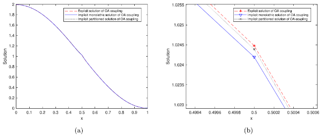
Fig. 3. Comparison of the ocean-atmosphere with DN-coupling conditions via the explicit, implicit monolithic, implicit partitioned iterative coupling approaches and with un-equal diffusion coefficients k−≠k+ for the sine initial data. |
Again the results are not clearly distinguishable. So, we zoom in at the interface of the figure given in the left panel. It is given in the right panel of the Fig. 3. The three solutions of our DN-coupling schemes are near to each. This gives us a good agreement between the three solutions. This can be seen in the left panel of Fig. 3. This difference of the solutions will be explained for the discrete mass conservation in the Section 7.2.
7.1.2. Test case 2, for the piecewise constant initial data
Also we plot the solution of the DN-coupling via explicit, implicit coupling methods for the piecewise constant initial data v0(x)=0.04 for x∈[0,1/2] and v0(x)=600 for x∈[1/2,1]. The remaining data for these computations are the same as used above. We found a good agreement between our numerical solutions. The results are given in Fig. 4. The results are not distinguishable so we zoom in at the interface of the solutions which is given in Fig. 5.
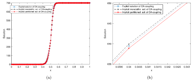
Fig. 4. Comparison of ocean-atmosphere: with DN-coupling conditions via the explicit, implicit monolithic, implicit partitioned iterative coupling approaches with un-equal k−≠k+ for the piecewise constant initial data, while the figure in the right panel is zoom into the numerical solutions near x=0.5 in the upper part. |
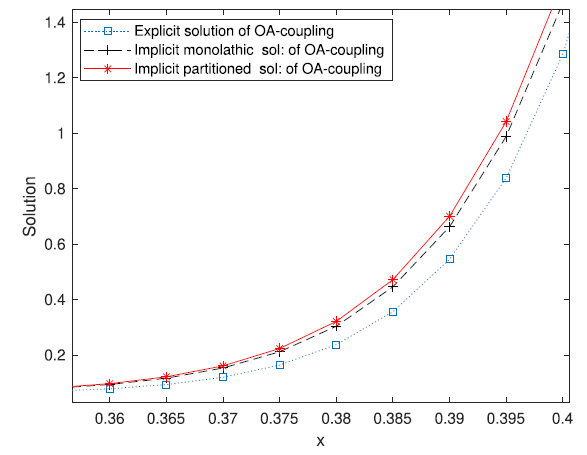
Fig. 5. Further zoom: into the lower numerical solutions in Fig. 4 (b) at x=0.5 in the lower part. |
7.1.3. The stable and unstable solutions for the bulk coupling conditions
We use the initial data $u_{0}(x)=\cos (\pi x / L)+1$ for x∈[0,1/2] and $v_{0}(x)=\cos (\pi x / L)+1$1 for x∈[1/2,1], the diffusion coefficients, γ−=0.001 and γ+=0.003. Here, we calculate the results for the bulk coupling with explicit nodal based discretization method. Note that for the mesh size Δx=1/200 we obtain an unstable solution. This is shown in the left panel of the Fig. 6. While we obtain the stable solutions for Δx=1/400 and higher which is shown in the right panel of Fig. 6.
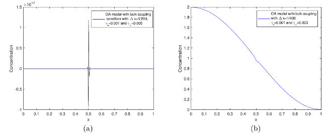
Fig. 6. Unstable and stable solutions: for the ocean-atmosphere model with bulk interface conditions via explicit nodal based method. |
7.2. Discrete mass conservation for the ocean-atmosphere model equations with various coupling conditions
The numerical results for the bi-domain diffusion equations with various coupling conditions will give in this section.
7.2.1. DN-coupling scheme
Here we present the result for the numerical values given in the Table 1. We will compare our results of the DN-coupling of explicit and implicit. These are given as follows. First we give the results of our DN-coupling scheme for the initial data $v_{0}(x)=\sin (\pi x)+1$1 and then for a piecewise continuous initial data v0(x)=0.04, v0(x)=600 and spatial step size Δx=1/2000. The results are given in table form in Fig. 2. The plot for the sine initial data can be seen in Fig. 7 and for the piecewise constant data in Fig. 8.
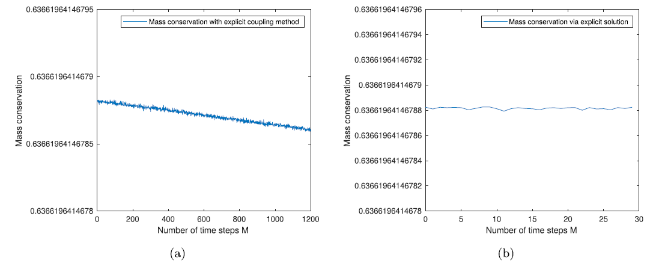
Fig. 7. Ocean-atmosphere with DN-coupling k−≠k+: The figure in the left panel is the result for the DN-coupling of our scheme with initial data v0(x)=sin(πx)+1 for the first 30 time steps and the figure in the right panel is for M=1200 number of time steps, Δx=1/2000 and with un-equal k±. |
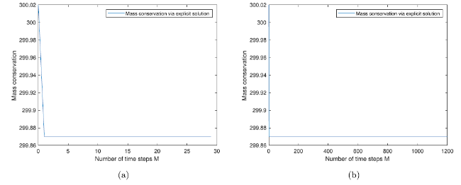
Fig. 8. Ocean-atmosphere with DN-coupling for piecewise constant initial data: The figure in the left panel is the result of the DN-coupling with initial data v0(x)=0.04 for x∈[0,1/2] and v0(x)=600 for x∈[1/2,1] for the first 30 number time steps and the figure in the right panel is for the M=1200 number of time steps, Δx=1/2000 and with un-equal k±. |
Table 2. Ocean-Atmosphere with DN-coupling k−≠k+: Table for the total concentration for the DN-coupling scheme via explicit coupling method with initial data v0(x)=sin(πx) and with a constant data v0(x)=0.04, v0(x)=600 and for the rest of the numerical values given in Table 1. |
| Number of time steps n | OA-coupling(sine data) | OA-coupling(constant data) |
|---|---|---|
| 0 | 6.366196414678824e-01 | 3.000200000000000e+02 |
| 200 | 6.366196414678791e-01 | 2.998700099999999e+02 |
| 400 | 6.366196414678791e-01 | 2.998700099999996e+02 |
| 600 | 6.366196414678714e-01 | 2.998700099999992e+02 |
| 800 | 6.366196414678681e-01 | 2.998700099999988e+02 |
| 1000 | 6.366196414678654e-01 | 2.998700099999984e+02 |
| 1200 | 6.366196414678603e-01 | 2.998700099999979e+02 |
7.2.2. Results of the discrete mass conservation for the bulk interface conditions
As we explained in the derivation of the discrete mass conservation that the discretizations of the boundary conditions as well as the interface conditions via one sided methods does not maintain the conservativity, while the central difference method maintains the conservativity. Now here we show this through numerical values and plots.
First we calculate the total mass for the bulk interface conditions via one sided and central difference method for the initial data v0(x)=cos(πx)+1. We took un-equal diffusion coefficients k− and k+, with Δx=1/2000. The values for different time steps are given in table in Fig. 3. The plots for the one sided method can be seen in Fig. 9 and the plots for the central difference is given in Fig. 10.
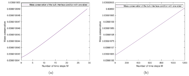
Fig. 9. Ocean-atmosphere with bulk interface conditions: The figure in the left panel is for the bulk interface conditions via one sided difference with $u_{(0)}=\sin (\pi x)$ for the first 30 time steps and the figure in the right panel is for the number of time steps M=1200 and Δx=1/2000. |
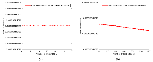
Fig. 10. Ocean-atmosphere with bulk interface coupling conditions: The figure in the left panel is for the bulk interface conditions via central difference with piecewise constant $v_{0}(x)=\sin (\pi x)$ for the first 30 time steps and the figure in the right panel is for the number of time steps M=1200 and Δx=1/2000. |
Table 3. Ocean-atmosphere with bulk interface conditions: Table for the total concentration for the bulk interface conditions via one sided and central difference methods with explicit coupling method with initial data $v_{0}(x)=\sin (\pi x)+1$, with distinct diffusion coefficients and with Δx=1/2000. |
| No.of TS n | OA-coupling (sine data with one sided) | OA-coupling(sine data with central) |
|---|---|---|
| 0 | 6.366196414678824e-01 | 6.366196414678824e-01 |
| 200 | 6.366196999020228e-01 | 6.366196414678793e-01 |
| 400 | 6.366197609117078e-01 | 6.366196414678744e-01 |
| 600 | 6.366198223852731e-01 | 6.366196414678709e-01 |
| 800 | 6.366198840951384e-01 | 6.366196414678682e-01 |
| 1000 | 6.366199459530066e-01 | 6.366196414678661e-01 |
| 1200 | 6.366200079135517e-01 | 6.366196414678605e-01 |
Also we used the piecewise continuous initial data v0(x)=0.04 and v0(x)=600 for both methods. The numerical values for the different time steps are presented in Fig. 4. The plots for the one sided difference are given in Fig. 11 and for central difference method in Fig. 12. From these tables and graphical representations again we conclude that the one sided difference nodal based clearly does not maintain the conservativity for the finite difference case, while the one sided finite volume cell based scheme maintains. Further the central difference maintains discrete mass conservativity.
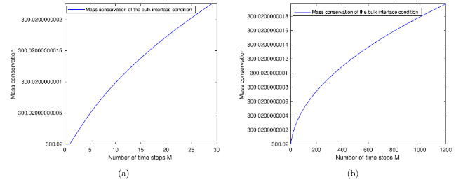
Fig. 11. Ocean-atmosphere with bulk interface coupling conditions: The figure in the left panel is for the bulk interface conditions via one sided difference with piecewise constant initial data v0(x)=0.04 and v0(x)=600 for first 30 time steps and the figure in the right panel is for the number of time steps M=1200 and Δx=1/2000. |
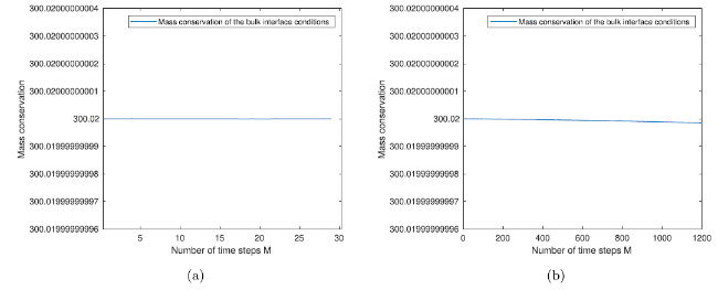
Fig. 12. Ocean-atmosphere with bulk interface coupling conditions: The figure in the left panel is for the bulk interface conditions via central difference for the initial data v0(x)=0.04 and v0(x)=600 for first 30 time steps and the figure in the right panel is for M=1200 number of time steps and Δx=1/2000. |
Table 4. Ocean-atmosphere with bulk interface conditions: Table for the total concentration for the bulk interface conditions via one sided and central difference methods with explicit coupling method with piecewise constant data (PCD) v0 (x)=0.04, v0 (x)=600 with distinct diffusion coefficients and with Δx=1/2000. |
| No.of TS n | OA-coupling with one sided PCD | OA-coupling with central PCD |
|---|---|---|
| 0 | 3.000200000000000e+02 | 3.000200000000000e+02 |
| 200 | 3.000200000007450e+02 | 3.000199999999999e+02 |
| 400 | 3.000200000010960e+02 | 3.000199999999997e+02 |
| 600 | 3.000200000013655e+02 | 3.000199999999995e+02 |
| 800 | 3.000200000015929e+02 | 3.000199999999992e+02 |
| 1000 | 3.000200000017932e+022 | 3.000199999999988e+02 |
| 1200 | 3.000200000019742e+02 | 3.000199999999986e+02 |
8. Summary and conclusion
In this paper we studied the discrete mass conservation and stability characteristics of the ocean-atmosphere model with two coupling conditions. For the numerical study, we used two kinds of coupling strategies namely, explicit coupling and implicit coupling discretization methods. These methods include the explicit nodal based coupling, explicit cell based, implicit monolithic and implicit partitioned coupling approaches. We concluded that some of the discretization methods maintain the discrete mass conservation and others are not. In this, the explicit finite volume maintain the discrete mass conservation via one sided approximation method, while the explicit finite difference maintain the conservation with the central difference approximation.
The stability analysis has been discussed with the well known GR-Stability method which is based on the normal mode analysis. We obtained an exact condition for stability. In previous literature the asymptotic stability that is based on various assumptions are used to obtain the stability conditions. The impact of stability seems to depend on the diffusion coefficients, CFL numbers heat capacities, eddy diffusitivity and especially the numerical discretization scheme. As we know, the explicit method is conditionally stable, while the implicit is unconditionally stable. We showed in this work, that the Dirichlet-Neumann condition imposed on the two coupled component does not affect the stability for the explicit coupling as well as for the implicit. While in the case of bulk interface conditions we obtain an unstable solution for the larger step size and a stable solution for smaller step size.
For the verification of the numerical results and testing our algorithm for the well-known initial data, we performed our numerical solutions. So, it is concluded that our numerical schemes obey the well-known initial data, which implies that our schemes are correct. It is important to state that the choice of values for k−, k+, ρ± and ν± are arbitrary. It depends on the problem and material property. The results of the analysis for the one dimensional diffusion model is also applicable to real three dimensional models, because the heat and turbulence in the ocean-atmosphere circulation transfer mainly in the vertical direction. This vertical one dimensional case can be considered as one slice from the three dimensional model along the vertical direction. The whole domain can be covered with parallel computations.
This research has applied numerical techniques for solving complex coupled partial differential equations (PDEs) with interface conditions. Most ocean engineering problems which are modeled using coupled PDEs can also apply our techniques. This will provide better interpretation for modeling physical ocean engineering models. Most of our numerical results are based on the sine or cosine functions, which gives us waves pattern in the respective sub-region.
Declaration of Competing Interest
The authors declare that there are no conflicts of interest regarding the publication of this paper.
Acknowledgment
The authors extend their appreciation to the Deans of Scientific Research at King Khalid University, Abha, Saudi Arabia for funding this work through research group program under grant number GRP-216/1443.
