
1. Introduction
Coupled system is usually composed of two or more ordinary differential equations, partial differential equations or fractional partial differential equations. The coupled system usually comes from the fields of fluid dynamics, ocean physics, marine engineering, control theory, control engineering and communication system. This kind of system is a very important mathematical and physical equations. This year’s research shows that many experts and scholars are devoted themselves to the research of coupled system. For example, the well-known coupled Schröding equations [1], [2], coupled Boussinesq equations [3], coupled KdV equations [4], coupled nonlinear Maccari system [5] and coupled Fokas-Lenells system [6]. Among them, the most striking is to construct the traveling wave solution [7], [8], [9], [10], [11], [12], [13], [14], [15], [16], [17] of the coupled system.
$\left\{\begin{array}{l} i D_{\tau} \frac{\partial u}{\partial x}+\frac{\sigma}{2} \frac{\partial^{2} u}{\partial \tau^{2}}+\gamma_{1}\left(2|u|^{2}+|v|^{2}\right) D_{\tau} u+\gamma_{1} u v^{*} D_{\tau} v=0 \\ i D_{\tau} \frac{\partial v}{\partial x}+\frac{\sigma}{2} \frac{\partial^{2} v}{\partial \tau^{2}}+\gamma_{2}\left(2|v|^{2}+|u|^{2}\right) D_{\tau} u+\gamma_{2} v u^{*} D_{\tau} u=0 \end{array}\right.$
where $u=u(τ,x) $ and $v=v(τ,x) $ stand for the complex envelopes of the double field components. $τ$ and $x$ represent the time and continuous distance, respectively. The differential operator $D_τ$ is defined by $D_{\tau}=1+i \varepsilon(\partial / \partial \tau)$ (here ε⩾0). σ represents the group velocity dissipation parameter. $γ_1$ and $γ_2$ represent nonlinear coefficients.
The FL system is an integrable generalization of the nonlinear Schrödinger equation [20], [21], [22], [23], [24], [25], which is one of the topics of recent research. It is worth noting that the FL system is obtained by Fokas [26] from a mathematical point of view by employing two Hamiltonian operators related to the nonlinear Schrödinger equation and by Lenells [27] from the perspective of physics starting from the Maxwell’s equations. The FL system is usually used to simulate the propagation of ultrashort optical pulses in birefringent fibers or crossing sea waves on the high seas. Therefore, it is particularly important to study the optical soliton [28], [29], [30], [31], [32] and traveling wave solution [33], [34], [35], [36] of the FL system. Recently, some interesting results have been reported. For example, in Triki et al. [19], Triki et al.obtained the chirped optical soliton of the FL system in birefringent fiber meduium. In [37], chen et al.regarded the study of peregrine solitons of the FL system as a very important topic. In [38], by using the extended trial function method, the optical soliton solutions of the FL system in birefringent fibers were obtained.
In present section, we mainly introduce the research background and research progress of the coupled Fokas-Lenells system. In the following work, we construct the single traveling wave solutions for the coupled Fokas-Lenells system by using the polynomial complete discriminant system method. In Section 3, we give a summary.
2. Single traveling wave solutions for (1.1)
In order to construct the optical solitons and single traveling wave solutions of (1.1), we firstly take into account the following traveling wave transformation
$\begin{aligned} u(\tau, x) & =P(\zeta) e^{i\left(\psi_{1}(\zeta)-k_{1} x\right)}, v(\tau, x)=Q(\zeta) e^{i\left(\psi_{2}(\zeta)-k_{2} x\right)} \\ \zeta & =\tau-\alpha x \end{aligned}$
where the parameters $P(ζ) $ and $Q(ζ) $ represent the amplitudes. $ψ_1$ and $ψ_2$ are real functions with respect to variable ζ.
Plugging (2.1) into (1.1) and separating the real and imaginary part, we obtain
$\begin{aligned} \frac{\sigma+2 \alpha \varepsilon}{2} \frac{d^{2} P}{d \zeta^{2}} & -\frac{\sigma+2 \alpha \varepsilon}{2} P\left(\frac{d \psi_{1}}{d \zeta}\right)^{2}+\left(\alpha-\varepsilon k_{1}\right) P \frac{d \psi_{1}}{d \zeta} \\ & +2 \gamma_{1} P\left(P^{2}+Q^{2}\right)+k_{1} P-\varepsilon \gamma_{1}\left(2 P^{2}+Q^{2}\right) P \frac{d \psi_{1}}{d \zeta} \\ & -\varepsilon \gamma_{1} P Q^{2} \frac{d \psi_{2}}{d \zeta}=0 \end{aligned}$
$\begin{array}{l} \frac{\sigma+2 \alpha \varepsilon}{2}\left(P \frac{d^{2} \psi_{1}}{d \zeta^{2}}+2 \frac{d P}{d \zeta} \frac{d \psi_{1}}{d \zeta}\right)-\left(\alpha-\varepsilon k_{1}\right) \frac{d P}{d \zeta} \\ \quad+2 \varepsilon \gamma_{1} P^{2} \frac{d P}{d \zeta}+\varepsilon \gamma_{1}\left(Q^{2} \frac{d P}{d \zeta}+P Q \frac{d Q}{d \zeta}\right)=0 \end{array}$
$\begin{aligned} \frac{\sigma+2 \alpha \varepsilon}{2} \frac{d^{2} Q}{d \zeta^{2}} & -\frac{\sigma+2 \alpha \varepsilon}{2} P\left(\frac{d \psi_{2}}{d \zeta}\right)^{2}+\left(\alpha-\varepsilon k_{2}\right) Q \frac{d \psi_{2}}{d \zeta} \\ & +2 \gamma_{2} Q\left(P^{2}+Q^{2}\right)+k_{2} Q-\varepsilon \gamma_{2}\left(2 Q^{2}+P^{2}\right) Q \frac{d \psi_{2}}{d \zeta} \\ & -\varepsilon \gamma_{2} Q P^{2} \frac{d \psi_{1}}{d \zeta}=0 \end{aligned}$
$\begin{array}{l} \frac{\sigma+2 \alpha \varepsilon}{2}\left(Q \frac{d^{2} \psi_{1}}{d \zeta^{2}}+2 \frac{d Q}{d \zeta} \frac{d \psi_{2}}{d \zeta}\right)-\left(\alpha-\varepsilon k_{2}\right) \frac{d Q}{d \zeta} \\ \quad+2 \varepsilon \gamma_{2} Q^{2} \frac{d Q}{d \zeta}+\varepsilon \gamma_{2}\left(P^{2} \frac{d Q}{d \zeta}+Q P \frac{d P}{d \zeta}\right)=0 \end{array}$
Multiplying both sides of Eq. (2.3) by $P$ and integrating it once, we have
$\frac{d \psi_{1}}{d \zeta}=\frac{\alpha-\varepsilon k_{1}}{\sigma+2 \alpha \varepsilon}-\frac{\varepsilon \gamma_{1}}{\sigma+2 \alpha \varepsilon}\left(P^{2}+Q^{2}\right)$
Similar to (2.6), multiplying both sides of Eq. (2.5) by $Q$ and integrating it once, we obtain
$\frac{d \psi_{2}}{d \zeta}=\frac{\alpha-\varepsilon k_{2}}{\sigma+2 \alpha \varepsilon}-\frac{\varepsilon \gamma_{2}}{\sigma+2 \alpha \varepsilon}\left(P^{2}+Q^{2}\right)$
Integrating both sides of Eqs. (2.6) and (2.7) simultaneously and making the integration constant zero, hence, we can give the corresponding phase shifts of the two involved waves
$\psi_{1}(\zeta)=\delta_{1} \zeta-\eta_{1} \int\left(P^{2}+Q^{2}\right) d \zeta$
$\psi_{2}(\zeta)=\delta_{2} \zeta-\eta_{2} \int\left(P^{2}+Q^{2}\right) d \zeta$
where $\delta_{1}=\frac{\alpha-\varepsilon k_{1}}{\sigma+2 \alpha \varepsilon}, \delta_{2}=\frac{\alpha-\varepsilon k_{2}}{\sigma+2 \alpha \varepsilon}, \eta_{1}=\frac{\varepsilon \gamma_{1}}{\sigma+2 \alpha \varepsilon}$ and $\eta_{2}=\frac{\varepsilon \gamma_{2}}{\sigma+2 \alpha \varepsilon}$.
Substituting (2.8) and (2.9) into (2.2) and (2.4) respectively, we can get
$\left\{\begin{array}{l} \frac{d^{2} P}{d \zeta^{2}}+a_{1} P^{5}+a_{2} P^{3}+a_{3} P Q^{2}+a_{4} P^{3} Q^{2}+a_{5} P Q^{4}+a_{6} P=0 \\ \frac{d^{2} Q}{d \zeta^{2}}+b_{1} Q^{5}+b_{2} Q^{3}+b_{3} Q P^{2}+b_{4} Q^{3} P^{2}+b_{5} Q P^{4}+b_{6} Q=0 \end{array}\right.$
where the parameters $a_i$ and $b_i (i=1,…,6)$ are given by $a_{1}=3 \eta_{1}^{2}$, $a_{2}=\kappa_{3}-4 \eta_{1} \delta_{1}, a_{3}=\kappa_{3}-2 \eta_{1} \delta_{1}-2 \eta_{1} \delta_{2}, a_{4}=2 \eta_{1} \eta_{2}+4 \eta_{1}^{2}, a_{5}=2 \eta_{1} \eta_{2}+\eta_{1}^{2}$, $a_{6}=\kappa_{1}+\delta_{1}^{2}, b_{1}=3 \eta_{2}^{2}, b_{2}=\kappa_{4}-4 \eta_{4} \delta_{4}, b_{3}=\kappa_{4}-2 \eta_{2} \delta_{2}-2 \eta_{2} \delta_{1}$, $b_{4}=2 \eta_{1} \eta_{2}+4 \eta_{2}^{2}, b_{5}=2 \eta_{1} \eta_{2}+\eta_{2}^{2}$ and $b_{6}=\kappa_{2}+\delta_{2}^{2}$ with $\kappa_{1}=\frac{2 \bar{k}_{1}}{\sigma+2 \alpha \varepsilon}$, $\boldsymbol{\kappa}_{2}=\frac{2 k_{2}}{\sigma+2 \alpha \varepsilon}, \kappa_{3}=\frac{4 \gamma_{1}}{\sigma+2 \alpha \varepsilon}$ and $\kappa_{4}=\frac{4 \gamma_{2}}{\sigma+2 \alpha \varepsilon}$.
In order to eliminate the coupled relationship, we assume that $Q=\rho P$. Then, Eq. (2.10) can be simplified to
$\frac{d^{2} P}{d \zeta^{2}}-c_{1} P^{5}-c_{2} P^{3}-c_{3} P=0$
where $c_{1}:=-\left[a_{1}+\lambda^{2} a_{4}+a_{5} \lambda^{4}\right]=-\left[\lambda^{4} b_{1}+\lambda^{2} b_{4}+b_{5}\right]$, $c_{2}:=-\left[a_{2}+\lambda^{2} a_{3}\right]=-\left[\lambda^{2} b_{2}+b_{3}\right]$ and $c_{3}:=-a_{6}=-b_{6}$6.
Multiplying Eq. (2.11) by P′ and then integrating it, we have
$\left(\frac{d P}{d \zeta}\right)^{2}=\frac{c_{1}}{3} P^{6}+\frac{c_{2}}{2} P^{4}+c_{3} P^{2}+d$
where $d$ is the integral constant.
Next, let’s make a transformation $\Phi(\zeta)=P^{2}(\zeta)$. Then, Eq. 2(2.12) becomes
$\pm 2 \sqrt{\frac{\epsilon C_{1}}{3}}\left(\zeta-\zeta_{0}\right)=\int \frac{d \Phi}{\sqrt{\epsilon \Phi\left(\Phi^{3}+p \Phi^{2}+q \Phi+d\right)}}$
where $\epsilon= \pm 1, p=\frac{3 c_{2}}{2 c_{1}}$ and $q=\frac{3 c_{3}}{c_{1}}$.
To simplify the calculation, we assume that the third-order polynomial is
$f(\Phi)=\Phi^{3}+p \Phi^{2}+q \Phi+d$
and its complete discriminant system is as follows
$\left\{\begin{array}{l} \Delta=-27\left(\frac{2 p^{3}}{27}+d-\frac{p q}{3}\right)^{2}-4\left(q-\frac{p^{2}}{3}\right)^{3} \\ D_{1}=q-\frac{p^{2}}{3} \end{array}\right.$
If $c_1>0$, we assume $ϵ=1$. Conversely, if $c_1<0$, we assume $ϵ=−1$. Therefore, according to the complete discriminant method of third-order polynomials, we can get the solution of Eq. (1.1) in the following four forms.
Case I. If Δ=0, $D_1<0$, then Eq. (2.14) can be written as $f(\Phi)=(\Phi-s)^{2}(\Phi-l)$, where both s and l are real numbers, $s≠l$, and $l>0$.
(i) ϵ=1
When $s>l$ and $Φ>l$, or when $s<0$ and $Φ<0$, it can be obtained from Eq.(2.13)
$\pm 2 \sqrt{\frac{c_{1}}{3}}\left(\zeta-\zeta_{0}\right)=\frac{1}{s(s-l)} \ln \frac{\left(\sqrt{s(\Phi-l)}-\sqrt{\Phi(s-l))^{2}}\right.}{|\Phi-s|}$
When $s>l$ and $Φ<0$, or when $s<Φ$ and $Φ<l$, it can be obtained from Eq.(2.13)
$\pm 2 \sqrt{\frac{c_{1}}{3}}\left(\zeta-\zeta_{0}\right)=\frac{1}{s(s-l)} \ln \frac{\left(\sqrt{-s(\Phi-l)}-\sqrt{\Phi(l-s))^{2}}\right.}{|\Phi-s|}$
When $l>s>0$, it can be obtained from Eq.(2.13)
$\pm 2 \sqrt{\frac{c_{1}}{3}}\left(\zeta-\zeta_{0}\right)=\frac{1}{s(l-s)} \arcsin \frac{s(\Phi-l)+\Phi(s-l)}{l|\Phi-s|} $
(ii) ϵ=−1
When $s>l$ and $Φ>l$, or when $s<0$ and $Φ<0$, it can be obtained from Eq.(2.13)
$\pm 2 \sqrt{-\frac{c_{1}}{3}}\left(\zeta-\zeta_{0}\right)=\frac{1}{s(l-s)} \ln \frac{\left(\sqrt{s(-\Phi+l)}-\sqrt{\Phi(l-s))^{2}}\right.}{|\Phi-s|}$
When $s>l$ and $Φ<0$, or when $s<0$ and $Φ<l$, it can be obtained from Eq.(2.13)
$\pm 2 \sqrt{-\frac{c_{1}}{3}}\left(\zeta-\zeta_{0}\right)=\frac{1}{s(l-s)} \ln \frac{(\sqrt{-s(-\Phi+l)}-\sqrt{\Phi(s-l)})^{2}}{|\Phi-s|} $
When$l>s>0$, it can be obtained from Eq.(2.13)
$\pm 2 \sqrt{-\frac{c_{1}}{3}}\left(\zeta-\zeta_{0}\right)=\frac{1}{s(s-l)} \arcsin \frac{(-\Phi+l)(s-l)+\Phi(i-s)}{|l(\Phi-s)|}.$
Case II. If Δ=0,$D_1=0$, then Eq. (2.14) can be written as $f(\Phi)=(\Phi-\mu)^{3}$, where $μ$ is real number.
(i) ϵ=1
When $Φ>μ$ and $Φ>0$, or when $Φ<μ$ and $Φ<0$, it can be obtained from Eq.(1.1)
$ \begin{array}{l} u_{1}(\tau, x) \\ = \pm \sqrt{\frac{3 \mu}{c_{1} \mu^{2}\left(\tau-\alpha x-\zeta_{0}\right)^{2}-3}+\mu} \cdot e^{i\left[\delta_{1}(\tau-\alpha x)-\delta_{1} \eta_{1}(1+\rho) \int\left(\frac{3 \mu}{c_{1} \mu^{2}\left(\zeta-\zeta_{0}\right)^{2}-3}+\mu\right) d \zeta-k_{1}, t\right]} \end{array}$
(ii) ϵ=−1
When $Φ>μ$ and $Φ<0$, or when $Φ<μ$ and $Φ>0$, it can be obtained from Eq.(1.1)
$\begin{array}{l} u_{2}(\tau, x) \\ = \pm \sqrt{\frac{3 \mu}{-c_{1} \mu^{2}\left(\tau-\alpha x-\zeta_{0}\right)^{2}-3}+\mu} \cdot e^{i\left[\delta_{1}(\tau-\alpha x)-\delta_{1} \eta_{1}(1+\rho) \int\left(\frac{3 \mu}{-c_{1} \mu^{2}\left(\zeta-\zeta_{0}\right)^{2}-3}+\mu\right) d \zeta-k_{1} x\right]} \end{array}$
Case III. If Δ>0, $D_1<0$, then Eq. (2.14) can be written as $f(\Phi)=\left(\Phi-\theta_{1}\right)\left(\Phi-\theta_{2}\right)\left(\Phi-\theta_{3}\right)$, where $θ_1$, $θ_2$ and $θ_3$ are real numbers, and $0<θ_1<θ_2<θ_3$.
(i) ϵ=1
When Φ>0 and Φ<θ3, it can be obtained from Eq. (1.1)
$u_{3}(\tau, x)= \pm \sqrt{\frac{-\theta_{1} \theta_{3} \mathbf{s n}^{2}\left(\sqrt{-\theta_{2}\left(\theta_{1}-\theta_{3}\right)} \sqrt{\frac{\sigma_{1}}{3}}\left(\tau-\alpha x-\zeta_{0}\right), m\right)}{-\theta_{3} \operatorname{sn}^{2}\left(\sqrt{-\theta_{2}\left(\theta_{1}-\theta_{3}\right)} \sqrt{\frac{\sigma_{1}}{3}}\left(\tau-\alpha x-\zeta_{0}\right), m\right)-\left(\theta_{1}-\theta_{3}\right)}} e^{i\left(\psi_{1}(\zeta)-k_{1} x\right)}$
$u_{4}(\tau, x)= \pm \sqrt{\frac{\theta_{3}\left(\theta_{1}-\theta_{2}\right) \operatorname{sn}^{2}\left(\sqrt{-\theta_{2}\left(\theta_{1}-\theta_{3}\right)} \sqrt{\frac{c_{1}}{s}}\left(\tau-\alpha x-\zeta_{0}\right), m\right)-\theta_{2}\left(\theta_{1}-\theta_{3}\right)}{\left(\theta_{1}-\theta_{2}\right) \operatorname{sn}^{2}\left(\sqrt{-\theta_{2}\left(\theta_{1}-\theta_{3}\right)} \sqrt{\frac{c_{1}}{3}}\left(\tau-\alpha x-\zeta_{0}\right), m\right)-\left(\theta_{1}-\theta_{3}\right)}} e^{i\left(\psi_{1}(\zeta)-k_{1} x\right)}$
where $m^{2}=\frac{\theta_{3}\left(\theta_{1}-\theta_{2}\right)}{\theta_{2}\left(\theta_{1}-\theta_{3}\right)}$.
(ii) ϵ=−1
When $θ_3<Φ<θ_2$, it can be obtained from Eq.(1.1)
$u_{5}(\tau, x)= \pm \sqrt{\frac{-\theta_{1} \theta_{2} \operatorname{sn}^{2}\left(\sqrt{-\theta_{2}\left(\theta_{1}-\theta_{3}\right)} \sqrt{\frac{\sigma_{1}}{3}}\left(\tau-\alpha x-\zeta_{0}\right), m\right)+\theta_{1} \theta_{2}}{-\theta_{1} \operatorname{sn}^{2}\left(\sqrt{-\theta_{2}\left(\theta_{1}-\theta_{3}\right)} \sqrt{\frac{\sigma_{1}}{3}}\left(\tau-\alpha x-\zeta_{0}\right), m\right)+\theta_{3}}} e^{i\left(\psi_{1}(\zeta)-k_{1} x\right)}$
$u_{6}(\tau, x)= \pm \sqrt{\frac{-\theta_{2} \theta_{3}}{\left(\theta_{2}-\theta_{3}\right) \mathbf{s n}^{2}\left(\sqrt{-\theta_{2}\left(\theta_{1}-\theta_{3}\right)} \sqrt{\frac{c_{1}}{3}}\left(\tau-\alpha x-\zeta_{0}\right), m\right)-\theta_{2}}} e^{i\left(\psi_{1}(\zeta)-k_{1} x\right)}$
where $m^{2}=\frac{\theta_{1}\left(\theta_{2}-\theta_{3}\right)}{\theta_{2}\left(\theta_{1}-\theta_{3}\right)}$.
Case IV. If Δ<0, then Eq. (2.14) can be written as $f(\Phi)=\left(\Phi-\vartheta_{1}\right)\left[\left(\Phi-\vartheta_{2}\right)^{2}+\vartheta_{3}^{2}\right]$, where $\vartheta_{1}, \vartheta_{2}$ and $\vartheta_{3}$ are real numbers, and $\vartheta_{1}>0, \theta_{2}, \theta_{3}>0$. So, it can be obtained from Eq. (1.1)(Here, the positive sign corresponds to ε=1 and the symbol corresponds to ε=−1)
$u_{7}(\tau, x)= \pm \sqrt{\left.\left.\left.\frac{d_{1} \mathrm{cn}^{2}\left(\frac{\sqrt{7 \sigma \delta_{3} m_{1} g_{1} c_{1}}}{3 m m_{1}}\right.}{d_{3} \mathrm{cn}^{2}\left(\frac{\sqrt{\mp \sigma b_{3} m_{1} \phi_{1} c_{1}}}{3{ }^{3 m m_{1}}}\right.}\left(\tau-\alpha x-\zeta_{0}\right), m\right)+\zeta_{2}\right), m\right)+d_{4}} e^{i\left(\psi_{1}(\zeta)-k_{1} x\right)}$
where $d_{1}=\frac{1}{2} \vartheta_{1}\left(d_{3}-d_{4}\right), d_{2}=\frac{1}{2} \vartheta_{1}\left(\vartheta_{4}-d_{3}\right), d_{3}=\vartheta_{1}-\vartheta_{2}-\frac{\vartheta_{3}}{m_{1}}$, $d_{4}=\vartheta_{1}-\vartheta_{2}-\vartheta_{3} m_{1}, E=\frac{\vartheta_{3}^{2}-\vartheta_{2}\left(\vartheta_{1}-\vartheta_{2}\right)}{\vartheta_{1} \vartheta_{3}}, m_{1}=E \pm \sqrt{E^{2}+1}$ and $m^{2}=\frac{1}{1+m_{1}^{2}}$.
Remark 2.1
In Eqs. (2.24), (2.25), (2.26) and (2.27), when $m=0$, we can get
$u_{3_{1}}(\tau, x)= \pm \sqrt{\frac{\left.-\theta_{1} \theta_{3} \sin ^{2}\left(\sqrt{-\theta_{2}\left(\theta_{1}-\theta_{3}\right.}\right) \sqrt{\frac{c_{1}}{3}}\left(\tau-\alpha x-\zeta_{0}\right)\right)}{\left.-\theta_{3} \sin ^{2}\left(\sqrt{-\theta_{2}\left(\theta_{1}-\theta_{3}\right.}\right) \sqrt{\frac{\varepsilon_{1}}{3}}\left(\tau-\alpha x-\zeta_{0}\right)\right)-\left(\theta_{1}-\theta_{3}\right)}} e^{i\left(\psi_{1}(\zeta)-k_{1} x\right)}$
$u_{4_{1}}(\tau, x)= \pm \sqrt{\frac{\theta_{3}\left(\theta_{1}-\theta_{2}\right) \sin ^{2}\left(\sqrt{-\theta_{2}\left(\theta_{1}-\theta_{3}\right)} \sqrt{\frac{c_{1}}{3}}\right.}{\left.\left.\left(\theta_{1}-\theta_{2}\right) \sin ^{2}\left(\sqrt{-\theta_{2}\left(\theta_{1}-\theta_{3}\right)} \sqrt{\frac{c_{1}}{3}}\left(\tau-\alpha x-\zeta_{0}\right)\right)-\zeta_{0}\right)\right)-\left(\theta_{1}-\theta_{3}-\theta_{3}\right)}} e^{i\left(\psi_{1}(\zeta)-k_{1} x\right)}$
$u_{5_{1}}(\tau, x)= \pm \sqrt{\frac{-\theta_{1} \theta_{2} \sin ^{2}\left(\sqrt{-\theta_{3}\left(\theta_{1}-\theta_{3}\right)} \sqrt{\frac{\theta_{1}}{3}}\left(\tau-\alpha x-\zeta_{0}\right), m_{0}\right)+\theta_{1} \theta_{2}}{-\theta_{1} \sin ^{2}\left(\sqrt{-\theta_{2}\left(\theta_{1}-\theta_{3}\right)} \sqrt{\frac{\sigma_{1}}{3}}\left(\tau-\alpha x-\zeta_{0}\right)\right)+\theta_{3}}} e^{i\left(\psi_{1}(\zeta)-k_{1} x\right)}$
$u_{6_{1}}(\tau, x)= \pm \sqrt{\frac{-\theta_{2} \theta_{3}}{\left(\theta_{2}-\theta_{3}\right) \sin ^{2}\left(\sqrt{-\theta_{2}\left(\theta_{1}-\theta_{3}\right)} \sqrt{\frac{c_{1}}{3}}\left(\tau-\alpha x-\zeta_{0}\right)\right)-\theta_{2}}} e^{i\left(\psi_{1}(\zeta)-k_{1} x\right)}$
When $m=1$, we have
$u_{3_{2}}(\tau, x)= \pm \sqrt{\frac{-\theta_{1} \theta_{3} \tanh ^{2}\left(\sqrt{-\theta_{2}\left(\theta_{1}-\theta_{3}\right)} \sqrt{\frac{c_{1}}{3}}\left(\tau-\alpha x-\zeta_{0}\right)\right)}{-\theta_{3} \tanh ^{2}\left(\sqrt{-\theta_{2}\left(\theta_{1}-\theta_{3}\right)} \sqrt{\frac{c_{1}}{3}}\left(\tau-\alpha x-\zeta_{0}\right)\right)-\left(\theta_{1}-\theta_{3}\right)}} e^{i\left(\psi_{1}(\zeta)-k_{1}: x\right)}$
$u_{4_{2}}(\tau, x)= \pm \sqrt{\frac{\theta_{3}\left(\theta_{1}-\theta_{2}\right) \tanh ^{2}\left(\sqrt{-\theta_{3}\left(\theta_{1}-\theta_{3}\right)} \sqrt{\frac{\varepsilon_{1}}{3}}\left(\tau-\alpha x-\zeta_{0}\right)\right)-\theta_{2}\left(\theta_{1}-\theta_{3}\right)}{\left.\left(\theta_{1}-\theta_{2}\right) \tanh ^{2}\left(\sqrt{-\theta_{2}\left(\theta_{1}-\theta_{3}\right.}\right) \sqrt{\frac{q_{1}}{3}}\left(\tau-\alpha x-\zeta_{0}\right)\right)-\left(\theta_{1}-\theta_{3}\right)}} e^{i\left(\psi_{1}(\zeta)-k_{1} x\right)}$
$u_{5_{2}}(\tau, x)= \pm \sqrt{\frac{-\theta_{1} \theta_{2} \tanh ^{2}\left(\sqrt{-\theta_{2}\left(\theta_{1}-\theta_{3}\right)} \sqrt{\frac{c_{1}}{3}}\left(\tau-\alpha x-\zeta_{0}\right), m\right)+\theta_{1} \theta_{2}}{-\theta_{1} \tanh ^{2}\left(\sqrt{-\theta_{2}\left(\theta_{1}-\theta_{3}\right)} \sqrt{\frac{c_{1}}{3}}\left(\tau-\alpha x-\zeta_{0}\right)\right)+\theta_{3}}} e^{i\left(\psi_{1}(\zeta)-k_{1} x\right)}$
$u_{6_{2}}(\tau, x)= \pm \sqrt{\frac{-\theta_{2} \theta_{3}}{\left(\theta_{2}-\theta_{3}\right) \tanh ^{2}\left(\sqrt{-\theta_{2}\left(\theta_{1}-\theta_{3}\right)} \sqrt{\frac{c_{1}}{3}}\left(\tau-\alpha x-\zeta_{0}\right)\right)-\theta_{3}}} e^{i\left(\psi_{1}(\zeta)-k_{1} x\right)}$
Remark 2.2
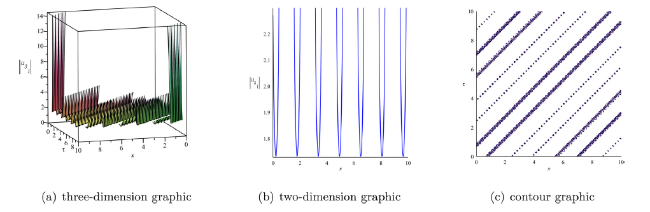
Fig. 1. The solution $\left|u_{3_{1}}(\tau, x)\right|$ of Eq. (1.1) for differential parameter. |
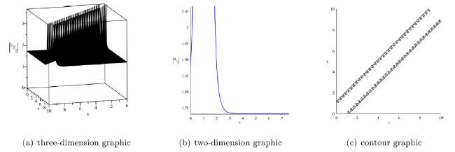
Fig. 2. The solution $\left|u_{3_{2}}(\tau, x)\right|$ of Eq. (1.1) for differential parameter. |
Remark 2.3
In the paper, we only obtain one set of traveling wave solutions of Eq. (1.1). For another set of traveling wave solutions, we can quickly obtain them by the linear transformation $Q=\rho P$ and traveling wave transformation (2.1).
3. Conclusion
In the paper, we obtain new single traveling wave solutions of the coupled Fokas-Lenells system by the complete discriminant system method of polynomials. In comparison to the other references (see Triki et al. [19], Chen et al. [37], Biswas et al. [38]), these solutions in the paper mainly include rational function solutions, implicit function solutions and Jacobian function solutions. The figures of some obtained solutions were depicted for special parameters. The corresponding three-dimensional graphic, two-dimensional graphic and two-dimensional contour graphic of traveling wave solutions are also shown in Figs. 1 and 2, respectively. We hope that the obtained results in the paper can be used to analyze the propagation of traveling wave solutions in nonlinear optical fibers and the water waves in the ocean.
Funding
This work was supported by Scientific Research Funds of Chengdu University under grant no. 2081920034.
Declaration of Competing Interest
The authors declare that they have no known competing financial interests or personal relationships that could have appeared to influence the work reported in this paper.
Acknowledgments
The authors are grateful to the anonymous reviewers for their careful reading and useful suggestions, which greatly improved the presentation of the paper.
