
1. Introduction
Thenonlinear partial differential equations(NLPDEs) are becoming more and more important in modeling the complex phenomenon involving in the fluid mechanics [1], [2], [3], optics [4], [5], [6], plasma physics [7], [8], [9], magnetic field [10], vibration [11], [12], [13], diffusion [14], [15], [16] and so on [17], [18], [19], [20], [21]. The exact solution and solitary wave solution of NLPDEs have great significance in the nonlinear theory. Some effective and powerful methods such as the sine-Gordon expansion method [22,23], extended trial equation method [24,25], variational method [26,27], generalized (G’/G) expansion method [28,29], extended rational sine-cosine and sinh-cosh method [30,31], ancient Chinese algorithm [32], extended tanh-function method [33], [34], [35], [36], [37], Exp-function method [38], [39], [40] and so on [41], [42], [43], have been developed to construct the traveling wave solutions. In this study, we will examine the unsteady korteweg-de vries model that is given as [44], [45], [46]:
$\psi_{t}+\psi \psi_{x}+\gamma \psi_{x x x}=0$
where γ is a nonzero constant. Eq. (1.1) is a general model of weak nonlinear long wave, which combines the leading order nonlinearity and dispersion to simulate the influence of deep water surface. The first term $ψ_t$ represents the time evolution of the wave propagating in one direction. The terms $ψψ_x$ and $ψ_{xxx}$ indicate the steepening and spreading of the wave respectively. Recently, the Sardar-subequation method(SSM) and the energy balance method(EBM) have received much more attention due to their effectiveness for solving the NLPDEs. So in this work, the SSM and EBM will be adopted to study Eq.(1.1). The remaining content of this paper is arranged as follows: the SSM and EBM are employed to establish the traveling wave solutions(TWSs) in Section 2. In Section 3, the behaviors of some solutions are presented in the form of the 3D plot and 2D curve. Finally, a conclusion is reached in Section 4.
2. The solutions
For seeking the TWSs, we have the following variable transformation:
$\psi(\zeta)=\psi(x, t), \zeta=x-\omega t$
Putting it into Eq.(1.1), we have:
$-\omega \psi^{\prime}+\psi \psi^{\prime}+\gamma \psi^{\prime \prime \prime}=0$
where $\psi^{\prime}=\frac{d \psi}{d \zeta}, \psi^{\prime \prime \prime}=\frac{d^{3} \psi}{d \zeta^{3}}$. Integrating Eq.(2.2) with respect to ζ once and ignoring the integral constant, we have:
$\gamma \psi^{\prime \prime}-\omega \psi+\frac{1}{2} \psi^{2}=0$
In the following content, the SSM and the EBM will be used to deal with Eq.(2.3).
2.1. The SSM
$\psi(\zeta)=\sum_{i=0} m_{i} \varphi^{i}(\zeta)$
Here $m_{i}(i=0,1,2,3 \ldots)$ is the undetermined coefficient, and there is:
$\left[\varphi^{\prime}(\zeta)\right]^{2}=\rho+a \varphi^{2}(\zeta)+\varphi^{4}(\zeta)$
where $a$ and $ρ$rare real constants. Balancing ψ″ and ψ2 in Eq.(2.3), we get $i=2$, so Eq.(2.4) can be re-expressed as:
$\psi(\zeta)=m_{0}+m_{1} \varphi(\zeta)+m_{2} \varphi^{2}(\zeta)$
Taking Eq.(2.6) into Eq.(2.3) along with Eq.(2.5), merging the same type about $φ(ζ)$ and setting their coefficients to zero yields:
$\begin{array}{l} \varphi^{0}(\zeta):-\omega m_{0}+\frac{m_{0}^{2}}{2}+2 \gamma \rho+m_{2}=0 \\ \varphi^{1}(\zeta): a \gamma m_{1}-\omega m_{1}+m_{0} m_{1}=0 \\ \varphi^{2}(\zeta): \frac{m_{1}^{2}}{2}+4 a \gamma m_{2}-\omega m_{2}+m_{0} m_{2}=0 \\ \varphi^{2}(\zeta): \frac{m_{1}^{2}}{2}+4 a \gamma m_{2}-\omega m_{2}+m_{0} m_{2}=0 \\ \varphi^{3}(\zeta): 2 \gamma m_{1}+m_{1} m_{2}=0 \\ \varphi^{4}(\zeta): 6 \gamma m_{2}+\frac{m_{2}^{2}}{2}=0 \end{array} $
Solving them, we have:
$a=\frac{\omega-m_{0}}{4 \gamma}, \rho=\frac{-2 \omega m_{0}+m_{0}^{2}}{48 \gamma^{2}} m_{1}=0 m_{2}=-12 \gamma$
So we can get the results as:
Case I: When $a=\frac{\omega-m_{0}}{4 \gamma}>0$ and $\rho=\frac{-2 \omega m_{0}+m_{0}^{2}}{48 \gamma^{2}}=0\left(m_{0}=2 \omega\right) \text {. }$ we have:
$\varphi_{1}^{ \pm}(\zeta)= \pm \sqrt{p q a} \operatorname{sech}_{p q}(\sqrt{a} \zeta)= \pm \sqrt{-\frac{p q \omega}{4 \gamma}} \operatorname{sech}_{p q}\left(\sqrt{-\frac{\omega}{4 \gamma}} \zeta\right)$
$\varphi_{2}^{ \pm}(\zeta)= \pm \sqrt{p q a} \operatorname{csch}_{p q}(\sqrt{a} \zeta)= \pm \sqrt{-\frac{p q \omega}{4 \gamma}} \operatorname{csch}_{p q}\left(\sqrt{-\frac{\omega}{4 \gamma}} \zeta\right)$
Where
$\operatorname{sech}_{p q}(\zeta)=\frac{2}{p e^{\zeta}+q e^{-\zeta}}, \operatorname{csch}_{p q}(\zeta)=\frac{2}{p e^{\zeta}-q e^{-\zeta}}$
The solutions of Eq.(1.1) are:
$\psi_{1}(x, t)=2 \omega+3 p q \omega \operatorname{sech}_{p q}^{2}\left(\sqrt{-\frac{\omega}{4 \gamma}}(x-\omega t)\right)$
$\psi_{2}(x, t)=2 \omega+3 p q \omega \operatorname{csch}_{p q}^{2}\left(\sqrt{-\frac{\omega}{4 \gamma}}(x-\omega t)\right)$
Case II: When $a=\frac{\omega-m_{0}}{4 \gamma}<0$ and $\rho=\frac{-2 \omega m_{0}+m_{0}^{2}}{48 \gamma^{2}}=0\left(m_{0}=2 \omega\right)$ we have:
$\varphi_{3}^{ \pm}(\zeta)= \pm \sqrt{-p q a \sec _{p q}}(\sqrt{-a} \zeta)= \pm \sqrt{\frac{p q \omega}{4 \gamma}} \sec _{p q}\left(\sqrt{\frac{w}{4 \gamma}} \zeta\right),$
$\varphi_{4}^{ \pm}(\zeta)= \pm \sqrt{p q a} \csc _{p q}(\sqrt{-a} \zeta)= \pm \sqrt{\frac{p q \omega}{4 \gamma}} \operatorname{csch}_{p q}\left(\sqrt{\frac{w}{4 \gamma}} \zeta\right)$
Where
$\sec _{p q}(\zeta)=\frac{2}{p e^{i \zeta}+q e^{-i \zeta}}, \csc _{p q}(\zeta)=\frac{2}{p e^{i \zeta}-q e^{-i \zeta}}$
In this case, the solutions of Eq.(1.1) can be obtained as:
$\psi_{3}(x, t)=2 \omega-3 p q \omega \sec _{p q}^{2}\left(\sqrt{\frac{\omega}{4 \gamma}}(x-\omega t)\right)$
$\psi_{4}(x, t)=2 \omega-3 p q \omega \csc _{p q}^{2}\left(\sqrt{\frac{\omega}{4 \gamma}}(x-\omega t)\right)$
Case Ⅲ: When $a=\frac{\omega-m_{0}}{4 \gamma}>0$ and $\rho=\frac{a^{2}}{4}\left(m_{0}=3 \omega \text { or } m_{0}=-\omega\right) \text {, }$ we have:
Set I: For $m_{0}=3 \omega$:
$\varphi_{5}^{ \pm}(\zeta)= \pm \sqrt{\frac{a}{2}} \tan _{p q}\left(\sqrt{\frac{a}{2}} \zeta\right)= \pm \sqrt{-\frac{\omega}{4 \gamma}} \tan _{p q}\left(\sqrt{-\frac{w}{4 \gamma}} \zeta\right),$
$\varphi_{6}^{ \pm}(\zeta)= \pm \sqrt{\frac{a}{2}} \cot _{p q}\left(\sqrt{\frac{\alpha}{2}} \zeta\right)= \pm \sqrt{-\frac{\omega}{4 \gamma}} \cot _{p q}\left(\sqrt{-\frac{\omega}{4 \gamma}} \zeta\right),$
$\begin{aligned} \varphi_{7}^{ \pm}(\zeta) & = \pm \sqrt{\frac{a}{2}}\left[\tan _{p q}(\sqrt{2 a} \zeta) \pm \sqrt{p q} \sec _{p q}(\sqrt{2 a} \zeta)\right] \\ & = \pm \sqrt{-\frac{\omega}{4 \gamma}}\left[\tan _{p q}\left(\sqrt{-\frac{\omega}{\gamma}} \zeta\right) \pm \sqrt{p q \sec _{p q}}\left(\sqrt{-\frac{\omega}{\gamma}} \zeta\right)\right] \end{aligned}$
$\begin{aligned} \varphi_{8}^{ \pm}(\zeta) & = \pm \sqrt{\frac{a}{2}}\left[\cot _{p q}(\sqrt{2 a} \zeta) \pm \sqrt{p q} \csc _{p q}(\sqrt{2 a} \zeta)\right] \\ & = \pm \sqrt{-\frac{\omega}{4 \gamma}}\left[\cot _{p q}\left(\sqrt{-\frac{\omega}{\gamma}} \zeta\right) \pm \sqrt{p q} \csc _{p q}\left(\sqrt{-\frac{\omega}{\gamma}} \zeta\right)\right] \end{aligned}$
$\begin{aligned} \varphi_{9}^{ \pm}(\zeta) & = \pm \sqrt{\frac{a}{8}}\left[\tan _{p q}\left(\sqrt{\frac{a}{8}} \zeta\right)+\cot _{p q}\left(\sqrt{\frac{a}{8}} \zeta\right)\right] \\ & = \pm \sqrt{-\frac{\omega}{16 \gamma}}\left[\tan _{p q}\left(\sqrt{-\frac{\omega}{16 \gamma}} \zeta\right) \pm \cot _{p q}\left(\sqrt{-\frac{\omega}{16 \gamma}} \zeta\right)\right] \end{aligned}$
Where
$\tan _{p q}(\zeta)=-i \frac{p e^{i \zeta}-q e^{-i \zeta}}{p e^{i \zeta}+q e^{-i \zeta}}, \cot _{p q}(\zeta)=i \frac{p e^{i \zeta}+q e^{-i \zeta}}{p e^{i \zeta}-q e^{-i \zeta}}$
So the solutions of Eq.(1.1) are got as:
$\psi_{5}(x, t)=3 \omega+3 \omega \tan _{p q}^{2}\left(\sqrt{-\frac{\omega}{4 \gamma}}(x-\omega t)\right)$
$\psi_{6}(x, t)=3 \omega+3 \omega \cot _{p q}^{2}\left(\sqrt{-\frac{\omega}{4 \gamma}}(x-\omega t)\right)$
$\begin{aligned} \psi_{7}^{ \pm}(x, t)= & 3 \omega+3 \omega\left[\tan _{p q}\left(\sqrt{-\frac{\omega}{\gamma}}(x-\omega t)\right)\right. \\ & \left. \pm \sqrt{p q} \sec _{p q}\left(\sqrt{-\frac{\omega}{\gamma}}(x-\omega t)\right)\right]^{2} \end{aligned}$
$\begin{aligned} \psi_{8}^{ \pm}(x, t)= & 3 \omega+3 \omega\left[\cot _{p q}\left(\sqrt{-\frac{\omega}{\gamma}}(x-\omega t)\right)\right. \\ & \left. \pm \sqrt{p q} \csc _{p q}\left(\sqrt{-\frac{\omega}{\gamma}}(x-\omega t)\right)\right]^{2} \end{aligned}$
$\begin{aligned} \psi_{9}^{ \pm}(x, t)= & 3 \omega+\frac{3 \omega}{4}\left[\tan _{p q}\left(\sqrt{-\frac{\omega}{16 \gamma}}(x-\omega t)\right)\right. \\ & \left. \pm \cot _{p q}\left(\sqrt{-\frac{\omega}{16 \gamma}}(x-\omega t)\right)\right]^{2} \end{aligned}$
Set II: For $m_0=−ω$:
$\varphi_{10}^{ \pm}(\zeta)= \pm \sqrt{\frac{a}{2}} \tan _{p q}\left(\sqrt{\frac{a}{2}} \zeta\right)= \pm \sqrt{\frac{\omega}{4 \gamma}} \tan _{p q}\left(\sqrt{\frac{\omega}{4 \gamma}} \zeta\right)$
$\varphi_{11}^{ \pm}(\zeta)= \pm \sqrt{\frac{a}{2}} \cot _{p q}\left(\sqrt{\frac{a}{2}} \zeta\right)= \pm \sqrt{\frac{\omega}{4 \gamma}} \cot _{p q}\left(\sqrt{\frac{\omega}{4 \gamma}} \zeta\right),$
$\begin{aligned} \varphi_{12}^{ \pm}(\zeta) & = \pm \sqrt{\frac{a}{2}}\left[\tan _{p q}(\sqrt{2 a} \zeta) \pm \sqrt{p q} \sec _{p q}(\sqrt{2 a} \zeta)\right] \\ & = \pm \sqrt{\frac{\omega}{4 \gamma}}\left[\tan _{p q}\left(\sqrt{\frac{\omega}{\gamma}} \zeta\right) \pm \sqrt{p q} \sec _{p q}\left(\sqrt{\frac{\omega}{\gamma}} \zeta\right)\right] \end{aligned}$
$\begin{aligned} \varphi_{13}^{ \pm}(\zeta) & = \pm \sqrt{\frac{a}{2}}\left[\cot _{p q}(\sqrt{2 a} \zeta) \pm \sqrt{p q} \csc _{p q}(\sqrt{2 a} \zeta)\right] \\ & = \pm \sqrt{\frac{\omega}{4 \gamma}}\left[\cot _{p q}\left(\sqrt{\frac{\omega}{\gamma}} \zeta\right) \pm \sqrt{p q} \csc _{p q}\left(\sqrt{\frac{\omega}{\gamma}} \zeta\right)\right] \end{aligned}$
$\begin{aligned} \varphi_{14}^{ \pm}(\zeta) & = \pm \sqrt{\frac{a}{8}}\left[\tan _{p q}\left(\sqrt{\frac{a}{8}} \zeta\right)+\cot _{p q}\left(\sqrt{\frac{a}{8}} \zeta\right)\right] \\ & = \pm \sqrt{\frac{\omega}{16 \gamma}}\left[\tan _{p q}\left(\sqrt{\frac{\omega}{16 \gamma}} \zeta\right) \pm \cot _{p q}\left(\sqrt{\frac{\omega}{16 \gamma}} \zeta\right)\right] \end{aligned}$
So the solutions of Eq.(1.1) are obtained as:
$\psi_{10}(x, t)=-\omega-3 \omega \tan _{p q}^{2}\left(\sqrt{\frac{\omega}{4 \gamma}}(x-\omega t)\right)$
$\psi_{11}(x, t)=-\omega-3 \omega \cot _{p q}^{2}\left(\sqrt{\frac{\omega}{4 \gamma}}(x-\omega t)\right)$
$\begin{aligned} \psi_{12}^{ \pm}(x, t)= & -\omega-3 \omega\left[\tan _{p q}\left(\sqrt{\frac{\omega}{\gamma}}(x-\omega t)\right)\right. \\ & \left. \pm \sqrt{p q \sec _{p q}}\left(\sqrt{\frac{\omega}{\gamma}}(x-\omega t)\right)\right]^{2} \end{aligned}$
$\begin{aligned} \psi_{13}^{ \pm}(x, t)= & -\omega-3 \omega\left[\cot _{p q}\left(\sqrt{\frac{\omega}{\gamma}}(x-\omega t)\right)\right. \\ & \left. \pm \sqrt{p q} \csc _{p q}\left(\sqrt{\frac{\omega}{\gamma}}(x-\omega t)\right)\right]^{2} \end{aligned}$
$\begin{aligned} \psi_{14}^{ \pm}(x, t)= & -\omega-\frac{3 \omega}{4}\left[\tan _{p q}\left(\sqrt{\frac{\omega}{16 \gamma}}(x-\omega t)\right)\right. \\ & \left. \pm \cot _{p q}\left(\sqrt{\frac{\omega}{16 \gamma}}(x-\omega t)\right)\right]^{2} \end{aligned}$
Case Ⅳ: When $a=\frac{\omega-m_{0}}{4 \gamma}<0$ and $\rho=\frac{a^{2}}{4}\left(m_{0}=3 \omega \text { or } m_{0}=-\omega\right) \text {, }$ we have:
Set I: For $m_{0}=3 \omega$:
$\varphi_{15}^{ \pm}(\zeta)= \pm \sqrt{-\frac{a}{2}} \tanh _{p q}\left(\sqrt{-\frac{a}{2}} \zeta\right)= \pm \sqrt{\frac{\omega}{4 \gamma}} \tanh _{p q}\left(\sqrt{\frac{\omega}{4 \gamma}} \zeta\right)$
$\varphi_{16}^{ \pm}(\zeta)= \pm \sqrt{-\frac{a}{2}} \operatorname{coth}_{p q}\left(\sqrt{-\frac{a}{2}} \zeta\right)= \pm \sqrt{\frac{\omega}{4 \gamma}} \operatorname{coth}_{p q}\left(\sqrt{\frac{\omega}{4 \gamma}} \zeta\right)$
$\begin{aligned} \varphi_{17}^{ \pm}(\zeta) & = \pm \sqrt{-\frac{a}{2}}\left[\tanh _{p q}(\sqrt{-2 a} \zeta) \pm \sqrt{p q} \operatorname{sech}_{p q}(\sqrt{-2 a} \zeta)\right] \\ & = \pm \sqrt{\frac{\omega}{4 \gamma}}\left[\tanh _{p q}\left(\sqrt{\frac{\omega}{\gamma}} \zeta\right) \pm \sqrt{p q} \operatorname{sech}_{p q}\left(\sqrt{\frac{\omega}{\gamma}} \zeta\right)\right] \end{aligned}$
$\begin{aligned} \varphi_{18}^{ \pm}(\zeta) & = \pm \sqrt{-\frac{a}{2}}\left[\operatorname{coth}_{p q}(\sqrt{-2 a} \zeta) \pm \sqrt{p q} \operatorname{csch}_{p q}(\sqrt{-2 a} \zeta)\right] \\ & = \pm \sqrt{\frac{\omega}{4 \gamma}}\left[\operatorname{coth}_{p q}\left(\sqrt{\frac{\omega}{\gamma}} \zeta\right) \pm \sqrt{p q} \operatorname{csch}_{p q}\left(\sqrt{\frac{\omega}{\gamma}} \zeta\right)\right] \end{aligned}$
$\begin{aligned} \varphi_{19}^{ \pm}(\zeta) & = \pm \sqrt{-\frac{a}{8}}\left[\tanh _{p q}\left(\sqrt{-\frac{a}{8}} \zeta\right)+\operatorname{coth}_{p q}\left(\sqrt{-\frac{a}{8}} \zeta\right)\right] \\ & = \pm \sqrt{\frac{\omega}{16 \gamma}}\left[\tanh _{p q}\left(\sqrt{\frac{\omega}{16 \gamma}} \zeta\right) \pm \operatorname{coth}_{p q}\left(\sqrt{\frac{\omega}{16 \gamma}} \zeta\right)\right] \end{aligned}$
Where
$\tanh _{p q}(\zeta)=\frac{p e^{\zeta}-q e^{-\zeta}}{p e^{\zeta}+q e^{-\zeta}}, \operatorname{coth}_{p q}(\zeta)=\frac{p e^{\zeta}+q e^{-\zeta}}{p e^{\zeta}-q e^{-\zeta}}$
So the solutions of Eq.(1.1) are obtained, which are:
$\psi_{15}(x, t)=3 \omega-3 \omega \tanh _{p q}^{2}\left(\sqrt{\frac{\omega}{4 \gamma}}(x-\omega t)\right)$
$\psi_{16}(x, t)=3 \omega-3 \omega \operatorname{coth}_{p q}^{2}\left(\sqrt{\frac{\omega}{4 \gamma}}(x-\omega t)\right)$
$\begin{aligned} \psi_{17}^{ \pm}(x, t)= & 3 \omega-3 \omega\left[\tanh _{p q}\left(\sqrt{\frac{\omega}{\gamma}}(x-\omega t)\right)\right. \\ & \left. \pm \sqrt{p q} \operatorname{sech}_{p q}\left(\sqrt{\frac{\omega}{\gamma}}(x-\omega t)\right)\right]^{2} \end{aligned}$
$\begin{aligned} \psi_{18}^{ \pm}(x, t)= & 3 \omega-3 \omega\left[\operatorname{coth}_{p q}\left(\sqrt{\frac{\omega}{\gamma}}(1-\omega t)\right)\right. \\ & \left. \pm \sqrt{p q} \operatorname{csch}_{p q}\left(\sqrt{\frac{\omega}{\gamma}}(1-\omega t)\right)\right]^{2} \end{aligned}$
$\begin{aligned} \psi_{19}^{ \pm}(x, t)= & 3 \omega-\frac{3}{4} \omega\left[\tanh _{p q}\left(\sqrt{\frac{\omega}{16 \gamma}}(x-\omega t)\right)\right. \\ & \left. \pm \operatorname{coth}_{p q}\left(\sqrt{\frac{\omega}{16 \gamma}}(x-\omega t)\right)\right]^{2} \end{aligned}$
Set II: For $m_{0}=-\omega$:
$\varphi_{20}^{ \pm}(\zeta)= \pm \sqrt{-\frac{a}{2}} \tanh _{p q}\left(\sqrt{-\frac{a}{2}} \zeta\right)= \pm \sqrt{-\frac{\omega}{4 \gamma}} \tanh _{p q}\left(\sqrt{-\frac{\omega}{4 \gamma}} \zeta\right)$
$\varphi_{21}^{ \pm}(\zeta)= \pm \sqrt{-\frac{a}{2}} \operatorname{coth}_{p q}\left(\sqrt{-\frac{a}{2}} \zeta\right)= \pm \sqrt{-\frac{\omega}{4 \gamma}} \operatorname{coth}_{p q}\left(\sqrt{-\frac{\omega}{4 \gamma}} \zeta\right)$
$\begin{aligned} \varphi_{22}^{ \pm}(\zeta) & = \pm \sqrt{-\frac{a}{2}}\left[\tanh _{p q}(\sqrt{-2 a} \zeta) \pm \sqrt{p q} \operatorname{sech}_{p q}(\sqrt{-2 a} \zeta)\right] \\ & = \pm \sqrt{-\frac{\omega}{4 \gamma}}\left[\tanh _{p q}\left(\sqrt{-\frac{\omega}{\gamma}} \zeta\right) \pm \sqrt{p q} \operatorname{sech}_{p q}\left(\sqrt{-\frac{\omega}{\gamma}} \zeta\right)\right] \end{aligned}$
$\begin{aligned} \varphi_{23}^{ \pm}(\zeta) & = \pm \sqrt{-\frac{a}{2}}\left[\operatorname{coth}_{p q}(\sqrt{-2 a} \zeta) \pm \sqrt{p q} \operatorname{csch}_{p q}(\sqrt{-2 a} \zeta)\right] \\ & = \pm \sqrt{-\frac{\omega}{4 \gamma}}\left[\operatorname{coth}_{p q}\left(\sqrt{-\frac{\omega}{\gamma}} \zeta\right) \pm \sqrt{p q} \operatorname{csch}_{p q}\left(\sqrt{-\frac{\omega}{\gamma}} \zeta\right)\right] \end{aligned}$
$\begin{aligned} \varphi_{24}^{ \pm}(\zeta) & = \pm \sqrt{-\frac{a}{8}}\left[\tanh _{p q}\left(\sqrt{-\frac{a}{8}} \zeta\right)+\operatorname{coth}_{p q}\left(\sqrt{-\frac{a}{8}} \zeta\right)\right] \\ & = \pm \sqrt{-\frac{\omega}{16 \gamma}}\left[\tanh _{p q}\left(\sqrt{-\frac{\omega}{16 \gamma}} \zeta\right) \pm \operatorname{coth}_{p q}\left(\sqrt{-\frac{\omega}{16 \gamma}} \zeta\right)\right] \end{aligned}$
So the solutions of Eq. (1.1) are obtained, which are:
$\psi_{20}(x, t)=-\omega+3 \omega \tanh _{p q}^{2}\left(\sqrt{-\frac{\omega}{4 \gamma}}(x-\omega t)\right)$
$\psi_{21}(x, t)=-\omega+3 \omega \operatorname{coth}_{p q}^{2}\left(\sqrt{-\frac{\omega}{4 \gamma}}(x-\omega t)\right)$
$\begin{aligned} \psi_{22}^{ \pm}(x, t)= & -\omega+3 \omega\left[\tanh _{p q}\left(\sqrt{-\frac{\omega}{\gamma}}(x-\omega t)\right)\right. \\ & \left. \pm \sqrt{p q \operatorname{sech}_{p q}}\left(\sqrt{-\frac{\omega}{\gamma}}(x-\omega t)\right)\right]^{2} \end{aligned}$
$\begin{aligned} \psi_{23}^{ \pm}(x, t)= & -\omega+3 \omega\left[\operatorname{coth}_{p q}\left(\sqrt{-\frac{\omega}{\gamma}}(x-\omega t)\right)\right. \\ & \left. \pm \sqrt{p q} \operatorname{csch}_{p q}\left(\sqrt{-\frac{\omega}{\gamma}}(x-\omega t)\right)\right] \end{aligned}$
$\begin{aligned} \psi_{24}^{ \pm}(x, t)= & -\omega+\frac{3 \omega}{4}\left[\tanh _{p q}\left(\sqrt{-\frac{\omega}{16 \gamma}}(x-\omega t)\right)\right. \\ & \left. \pm \operatorname{coth}_{p q}\left(\sqrt{-\frac{\omega}{16 \gamma}}(x-\omega t)\right)\right]^{2} \end{aligned}$
2.2. The EBM
For applying the EBM [49], we first re-write Eq.(2.3) as:
$\psi^{\prime \prime}-\frac{\omega}{\gamma} \psi+\frac{1}{2 \gamma} \psi^{2}=0$
We can establish its variational principle:
$J(\psi)=\int_{0}^{\frac{T}{4}}\left\{\frac{1}{2}\left(\frac{d \psi}{d \zeta}\right)^{2}+\frac{\omega}{2 \gamma} \psi^{2}-\frac{1}{6 \gamma} \psi^{3}\right\} d \zeta$
That is:
$\begin{aligned} J(\psi) & =\int_{0}^{\frac{T}{4}}\left\{\frac{1}{2}\left(\frac{d \psi}{d \zeta}\right)^{2}-\left[\frac{1}{6 \gamma} \psi^{3}-\frac{\omega}{2 \gamma} \psi^{2}\right]\right\} \\ d \zeta & =J(\psi)=\int_{0}^{\frac{T}{4}}\{D-S\} d \zeta \end{aligned}$
where $D$ is the kinetic energy and $S$ is potential energy respectively, there are:
$D=\frac{1}{2}\left(\frac{d \psi}{d \zeta}\right)^{2}, S=\frac{1}{6 \gamma} \psi^{3}-\frac{\omega}{2 \gamma} \psi^{2}$
Then we can get its Hamiltonian invariant:
$H=D+S=\frac{1}{2}\left(\frac{d \psi}{d \zeta}\right)^{2}+\frac{1}{b \gamma} \psi^{3}-\frac{\omega}{2 \gamma} \psi^{2}$
Now we assume Eq.(2.55) has the solution as:
$\psi(\zeta)=\Xi \cos (\Omega \zeta)$
According to the EBT, the Hamiltonian invariant should keep unchanged as:
$H=D+S=\frac{1}{2}\left(\frac{d \psi}{d \varsigma}\right)^{2}+\frac{1}{b \gamma} \psi^{3}-\frac{\omega}{2 \gamma} \psi^{2}=H_{0}$
The initial conditions of Eq.(2.59) are:
$\psi^{\prime}(0)=0, \psi(0)=\Xi$
Taking them into Eq.(2.60), we have:
$\frac{1}{6 \gamma} \Xi^{3}-\frac{\omega}{2 \gamma} \Xi^{2}=H_{0}$
Substituting Eqs.(2.61) and (2.59) into Eq.(2.60) yields:
$\begin{array}{l} \frac{1}{2}[-\Omega \Xi \sin (\Omega \zeta)]^{2}+\frac{1}{6 \gamma}[\Xi \cos (\Omega \zeta)]^{3} \\ \quad-\frac{\omega}{2 \gamma}[\Xi \cos (\Omega \zeta)]^{2}=\frac{1}{6 \gamma} \Xi^{3}-\frac{\omega}{2 \gamma} \Xi^{2} \end{array}$
By applying $\Omega \zeta=\frac{\pi}{4}$, Eq.(2.62) becomes:
$\frac{1}{4} \Omega^{2} \Xi^{2}+\frac{\sqrt{2}}{24 \gamma} \Xi^{3}-\frac{\omega \Xi^{2}}{4 \gamma}=\frac{1}{6 \gamma} \Xi^{3}-\frac{\omega}{2 \gamma} \Xi^{2}$
Which leads to:
$\Omega=\sqrt{\frac{1}{\gamma}\left(\frac{(4-\sqrt{2}) E}{6}-\omega\right)},$
Then we get the periodic solution of Eq.(1.1) as:
$\psi_{25}(x, t)=\Xi \cos \left(\sqrt{\frac{1}{\gamma}\left(\frac{(4-\sqrt{2}) \Xi}{6}-\omega\right)}(x-\omega t)\right).$
3. The numerical simulation and physical interpretation
For using $\omega=4, \gamma=-1, p=0.97, q=0.98$ is the bright solitary wave.

Fig. 1. The profile of $ψ_1$ with the parameters $\omega=4, \gamma=-1, p=0.97, q=0.98$, (a) the 3D plot, (b) the 2D curve for t=0. |
For using $\omega=4, \gamma=-1, p=0.97, q=0.98$, the performance of Eq.(2.13) is presented in Fig.2, where the solution is the singular periodic wave solution.

Fig. 2. The profile of $ψ_3$ with the parameters $\omega=4, \gamma=-1, p=0.97, q=0.98$, (a) the 3D plot, (b) the 2D curve for t=0. |
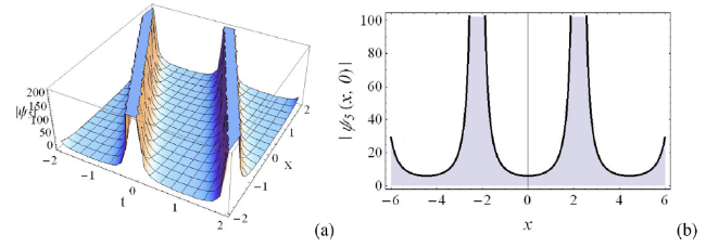
Fig. 3. The profile of $|ψ_5|$ with the parameters ω=−2, γ=1, p=0.97, q=0.98, (a) the 3D plot, (b) the 2D curve for t=0. |
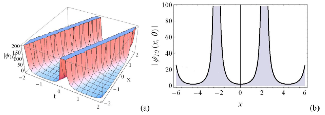
Fig. 4. The profile of $|ψ_{10}|$ with the parameters ω=2, γ=1, p=0.97, q=0.98, (a) the 3D plot, (b) the 2D curve for t=0. |
We plot the performance of $ψ_{15}$ in Fig. 5 by selecting ω=−4, γ=−1, p=0.97, q=0.98. We see that its profile is the dark solitary wave.
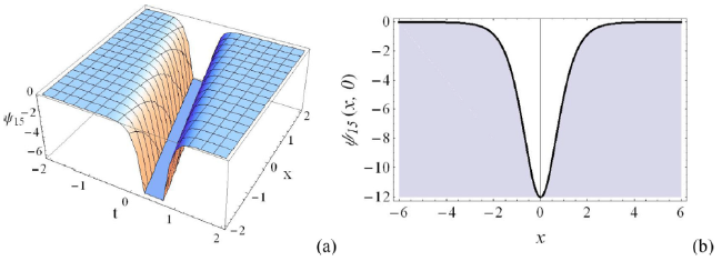
Fig. 5. The profile of $ψ_{15}$ with the parameters ω=−4, γ=−1, p=0.97, q=0.98, (a) the 3D plot, (b) the 2D curve for t=0. |
When selecting the parameters as Ξ=2 ω=−1 γ=1, the performance of the $ψ_{25}$ is drawn in Fig.6. Obviously, the solution is the perfect periodic wave solution.

Fig. 6. The profile of $ψ_{25}$ with the parameters Ξ=2, ω=−1, γ=1, (a) the 3D plot, (b) the 2D curve for t=0. |
4. Conclusion and future recommendation
This work gives a study on the unsteady korteweg-de vries equation by applying the SSM and EBM for the first time. Abundant TWSs like the bright solitary wave solutions, dark solitary wave solutions, singular periodic wave solutions and perfect periodic wave solution expressed in terms of the generalized hyperbolic functions, generalized trigonometric functions and the cosine function are constructed. The numerical simulations of the results are presented through the 3D plot and 2D curve. It is strongly proved that the proposed methods are promising tools to establish the TWSs of the PDEs arising in ocean engineering and science.
Declaration of Competing Interest
This work does not have any conflicts of interest.
Acknowledgment
This work is supported by the Key Programs of Universities in Henan Province of China (22A140006), the Fundamental Research Funds for the Universities of Henan Province (NSFRF210324), Program of Henan Polytechnic University (B2018-40), Innovative Scientists and Technicians Team of Henan Provincial High Education (21IRTSTHN016).
