
1. Introduction
The nonlinear Korteweg-De Vries (KdV) equation is a generic model for the study of weakly nonlinear long waves, incorporating leading-order nonlinearity and dispersion [1]. Boussinesq first proposed the KdV equation in 1877, and then Diederik Korteweg and Gustav de Vries rediscovered it in 1895. The KdV equation is one of useful description for modeling many physical and natural phenomena in different fields of science including shallow-water waves with weak non-linear restorative forces, ion-sound waves in plasma, acoustic waves and long internal waves in density-layered oceans on the crystal lattice, in addition to having a string equation in the Fermi-Pasta-Ulam-Tsingau problem [2]. As a result, the KdV-types problem has inspired several researchers in the study of nonlinear partial differential equations (PDEs) with different approaches developed, including Backlund transformation, symmetry groups, and the Painleve analysis methodology [3], [4]. Many researchers have also given their keen interest in developing numerical and analytical methods for finding the solution of various types of linear, nonlinear and generalised PDEs [5], [6], [7], [8], [9].
A fuzzy simulation is a good way for academics to discuss technological issues. Fuzzy set theory can be applied in various disciplines, including robotics, control systems, image processing, knowledge-based systems, power engineering, industrial automation, artificial intelligence/expert systems, consumer electronics, management, and operations research. The fractional approach to calculus has been considered as a vital support for solving sustainability and challenging phenomena in the last three decades due to its beneficial qualities such as non-locality, inheritance, high dependability, and analyticity [10], [11]. The concept of fractional with modification was created to develop a solution related to inhomogeneous equations. Various pioneer researchers have used the fractional derivative and the fractional differential equations (FDEs), including Caputo, Liouville, Letnikov, Hadamard, Riez, Abel, Caputo-Fabrizio, Grünwald, and Atangana-Baleanu [12], [13] in their discussion. FDEs can also be used to describe several important interactions in viscoelasticity, acoustics, material science, electromagnetics, and electrochemistry [14], [15], [16], [17], [18], [19].
In the fuzzy environment, several investigators have broadened the concept of derivatives to include fuzzy FDEs as a base of modelling of complex system. It allows differential equations to be written in a fuzzy framework [20]. PDEs are only sometimes the best option when dealing with real-world problems. To simulate complex behaviour, we need to collect data from many domains. These are frequently ambiguous aspects of data sets. Fuzzy PDEs have elevated the importance of current mathematical modelling due to their capacity to explain complex systems with insufficient data, attracting the slew of young authors [21]. Theory of fuzzy set [22], [23] is used in many mathematical fields such as fixed-point theory, fractional calculus, topology, integral inequality, bifurcation, control theory, image processing, artificial intelligence, operations research, and consumer electronics. Chang and Zadeh [24] suggested first about the fuzzy derivative concept, which gained popularity quickly [25]. Hukuhara’s [26] discusses the idea of differential equations with fuzzy set-valued. The fuzzy set differential equations and then fuzzy FDEs were studied using the Hukuhara derivative (HD) as a starting point. Agarwal et al. [27] used the HD idea to characterize the fuzzy Riemann-Liouville (R-L) FDEs, which laid the groundwork for the theme of fuzzy FDEs. They employed HD and the R-L differentiability notion to solve ambiguous FDEs, whereas for R-L fuzzy FDEs solution’s stability analysis is described in [28]. Allahviranloo et al. [29] constructed the fuzzy FDEs under R-L gH-differentiability with fuzzy Laplace transform. They looked at explicit solutions to unexpected FDEs under R-L gH-differentiability with Mittag-Leffler mechanisms and proved two new existence theorems for fuzzy FDEs using R-L extended gH-differentiability, and fuzzy criteria [30], [31]. Arqub et al. [32] adopted the replicating kernel technique to overcome 2-point fuzzy boundary value problems. Arqub [33] employed a variation of the replicating kernel approach for solving the fuzzy Fredholm-Volterra integrodifferential equations. Ahmad et al. [34] explored third-order fuzzy dispersive PDEs using the Caputo, Atangana-Baleanu, and Caputo-Fabrizio fractional operator frameworks. Many approaches have been adopted to solve such fuzzy FDEs but homotopy analysis method (HAM) [34], [35], is providing superior solution than other analytical and numerical approaches. To reduce the complexity while generating the solution of fuzzy fractional problem, researcher started using different transform with HAM [36], [37], [38].
The main goal of this paper is to propose a double parametric (DP) analytical approach for the nonlinear fuzzy fractional KdV equation (FFKdVE) with Caputo fractional order under the gH-differentiability, namely the q-Homotopy analysis method with Shehu transform (q-HAShTM) [39], [40]. This method is adopted to develop the parametric structure of the fuzzy mappings. It is considered an effective tool for getting solutions to the “fuzzy dispersive” and “fifth-order KdV models” under “fuzzy initial conditions”. The generic model of the “fifth-order KdV equation” describes weakly and nonlinearly interacting acoustic waves on a crystal lattice, ion-acoustic waves in plasma, shallow-water waves, and long internal waves in a density-stratified ocean. The “Shehu transform”, the integral transform, is the refinement of several existing transforms. A triangular fuzzy number (TFN) describes the “Caputo fractional derivative” (CFD) of order (0,1) in the proposed modelling problem. The “fuzzy velocity profiles” at distinct spatial positions with “crisp” and “fuzzy conditions” will be investigated using a robust DP form-based q-HASTM with its convergence analysis. Finally, the obtained results are compared with existing works to verify the efficacy and effectiveness of the proposed method.
The outline of this paper is as follows: Section 2 contains some basic notations and mathematical preliminaries about fuzzy sets and their attributes. Section 3 describes the basic solution procedure of the q-HAShTM. Section 4 discusses the uniqueness and convergence analysis of the q-HAShTM. Section 5 provides the illustrative examples to verify the efficiency and accuracy of the proposed method method. Finally, Section 6 presents the concluding remarks.
2. Mathematical preliminaries
This section covers the fundamentals of “fuzzy sets” and their properties, which can be explored in further calculations.
Definition 1
Let $\mho: \mathbb{R} \rightarrow[0,1]$ be a “fuzzy set”. Then it is knows as “fuzzy number”, if it is satisfies the subsequent property [22]
(i) ℧ is normal (for some $\wp \in \mathbb{R} ; \mho(\wp)=1 \mid$),
(ii) ℧ is upper semi continuous,
(iii) ℧ is convex, $\mho\left(\wp_{1}+(1-1) \wp_{2}\right) \geqslant(\text { for every }] \in[0,1], \wp_{1}, \wp_{2} \in \mathbb{R} \text {. }\left.\mho\left(\wp_{1}\right) \wedge \mho\left(\wp_{2}\right)\right)$
(iv) $c l\{\wp \in \mathbb{R}, \mho(\wp)>0\}$ is compact.
Definition 2
$[\mho]^{\ell}=\{\wp \in \mathbb{R}: \mho(\wp) \geqslant \ell\}$, where $\ell \in[0,1]$ and $\wp \in \mathbb{R}$.
Definition 3
(i) $\underline{\mho}(\ell)$ is non-decreasing, left continuous, bounded function over [0,1],
(ii) $\bar{\mho}(\ell)$ is a non-increasing, left continuous, bounded function over [0,1],
(iii) $\underline{\mho}(\ell) \leqslant \bar{\mho}(\ell)$.
Definition 4
For any scalar φ and $\ell \in[0,1]$. Let us assume two fuzzy numbers $\tilde{\Upsilon}_{1}=\left(\underline{\Upsilon}_{1}, \bar{\Upsilon}_{1}\right)$,$ \bar{\Upsilon}_{2}=\left(\underline{\Upsilon}_{2}, \bar{\Upsilon}_{2}\right)$. Then the addition, substitution and scalar multiplication of these fuzzy numbers can be defined as [26]: (i)
$\tilde{\Upsilon}_{1} \oplus \widetilde{\Upsilon}_{2}=\left(\underline{\Upsilon}_{1}+\underline{\Upsilon}_{2}, \bar{\Upsilon}_{1}+\bar{\Upsilon}_{2}\right)$
(ii)
$\left.\widetilde{\Upsilon}_{1} \oplus \ominus \Upsilon_{2}=\underline{\Upsilon}_{1}-\underline{\Upsilon}_{2}, \bar{\Upsilon}_{1}-\bar{\Upsilon}_{2}\right),$
(iii)
$\varphi \otimes \widetilde{\Upsilon}_{1}=\left\{\begin{array}{l} \left(\varphi \underline{\Upsilon}_{1}, \varphi \bar{\Upsilon}_{1}\right), \varphi \geqslant 0 \\ \left(\varphi \bar{\Upsilon}_{1}, \varphi \underline{\Upsilon}_{1}\right), \varphi<0 \end{array}\right.$
Definition 5Double parametric form:
Let $[\mho]^{\ell}=[\mho(\ell), \widetilde{\mho}(\ell)]$ be the parametric form of a “fuzzy number” ℧. Then the DP form in crisp conditions can be defined as,
$\underline{\mho}(\ell, \varrho)=\varrho(\bar{\mho}-\underline{\mho})+\underline{\mho}$, where ℓ and $\varrho \in[0,1]$. The deforming parameter can be represented by the embedding parameter $\varrho $ if $\varrho=0$ then $\mho(\ell, 0)=\underline{\mho}(\ell)$ (lower bound of fuzzy number) and if $\varrho=1$ then $\mho(\ell, 1)=\bar{\mho}(\ell) $ (upper bound of fuzzy number).
Definition 6
Let us consider two fuzzy numbers $\tilde{\Upsilon}_{1}=\left(\underline{\Upsilon}_{1}, \bar{\Upsilon}_{1}\right), \widetilde{\Upsilon}_{2}=\left(\underline{\Upsilon}_{2}, \bar{\Upsilon}_{2}\right)$ and $\Lambda: \widetilde{\mathbb{E}} \times \widetilde{\mathbb{E}} \rightarrow \mathbb{R}$ be a fuzzy mapping. Then Λ-distance between $\tilde{\Upsilon}_{1}$ and $\tilde{\Upsilon}_{2}$ can be defined as
$\Lambda\left(\widetilde{\Upsilon}_{1}, \widetilde{\Upsilon}_{2}\right)=\sup _{\ell \in[0,1]}\left[\max \left\{\left|\underline{\Upsilon}_{1}(\ell)-\underline{\Upsilon}_{2}(\ell)\right|,\left|\bar{\Upsilon}_{1}(\ell)-\bar{\Upsilon}_{2}(\ell)\right|\right\}\right].$
Definition 7
[29] Let F:$ \mathrm{F}:\left[b_{1}, b_{2}\right] \rightarrow \widetilde{\mathbb{\mathbb { E }}}$ is said to be continuous “fuzzy valued” mapping at point $s_0$, if for any $\epsilon>0, \exists \mid \delta>0$ such that
$\Lambda\left(\mathrm{F}(s), \mathrm{F}\left(s_{0}\right)\right)<\epsilon ; \quad \text { whenever }\left|s-s_{0}\right|<\delta$
Definition 8
[30] Let $\mathbb{k}_{1}, \mathbb{k}_{2} \in \widetilde{\mathbb{E}}$, if $\mathbb{k}_{3} \in \widetilde{\mathbb{E}}$ and $\mathbb{k}_{1}=\mathbb{k}_{2}+\mathbb{k}_{3}$. Then the H-distance $\mathbb{K}_{3}$ of $\mathbb{K}_{1}$ and $\mathbb{K}_{2}$ can be represented as $\mathbb{k}_{1} \ominus^{H} \mathfrak{k}_{2}$. But here it is observed that $\mathbb{k}_{1} \ominus^{H} \mathbb{k}_{2} \neq \mathbb{k}_{1}+(-) \mathbb{k}_{2}$.
Definition 9
A “fuzzy valued” function $\mathrm{F}:\left(a_{1}, a_{2}\right) \rightarrow \widetilde{\mathbb{E}}$ is said to be strongly generalized differential at point $s_0$ if there exist $\mathrm{F}^{\prime}\left(s_{0}\right) \in \mathbb{\mathbb { E }}$ such that [31]
(i) $\mathrm{F}^{\prime}\left(s_{0}\right)=\lim _{\varepsilon \rightarrow 0} \frac{\mathrm{F}\left(s_{0}+\varepsilon\right) \ominus^{\theta^{H}} \mathrm{~F}\left(s_{0}\right)}{\varepsilon}=\lim _{\varepsilon \rightarrow 0} \frac{\mathrm{F}\left(s_{0}\right) \ominus^{\ominus H} \mathrm{~F}\left(s_{0}-\varepsilon\right)}{\varepsilon}$,
(ii) $\mathrm{F}^{\prime}\left(s_{0}\right)=\lim _{\varepsilon \rightarrow 0} \frac{\mathrm{F}\left(s_{0}\right) \ominus^{\ominus H} \mathrm{~F}\left(s_{0}+\varepsilon\right)}{-\varepsilon}=\lim _{\varepsilon \rightarrow 0} \frac{\mathrm{F}\left(s_{0}-\varepsilon\right) \text { ® }^{{ }^{H}} \mathrm{~F}\left(s_{0}\right)}{-\varepsilon}.$
It is differentiable under the assumptions (i) and (ii) stated in the previous definition. We use the notation is (i)-differentiable and (ii)-differentiable, respectively, throughout this discussion.
Definition 10
[31] Let $\mathrm{F}(a, b) \rightarrow \mathbb{E}$ be a fuzzy valued function such that $\overline{\mathbf{F}\left(s_{0}, \ell\right)}=\left[\mathbf{F}\left(s_{0}, \ell\right), \overline{\mathbf{F}}\left(s_{0}, \ell\right)\right]$ and $\ell \in[0,1]$. Then (i) $\mathrm{F}\left(s_{0}, \ell\right)$ and $\overline{\mathrm{F}}\left(s_{0}, \ell\right)$ are differential, if F is a (1)-differential, and
$\left[\mathrm{F}^{\prime}\left(s_{0}\right)\right]^{\ell}=\left[\mathrm{F}^{\prime}\left(s_{0}, \ell\right), \overline{\mathrm{F}^{\prime}}\left(s_{0}, \ell\right)\right]$
(ii) $\mathrm{F}\left(s_{0}, \ell\right)$ and $\overline{\mathrm{F}}\left(s_{0}, \ell\right)$ are differential, if F is a (2)-differential, and
$\left[\mathrm{F}^{\prime}\left(s_{0}\right)\right]^{\ell}=\left[\overline{\mathrm{F}^{\prime}}\left(s_{0}, \ell\right), \underline{\mathbf{F}}^{\prime}\left(s_{0}, \ell\right)\right].$
Definition 11
Let us a consider fuzzy function $\tilde{\nu}_{g H}=\tilde{\nu}$ and $\tilde{\nu} \in \mathbf{C}^{F}\left[c_{1}, c_{2}\right] \cap \mathbf{L}^{F}\left[d_{1}, d_{2}\right]$. Then the “fuzzy gH-fractional Caputo’s derivatives” of $\tilde{\nu}$ is defined as
$\begin{aligned} \left({ }_{g h}^{c} \mathscr{D}^{\alpha} \tilde{\nu}\right)(\psi)= & J_{b_{1}}^{p-\alpha} \otimes(\tilde{\nu}(\psi)) \\ = & \frac{1}{\Gamma(p-\alpha)} \otimes \int_{b_{1}}^{\psi}(\psi-\varsigma)^{p-\alpha-1} \otimes \tilde{\nu}(\varsigma) \mathrm{d} \varsigma \\ & \alpha \in(p-1, p], p \in \mathbb{N}, \psi>b_{1} \end{aligned}$
As a result of the parameterized versions of $\tilde{\nu}=\left[\underline{\nu}_{\ell}(\psi), \bar{\nu}_{\ell}(\psi)\right], \| \ell \in[0,1]$ and $\psi_{0} \in\left(c_{1}, c_{2}\right)$ CFD in fuzziness is stated as
$\begin{array}{l} \left.\left[\mathscr{D}_{i-g H}^{\alpha} \underline{\nu}\right)\left(\psi_{0}\right)\right] \\ =\frac{1}{\Gamma(p-\alpha)}\left[\int_{0}^{\psi}(\psi-\varsigma)^{p-\alpha-1} \frac{d^{p}}{\mathrm{~d} \varsigma^{p}} \underline{\nu}_{i-g H}(\varsigma) \mathrm{d} \varsigma\right]_{\psi=\psi_{0}} \\ \left.\left[\mathscr{D}_{i-g H}^{\alpha} \bar{\nu}\right)\left(\psi_{0}\right)\right] \\ =\frac{1}{\Gamma(p-\alpha)}\left[\int_{0}^{\psi}(\psi-\varsigma)^{p-\alpha-1} \frac{d^{p}}{\mathrm{~d} \varsigma^{p}} \bar{\nu}_{i-g H}(\varsigma) \mathrm{d} \varsigma\right] \psi=\psi_{0} \end{array}$
Definition 12
Consider $\Lambda(s)$ is a continuous real-valued mapping, $\Lambda(s)$ such that $\Lambda(s) \neq 0$, $\forall s \in \mathbb{R}^{+}$.Also, $\tilde{\nu}$ is a real valued mapping and $e^{\varphi(s)} \otimes \tilde{\nu}(\varsigma)$ on $[0,∞)$. Then, the integral $\int_{0}^{\infty} e^{-\varphi} \otimes \tilde{v}(\zeta) \mathrm{d} \zeta$ is a “fuzzy generalized integral transform” that is expressed over a set of mappings as follows
$\mathfrak{I}=\left\{\tilde{\nu}(\varsigma): \exists \mathfrak{B}, \mathrm{k}>0,|\tilde{\nu}(\varsigma)|<\mathfrak{B} e^{(\mathrm{ks})}, i f \varsigma \geqslant 0\right\}$
as
$\mathbb{I}[\tilde{\nu}(\varsigma), s]=\mathbf{I}(s)=\Lambda(s) \int_{0}^{\infty} e^{(-\varphi(s) \varsigma)} \otimes \tilde{\nu}(\varsigma) \mathrm{d} \varsigma. \Lambda(s) \neq 0$
In Eq. (2), the assumption of a fuzzy mapping with decreasing diameter $\underline{\nu} $ and increasing diameter $\bar{v} $ was fulfilled by $\tilde{v} $.
By taking the fact of [37] and applying it to our situation, we get
$\begin{aligned} \Lambda & (s) \int_{0}^{\infty} e^{(-\varphi(s) \varsigma)} \otimes \tilde{\nu}(\varsigma) \mathrm{d} \varsigma \\ & =\left(\Lambda(s) \int_{0}^{\infty} e^{(-\varphi(s) \varsigma)} \underline{\nu}(\varsigma) \mathrm{d} \varsigma, \Lambda(s) \int_{0}^{\infty} e^{-\varphi}(s) \bar{\nu}(\varsigma) \mathrm{d} \varsigma\right) \end{aligned}$
In addition, using classical generalized integral transform [41], we get
$\mathbb{I}[\nu(\varsigma ; \ell)]=\Lambda(s) \int_{0}^{\infty} e^{(-\varphi(s) \varsigma)} \underline{\nu}(\varsigma ; \ell) \mathrm{d} \varsigma$
and
$\mathbb{I}[\bar{\nu}(\varsigma ; \ell)]=\Lambda(s) \int_{0}^{\infty} e^{(-\varphi(s) \varsigma)} \bar{\nu}(\varsigma ; \ell) \mathrm{d} \varsigma.$
Then, the expressions described above can be written a
$\Im[\tilde{\nu}(\varsigma)]=(\mathfrak{I}[\underline{\nu}(\varsigma ; \ell)], \Im[\bar{\nu}(\varsigma ; \ell)])=(\mathfrak{I}(s), \overline{\mathfrak{J}}(s)).$
Based on the ideas developed in [31], we establish the generalized fuzzy integral transform of the “generalized Hukuhara derivative” ${ }_{g H}^{c} \mathscr{D}_{S}^{\alpha} \tilde{\nu}(\varsigma)$ by Caputo.
3. A method based on theory q-HAShTM
$\mathscr{D}_{t}^{\alpha} \tilde{\nu}(\varsigma, \tau)+R \tilde{\nu}(\varsigma, \tau)+N \tilde{\nu}(\varsigma, \tau)=\tilde{f}(\varsigma, \tau)$
in which $\tilde{f}(\varsigma, \tau)$ denotes a source term, $\mathscr{D}_{t}^{\alpha} \tilde{\nu}(\varsigma, \tau)$ represents the Caputo fractional derivatives, and $R \tilde{\nu}(\varsigma, \tau)$ and $N \tilde{\nu}(\varsigma, \tau)$ are the linear and “non-linear differential operator”, respectively.
Upon expressing Eq. (7) in an interval form using the ℓ-cut technique, we have
$\begin{array}{l} {\left[\left(\mathscr{D}_{t}^{\alpha} \underline{\nu}(\varsigma, \tau, \ell), \mathscr{D}_{t}^{\alpha} \bar{\nu}(\varsigma, \tau, \ell)\right]+[R \underline{\nu}(\varsigma, \tau, \ell), R \bar{\nu}(\varsigma, \tau, \ell)]\right.} \\ \quad+[N \underline{\nu}(\varsigma, \tau, \ell), N \bar{\nu}(\varsigma, \tau, \ell)]=[\underline{f}(\varsigma, \tau, \ell), \bar{f}(\varsigma, \tau, \ell)] \end{array}$
We can write from the preceding equation using another parametric form ϱ and get
$\begin{aligned} {[\varrho} & \left.\left(\mathscr{D}_{t}^{\alpha} \bar{\nu}(\varsigma, \tau, \ell)-\mathscr{D}_{t}^{\alpha} \underline{\nu}(\varsigma, \tau, \ell)\right)+\mathscr{D}_{t}^{\alpha} \underline{\nu}(\varsigma, \tau, \ell)\right] \\ & +[\varrho(R \bar{\nu}(\varsigma, \tau, \ell)-R \underline{\nu}(\varsigma, \tau, \ell))+R \underline{\nu}(\varsigma, \tau, \ell)] \\ & +[\varrho(N \bar{\nu}(\varsigma, \tau, \ell)-N \underline{\nu}(\varsigma, \tau, \ell))+N \underline{\nu}(\varsigma, \tau, \ell)] \\ & =[\varrho(\bar{f}(\varsigma, \tau, r)-\underline{f}(\varsigma, \tau, \ell))+\underline{f}(\varsigma, \tau, \ell)]. \end{aligned}$
Here ℓ and ϱ are parameters, and ℓ,ϱ∈[0,1]. Since the above equation represents the DP form of the “fuzzy partial differential equation”. Therefore, we can write
$\varrho\left(\mathscr{D}_{t}^{\alpha} \bar{\nu}(\varsigma, \tau, \ell)-\mathscr{D}_{t}^{\alpha} \underline{\nu}(\varsigma, \tau, \ell)\right)+\mathscr{D}_{t}^{\alpha} \underline{\nu}(\varsigma, \tau, \ell)=\mathscr{D}_{t}^{\alpha} \tilde{\nu}(\varsigma, \tau, \ell, \varrho),$
$\varrho(R \bar{\nu}(\varsigma, \tau, \ell)-R \underline{\nu}(\varsigma, \tau, \ell))+R \underline{\nu}(\varsigma, \tau, \ell)=R \tilde{\nu}(\varsigma, \tau, \ell, \varrho)$
$\varrho(N \bar{\nu}(\varsigma, \tau, \ell)-N \underline{\nu}(\varsigma, \tau, \ell))+N \underline{\nu}(\varsigma, \tau, \ell)=N \tilde{\nu}(\varsigma, \tau, \ell, \varrho)$
$\varrho(\bar{f}(\varsigma, \tau, r)-\underline{f}(\varsigma, \tau, \ell))+\underline{f}(\varsigma, \tau, \ell)=\tilde{f}(\varsigma, \tau, \ell, \varrho),$
$\varrho(\bar{\nu}(\varsigma, \tau, \ell)-\underline{\nu}(\varsigma, \tau, \ell))+\underline{\nu}(\varsigma, \tau, \ell)=\tilde{\nu}(\varsigma, \tau, \ell, \varrho).$
Thus, in double parametric form, Eq. (7) can be written as.
$\mathscr{D}_{t}^{\alpha} \tilde{\nu}(\varsigma, \tau, \ell, \varrho)+R \tilde{\nu}(\varsigma, \tau, \ell, \varrho)+N \tilde{\nu}(\varsigma, \tau, \ell, \varrho)=\tilde{f}(\varsigma, \tau, \ell, \varrho)$
Applying the “Shehu transform” [40] on both sides of Eq. (15) leads to
$\begin{array}{l} \left(\frac{s}{u}\right)^{\alpha} \mathbf{S}[\tilde{\nu}(\varsigma, \tau, \ell, \varrho)]-\sum_{k=0}^{n-1}\left(\frac{s}{u}\right)^{\alpha-p-1} \tilde{\nu}^{p}(\varsigma, 0) \\ \quad+\mathbf{S}[R(\tilde{\nu}(\varsigma, \tau, \ell, \varrho)]+\mathbf{S}[N(\tilde{\nu}(\varsigma, \tau, \ell, \varrho)] \\ \quad=\mathbf{S}[\tilde{f}(\varsigma, \tau, \ell, \varrho)]. \end{array}$
Equivalently
$\begin{array}{c} \mathbf{S}[\tilde{\nu}(\varsigma, \tau, \ell, \varrho)]-\left(\frac{u}{s}\right)^{\alpha} \sum_{k=0}^{n-1}\left(\frac{s}{u}\right)^{\alpha-p-1} \tilde{\nu}^{p}(\varsigma, 0, \ell, \varrho) \\ +\left(\frac{u}{s}\right)^{\alpha} \mathbf{S}[R(\tilde{\nu}(\varsigma, \tau, \ell, \varrho)))+N(\tilde{\nu}(\varsigma, \tau, \ell, \varrho) \\ -f(\varsigma, \tau, \ell, \varrho)]=0 \end{array}$
Let us the define the nonlinear operator:
$\begin{aligned} \mathscr{N}[\widetilde{w}(\varsigma, \tau, \ell, \varrho ; q)]= & \mathbf{S}[\widetilde{w}(\varsigma, \tau, \ell, \varrho ; q)] \\ & -\left(\frac{u}{s}\right)^{\alpha} \sum_{k=0}^{n-1}\left(\frac{s}{u}\right)^{\alpha-p-1} \widetilde{W}^{p} \\ & (\varsigma, \tau, \ell, \varrho ; q)\left(0^{+}\right) \\ & +\left(\frac{u}{s}\right)^{\alpha} \mathbf{S}[R(\widetilde{w}(\varsigma, \tau, \ell, \varrho ; q) \\ & +N(\widetilde{w}(\varsigma, \tau, \ell, \varrho ; q)-\tilde{f}(\varsigma, \tau, \ell, \varrho)] \end{aligned}$
where $|\widetilde{\omega}(\varsigma, \tau, \ell, \varrho ; q)|$ represents “fuzzy-valued” function of $\mid \zeta, \tau, \ell, \varrho,q \in\left[\frac{1}{n}\right](n \geq 1)$, and q is an embedding parameter.
As a result, we construct the q-Homotopy series as follows:
$\begin{array}{l} (1-n q) \mathbf{S}\left[\widetilde{w}(\varsigma, \tau, \ell, \varrho ; q)-\tilde{\nu}_{0}(\varsigma, \tau, \ell, \varrho)\right] \\ \quad=\hbar q \widetilde{H}(\varsigma, \tau, \ell, \varrho)) \mathscr{N}[\widetilde{w}(\varsigma, \tau, r, \varrho ; q)] \end{array}$
Here the Shehu transform is represented as $\mathbf{s},|\widetilde{H}(\varsigma, \tau, \ell, \varrho)|$ is a nonzero auxiliary function, $\hbar$ is a nonzero auxiliary parameter and $\tilde{\nu}_{0}(\varsigma, \tau, \ell, \varrho)$ is the “initial guess” of $\tilde{\nu}(\varsigma, \tau, \ell, \varrho)$. The $\widetilde{w}(\varsigma, \tau, r, \varrho ; q)$ is the “unknown function”. In the cases of $q=0q=\frac{1}{n}$1n and $\widetilde{w}(\varsigma, \tau, r, \varrho ; q)$, we can obtain
$\widetilde{w}(\varsigma, \tau, r, \varrho ; 0)=\tilde{\nu}_{0}(\varsigma, \tau, \ell, \varrho), \widetilde{w}\left(\varsigma, \tau, r, \varrho ; \frac{1}{n}\right)=\tilde{\nu}(\varsigma, \tau, \ell, \varrho)$
when the value of q increases from 0 to $\frac{1}{n}$, the solution $w(\varsigma, \tau ; q)$ converges from $\left.\tilde{\nu}_{0}(\varsigma, \tau, \ell, \varrho)\right)$ to $\tilde{\nu}(\varsigma, \tau, \ell, \varrho))$. So we get
$w(\varsigma, \tau, \ell, \varrho ; q)$ by expanding the “Taylor series expansion” with respect to q as
$\widetilde{w}(\varsigma, \tau, r, \varrho ; q)=\tilde{\nu}_{0}(\varsigma, \tau, \ell, \varrho)+\sum_{m=1}^{\infty} \tilde{\nu}_{m}(\varsigma, \tau, \ell, \varrho) q^{m} $
in which $\tilde{\nu}_{m}(\varsigma, \tau, \ell, \varrho)$ stands for
$\tilde{\nu}_{m}(\varsigma, \tau, \ell, \varrho)=\left.\frac{1}{m!} \frac{\partial^{m} \tilde{w}(\varsigma, \tau, r, \varrho ; q)}{\partial q^{m}}\right|_{q=0}$
At $q=\frac{1}{n}$, the selection of the “auxiliary linear operator”, $\tilde{\nu}_{0}(\varsigma, \tau, \ell, \varrho), n, \hbar \mid$ is more appropriate than Eq. (22), against one of the solutions of the relation
$\tilde{\nu}(\varsigma, \tau)=\tilde{\nu}_{0}(\varsigma, \tau)+\sum_{m=1}^{\infty} \tilde{\nu}_{m}(\varsigma, \tau, \ell, \varrho)\left(\frac{1}{n}\right)^{m}$
Let us represent a vector $\overrightarrow{\tilde{\nu}}_{m}$ as
$\overrightarrow{\vec{\nu}}_{m}=\left\{\tilde{\nu}_{0}(\varsigma, \tau, \ell, \varrho), \tilde{\nu}_{1}(\varsigma, \tau), \tilde{\nu}_{2}(\varsigma, \tau, \ell, \varrho), \cdots, \tilde{\nu}_{m}(\varsigma, \tau, \ell, \varrho)\right\}$
Dividing Eq. (19) by m!, m-times differentiate with respect to q, and inserting q=0, the deformation equation of mth-order can be obtained as follows:
$\begin{array}{l} \mathbf{S}\left[\tilde{\nu}_{m}(\varsigma, \tau, \ell, \varrho)-\Psi_{m} \tilde{\nu}_{m-1}(\varsigma, \tau, \ell, \varrho)\right] \\ \quad=\hbar H(\varsigma, \tau, \ell, \varrho)) \Re_{\mathrm{m}}\left(\overrightarrow{\tilde{\nu}}_{m-1}\right) \end{array}$
where $\Re_{\mathrm{m}}\left(\overrightarrow{\tilde{\nu}}_{m-1}\right)$ stands for
$\mathfrak{R}_{\mathrm{m}}\left(\overrightarrow{\tilde{\nu}}_{m-1}\right)=\left.\frac{1}{(m-1)!} \frac{\partial^{m-1} \mathscr{N}[\widetilde{w}(\varsigma, \tau, r, \varrho ; q)]}{\partial q^{m-1}}\right|_{q=0}$
And
$\Psi_{m}=\left\{\begin{array}{ll} 0, & m \leq 1 \\ n, & m>1 \end{array}\right.$
Regarding the inverse “Shehu Transform” on the relation (25), we obtain
$\begin{aligned} \tilde{\nu}_{m}(\varsigma, \tau, r, \varrho)= & \Psi_{m} \tilde{\nu}_{m-1}(\varsigma, \tau, r, \varrho) \\ & +\mathbf{S}^{-1}\left[\hbar \widetilde{H}(\varsigma, \tau, r, \varrho) R_{m}\left(\vec{\nu}_{m-1}\right)\right] \end{aligned}$
Thus upon solving Eq. (27) using Eq. (26), we can get the solution:
$\tilde{\nu}(\varsigma, \tau, r, \varrho)=\sum_{m=0}^{\infty} \tilde{\nu}_{m}(\varsigma, \tau, r, \varrho)\left(\frac{1}{n}\right)^{m}$
As a result, we may identify the series solution that is always convergence using the convergence control parameter $\hbar$. The convergence analysis of the original problem Eq. (15) is the subject of the next section.
4. Convergence analysis of fuzzy fractional q-HAShTM
In this section, we study the uniqueness and convergence analysis of (15).
Theorem 1
Proof
Let us consider a nonlinear “fuzzy fractional differential” Eq. (7) whose solution can be expressed as
$\sum_{m=0}^{\infty} \tilde{\nu}(\varsigma, \tau, \ell, \varrho)=\tilde{\nu}_{0}(\varsigma, \tau, \ell, \varrho)+\sum_{m=1}^{\infty} \tilde{\nu}_{m}(\varsigma, \tau, \ell, \varrho)\left(\frac{1}{n}\right)^{m}$
Where
$\begin{array}{l} \tilde{\nu}_{m}(\varsigma, \tau, \ell, \varrho)=\left(\phi_{m}+h\right) \tilde{\nu}_{m-1}(\varsigma, \tau, \ell, \varrho) \\ \quad-\left(1-\frac{\phi}{n}\right) \hbar \mathbf{S}^{-1}\left[\left(\frac{u}{s}\right)^{\alpha} \sum_{k=0}^{n-1}\left(\frac{u}{s}\right)^{\alpha-k-1} \tilde{\nu}^{k}(\eta, \tau, \xi, \beta, 0)\right] \\ \quad+\hbar \mathbb{S}^{-1}\left[( \frac { u } { s } ) ^ { \alpha } \mathbf { S } \left[\mathscr { R } \left(\tilde{\nu}_{m-1}(\varsigma, \tau, \ell, \varrho)+T_{m-1}\right.\right.\right. \\ \left.\left.\quad+\left(1-\frac{\phi}{n}\right) \widehat{f}(\eta, \tau)\right)\right]. \end{array}$
Let $\tilde{v} $ and $\tilde{\nu} \star$ be two alternative solutions of Eq. (29). Upon using the preceding equation, it find:
$\begin{aligned} \left|\tilde{\nu}-\tilde{\nu}^{\star}\right|= & \mid(n+\hbar)\left(\tilde{\nu}-\tilde{\nu}^{\star}\right) \\ & \left.+\hbar \mathbf{S}^{-1}\left[\left(\frac{u}{s}\right)^{\alpha} \mathbf{S}\left[\mathscr{R}\left(\tilde{\nu}-\tilde{\nu}^{\star}\right)+\mathscr{N}\left(\tilde{\nu}-\tilde{\nu}^{\star}\right)\right]\right] \right\rvert\, \end{aligned}$
Upon using the “convolution theorem”,the “Shehu transform” can be obtained as follows
$\begin{aligned} \left|\tilde{\nu}-\tilde{\nu}^{\star}\right|= & (n+\hbar)\left|\left(\tilde{\nu}-\tilde{\nu}^{\star}\right)\right|+\hbar \int_{0}^{\tau}\left(\left|\mathscr{R}\left(\tilde{\nu}-\tilde{\nu}^{\star}\right)\right|\right. \\ & \left.+\left|\mathscr{N}\left(\tilde{\nu}-\tilde{\nu}^{\star}\right)\right|\right) \frac{(\tau-t)^{\alpha}}{\Gamma(1+\alpha)} \mathrm{d} t \\ & \leqslant(n+\hbar)\left|\left(\tilde{\nu}-\tilde{\nu}^{\star}\right)\right|+\hbar \int_{0}^{\tau}\left(\left|\varsigma\left(\tilde{\nu}-\tilde{\nu}^{\star}\right)\right|\right. \\ & \left.+\left|\sigma\left(\tilde{\nu}-\tilde{\nu}^{\star}\right)\right|\right) \frac{(\tau-t)^{\alpha}}{\Gamma(1+\alpha)} \mathrm{d} t \end{aligned}$
With the help of the “integral mean value theorem”, we conclude that
$\begin{aligned} \left|\tilde{\nu}-\tilde{\nu}^{\star}\right|= & (n+\hbar)\left|\left(\tilde{\nu}-\tilde{\nu}^{\star}\right)\right|+\hbar\left(\left|\varsigma\left(\tilde{\nu}-\tilde{\nu}^{\star}\right)\right|\right. \\ & \left.+\left|\sigma\left(\tilde{\nu}-\tilde{\nu}^{\star}\right)\right|\right) \kappa \leqslant\left|\tilde{\nu}-\tilde{\nu}^{\star}\right| \zeta \end{aligned}$
which gives $(1-\zeta)\left|\tilde{\nu}-\tilde{\nu}^{\star}\right| \leqslant 0$. Because $0<\zeta<1$, therefore, $|\tilde{\nu}-\tilde{\nu} \star|=0$, which implies that $\tilde{\nu}=\tilde{\nu}^{\star}$. Hence, the solution is unique. □
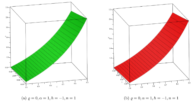
Fig. 1. Surface solution of approximate and exact with DP approach for Example 1. |
Theorem 2
Let us consider a nonlinear mapping $F: \mathbf{E} \rightarrow \mathbf{E}$, where $\mathbf{E}$ to be a Banach space and assume that
$\|F(\tilde{\tilde{\nu}})-F(\tilde{\vartheta})\| \leqslant \zeta\|\tilde{\nu}-\tilde{\vartheta}\|, \quad \forall \tilde{\nu}, \tilde{\vartheta} \in \mathbf{E}$
According to “Banach’s fixed point theory” [44, 45], F has a fixed point; besides, with a random selection of $\tilde{\nu}_{0}, \tilde{\vartheta}_{0} \in \mathbf{E},$, the sequence formed by the q-HAShTM converges to the fixed point of F and
$\left\|\tilde{\nu}_{m}-\tilde{\nu}_{k}\right\| \leqslant \frac{\zeta^{n}}{(1-\zeta)}\left\|\tilde{\nu}_{1}-\tilde{\nu}_{0}\right\|.$
Proof
Let $(C[I],\|\cdot\|)$ be a Banach space of all continuous function on I with the norm expressed as $\|g(\tau)\|=\max _{\tau \in I}|g(\tau)|$.
In the Banach space, we now show that the sequence $\tilde{\nu}_{n}$ is a Cauchy sequence.
$\begin{aligned} \left\|\tilde{\nu}_{m}-\tilde{\nu}_{k}\right\|= & \max _{\tau \in I}\left|\tilde{\nu}_{m}-\tilde{\nu}_{k}\right| \\ = & \max _{\tau \in I} \mid(n+\hbar)\left(\tilde{\nu}_{m-1}-\tilde{\nu}_{k-1}\right) \\ & \left.+\hbar \mathbb{S}^{-1}\left[\left(\frac{u}{s}\right) \alpha \mathbb{S}\left[\mathscr{R}\left(\tilde{\nu}_{m-1}-\tilde{\nu}_{k-1}\right)+\mathscr{N}\left(\tilde{\nu}_{m-1}-\tilde{\nu}_{k-1}\right)\right]\right] \right\rvert\, \\ = & \max _{\tau \in I}\left[\left|(n+\hbar)\left(\tilde{\nu}_{m-1}-\tilde{\nu}_{k-1}\right)\right|\right. \\ & +\mathbb{S}^{-1}\left[\left(\frac{u}{s}\right)^{\alpha} \mathbb{S}\left[\left|\mathscr{R}\left(\tilde{\nu}_{m-1}-\tilde{\nu}_{k-1}\right)\right|+\left|\mathscr{N}\left(\tilde{\nu}_{m-1}-\tilde{\nu}_{k-1}\right)\right|\right]\right. \end{aligned}$
Now upon using the “convolution theorem” for “Shehu transform”, we get
$\begin{aligned} \left\|\tilde{\nu}_{m}-\tilde{\nu}_{k}\right\| \leqslant & \max _{\tau \in I}|(n+\hbar)|\left(\tilde{\nu}_{m-1}-\tilde{\nu}_{k-1}\right) \mid \\ & +\hbar \int_{0}^{\tau}\left[\left|\mathscr{R}\left(\tilde{\nu}_{m-1}-\tilde{\nu}_{k-1}\right)\right|\right. \\ & \left.+\left|\mathscr{N}\left(\tilde{\nu}_{m-1}-\tilde{\nu}_{k-1}\right)\right|\right] \frac{(\tau-t)^{\alpha}}{\Gamma(1+\alpha)} d t \\ \leqslant & \max _{\tau \in I}|(n+\hbar)|\left(\tilde{\nu}_{m-1}-\tilde{\nu}_{k-1}\right) \mid \\ & +\hbar \int_{0}^{\tau}\left[\varsigma\left|\left(\tilde{\nu}_{m-1}-\tilde{\nu}_{k-1}\right)\right|\right. \\ & \left.+\sigma\left|\left(\tilde{\nu}_{m-1}-\tilde{\nu}_{k-1}\right)\right|\right] \frac{(\tau-t)^{\alpha}}{\Gamma(1+\alpha)} \mathrm{d} t \end{aligned}$
Upon applying the “integral mean value theorem” [Theorem 1] leads to
$\begin{aligned} \left\|\tilde{\nu}_{m}-\tilde{\nu}_{k}\right\| \leqslant & \max _{\tau \in I}\left[|(n+\hbar)|\left(\tilde{\nu}_{m-1}-\tilde{\nu}_{k-1}\right) \mid\right. \\ & \left.+\hbar\left(\varsigma\left|\tilde{\nu}_{m-1}-\tilde{\nu}_{k-1}\right|+\sigma\left|\tilde{\nu}_{m-1}-\tilde{\nu}_{k-1}\right|\right) \kappa\right] \\ \leqslant & \zeta\left\|\tilde{\nu}_{m-1}-\tilde{\nu}_{k-1}\right\|. \end{aligned}$
Setting m=k+1, we have
$\begin{aligned} \left\|\tilde{\nu}_{k+1}-\tilde{\nu}_{k}\right\| & \leqslant \zeta\left\|\tilde{\nu}_{k}-\tilde{\nu}_{k-1}\right\| \leqslant \zeta^{2}\left\|\tilde{\nu}_{k-1}-\tilde{\nu}_{k-2}\right\| \\ & \leqslant \cdots \leqslant \zeta^{k}\left\|\tilde{\nu}_{1}-\tilde{\nu}_{0}\right\| \end{aligned}$
By “triangle inequality”, it obtain
$\begin{aligned} \| \tilde{\nu}_{m} & -\tilde{\nu}_{k} \| \\ & \leqslant\left\|\tilde{\nu}_{k+1}-\tilde{\nu}_{k-1}\right\|+\left\|\tilde{\nu}_{k+2}-\tilde{\nu}_{k+1}\right\|+\cdots+\left\|\tilde{\nu}_{m}-\tilde{\nu}_{m-1}\right\| \\ & \leqslant\left[\zeta^{k}+\zeta^{k+1}+\zeta^{k+2}+\cdots+\zeta_{m-1}\right]\left\|\tilde{\nu}_{1}-\tilde{\nu}_{0}\right\| \\ & \leqslant \zeta^{k}\left[1+\zeta+\zeta^{2}+\cdots+\zeta^{m-1-k}\right]\left\|\tilde{\nu}_{1}-\tilde{\nu}_{0}\right\| \\ & \leqslant \zeta^{k}\left[\frac{1-\zeta^{m-1-k}}{1-\zeta}\right]\left\|\tilde{\nu}_{1}-\tilde{\nu}_{0}\right\| \end{aligned}$
Since 0<ζ<1, so $1-\zeta^{m-1-k}<1$, then we obtain
$\left\|\tilde{\nu}_{m}-\tilde{\nu}_{k}\right\| \leqslant \frac{\zeta^{k}}{(1-\zeta)}\left\|\tilde{\nu}_{1}-\tilde{\nu}_{0}\right\|$
Since $\left\|\tilde{\nu}_{1}-\tilde{\nu}_{0}\right\|<\infty$, and as m→∞ it implies $\left\|\tilde{\nu}_{m}-\tilde{\nu}_{n}\right\|<\infty$. Thus, the sequence ν˜n is a Cauchy sequence in C[I], and is convergent. □
Theorem 3
Let $\tilde{\nu}(\varsigma, \tau, \ell, \varrho)$ be an approximate analytical solution of the series $\sum_{m=0}^{k} \tilde{\nu}_{m}(\varsigma, \tau, \ell, \varrho)\left(\frac{1}{n}\right)^{k}$. For every $k \in \mathbb{N}, \exists \beta \in(0,1)$ and $\beta=\frac{\zeta}{n}$, where $\zeta \in(0,1)$ such that $\left\|\tilde{\nu}_{m+1}(\varsigma, \tau, \ell, \varrho)\right\| \leqslant \zeta\left\|\tilde{\nu}_{m}(\varsigma, \tau, \ell, \varrho)\right\|$, then we obtain the “maximum error” as
$\left\|\tilde{\nu}(\varsigma, \tau, \ell, \varrho)-\sum_{m=0}^{k} \tilde{\nu}_{m}(\varsigma, \tau, \ell, \varrho)\left(\frac{1}{n}\right)^{k}\right\| \leqslant \frac{\beta^{k+1}}{1-\beta}\left\|\tilde{\nu}_{0}(\varsigma, \tau, \ell, \varrho)\right\|.$
Proof
Due to $ \tilde{\nu}(\varsigma, \tau, \ell, \varrho) $ is an approximate analytical solution of the series $ \sum_{m=0}^{k} \tilde{\nu}_{m}(\varsigma, \tau, \ell, \varrho)\left(\frac{1}{n}\right)^{k} $, we can write
$ \begin{array}{l} \left\|\tilde{\nu}(\varsigma, \tau, \ell, \varrho)-\sum_{m=0}^{k} \tilde{\nu}_{m}(\varsigma, \tau, \ell, \varrho)\left(\frac{1}{n}\right)^{k}\right\| \\ =\left\|\sum_{m=k+1}^{\infty} \tilde{\nu}_{m}(\varsigma, \tau, \ell, \varrho)\left(\frac{1}{n}\right)^{k}\right\| \\ \leqslant \sum_{m=k+1}^{\infty}\left\|\tilde{\nu}_{m}(\varsigma, \tau, \ell, \varrho)\right\|\left(\frac{1}{n}\right)^{k} \\ \leqslant \sum_{m=k+1}^{\infty} \beta^{m}\left\|\tilde{\nu}_{0}(\varsigma, \tau, \ell, \varrho)\right\| \frac{1}{n^{k}} \\ \leqslant \beta^{k+1}\left(1+\beta+\beta^{2}+\beta^{3}+\ldots\right)\left\|\tilde{\nu}_{0}(\varsigma, \tau, \ell, \varrho)\right\| \\ \leqslant \frac{\beta^{k+1}}{1-\beta}\left\|\tilde{\nu}_{0}(\varsigma, \tau, \ell, \varrho)\right\| \end{array} $
which proves the theorem. □
5. Numerical results and discussion
In this section, we apply the “fuzzy DP approach” and the q-HAShTM for several test problems.
Example 1
Let us consider a fifth-order nonlinear FFKdVE:
$ \begin{aligned} \mathbf{D}_{\tau}^{\alpha} \tilde{\nu}(\varsigma, \tau)= & 20 \otimes \tilde{\nu}^{2}(\varsigma, \tau) \otimes \frac{\partial^{3} \tilde{\nu}(\varsigma, \tau)}{\partial \varsigma^{3}} \ominus \frac{\partial^{5} \tilde{\nu}(\varsigma, \tau)}{\partial \varsigma^{5}} \\ & \ominus \frac{\partial \tilde{\nu}(\varsigma, \tau)}{\partial \varsigma} \otimes \frac{\partial^{2} \tilde{\nu}(\varsigma, \tau)}{\partial \varsigma^{2}} \ominus \tilde{\nu}^{2}(\varsigma, \tau) \\ & \otimes \frac{\partial^{2} \tilde{\nu}(\varsigma, \tau)}{\partial \varsigma^{2}} \ominus \frac{\partial \tilde{\nu}(\varsigma, \tau)}{\partial \varsigma} \end{aligned} $
with fuzzy initial condition (IC)
$ \tilde{\nu}(\varsigma, 0)=\frac{\tilde{B}}{\varsigma} $
where $ \widetilde{B}=[-1,0,1] $ is an TFN. It can also expressed in ℓ-cut i.e.$ [\underline{B}, \bar{B}]=[\ell-1,1-\ell] $.
With the help of Eqs. (8) to (14), Eqs. (33) and (34) can be restated in DP form as:
$ \begin{aligned} \mathbf{D}_{\tau}^{\alpha} \tilde{\nu}(\varsigma, \tau, \ell, \varrho)= & 20 \tilde{\nu}^{2}(\varsigma, \tau) \frac{\partial^{3} \tilde{\nu}(\varsigma, \tau, \ell, \varrho)}{\partial \varsigma^{3}}-\frac{\partial^{5} \tilde{\nu}(\varsigma, \tau, \ell, \varrho)}{\partial \varsigma^{5}} \\ & -\frac{\partial \tilde{\nu}(\varsigma, \tau, \ell, \varrho)}{\partial \varsigma} \frac{\partial^{2} \tilde{\nu}(\varsigma, \tau, \ell, \varrho)}{\partial \varsigma^{2}} \\ & -\tilde{\nu}^{2}(\varsigma, \tau, \ell, \varrho) \frac{\partial^{2} \tilde{\nu}(\varsigma, \tau, \ell, \varrho)}{\partial \varsigma^{2}}-\frac{\partial \tilde{\nu}(\varsigma, \tau, \ell, \varrho)}{\partial \varsigma} \end{aligned} $
and
$ \widetilde{E}(\ell, \varrho)=\varrho\{\bar{B}-\underline{B}\}+\underline{B}=\varrho\{(2-\ell)\}+1-\ell. $
Now let us write the fuzzy IC in DP form as
$ \tilde{\nu}(\varsigma, 0, \ell, \varrho)=\frac{\tilde{E}(\ell, \varrho)}{\varsigma} $
We get Eq. (35) by performing the “Shehu transform” and using the IC’s on Eq. (36) as
$ \begin{aligned} \mathscr{S}[\tilde{\nu}(\varsigma, \tau, \ell, \varrho)] & -\frac{u}{s}\left(\frac{\widetilde{E}(\ell, \varrho)}{\varsigma}\right) \\ & +\frac{u^{\alpha}}{s^{\alpha}} \mathscr{S}\left[-20 \tilde{\nu}^{2}(\varsigma, \tau) \frac{\partial^{3} \tilde{\nu}(\varsigma, \tau, \ell, \varrho)}{\partial \varsigma^{3}}\right. \\ & +\frac{\partial^{5} \tilde{\nu}(\varsigma, \tau, \ell, \varrho)}{\partial \varsigma^{5}}+\frac{\partial \tilde{\nu}(\varsigma, \tau, \ell, \varrho)}{\partial \varsigma} \frac{\partial^{2} \tilde{\nu}(\varsigma, \tau, \ell, \varrho)}{\partial \varsigma^{2}} \\ & \left.+\tilde{\nu}^{2}(\varsigma, \tau, \ell, \varrho) \frac{\partial^{2} \tilde{\nu}(\varsigma, \tau, \ell, \varrho)}{\partial \varsigma^{2}}+\frac{\partial \tilde{\nu}(\varsigma, \tau, \ell, \varrho)}{\partial \varsigma}\right]. \end{aligned} $
Using the proposed method, the “non-linear operator” $ \mathscr{N} $ can be defined as follows:
$ \begin{aligned} \mathscr{N} & {[\widetilde{w}(\varsigma, \tau, \ell, \varrho: q)]=\mathscr{S}[\widetilde{w}(\varsigma, \tau, \ell, \varrho ; q)]-\frac{u}{s}\left(\frac{\widetilde{E}(\ell, \varrho)}{\varsigma}\right) } \\ & +\frac{u^{\alpha}}{s^{\alpha}} \mathscr{S}\left[-20 \widetilde{w}^{2}(\varsigma, \tau, \ell, \varrho: q) \frac{\partial^{3} \widetilde{w}(\varsigma, \tau, \ell, \varrho: q)}{\partial \varsigma^{3}}\right. \\ & +\frac{\partial^{5} \widetilde{w}(\varsigma, \tau, \ell, \varrho: q)}{\partial \varsigma^{5}}+\frac{\partial \widetilde{w}(\varsigma, \tau, \ell, \varrho: q)}{\partial \varsigma} \frac{\partial^{2} \widetilde{w}(\varsigma, \tau, \ell, \varrho: q)}{\partial \varsigma^{2}} \\ & \left.+\widetilde{w}^{2}(\varsigma, \tau, \ell, \varrho: q) \frac{\partial^{2} \widetilde{w}(\varsigma, \tau, \ell, \varrho: q)}{\partial \varsigma^{2}}+\frac{\partial \widetilde{w}(\varsigma, \tau, \ell, \varrho: q)}{\partial \varsigma}\right]. \end{aligned} $
Based on the “q-FHAShTM” approach described above, the “deformation equation” of m-th order at $ \widetilde{H}(\varsigma, \tau)=1 $ can be obtained as
$ \mathbf{S}\left[\tilde{\nu}_{m}(\varsigma, \tau, \ell, \varrho)-\Psi_{m} \tilde{\nu}_{m-1}(\varsigma, \tau, \ell, \varrho)\right]=\hbar \Re_{\mathrm{m}}\left(\overrightarrow{\tilde{\nu}}_{m-1}(\varsigma, \tau, \ell, \varrho)\right), $
where
$ \begin{aligned} \Re_{\mathfrak{m}}\left(\overrightarrow{\tilde{\nu}}_{m-1}\right)= & \mathbf{S}\left[\tilde{\nu}_{m-1}\right]-\left(1-\frac{\Psi_{m}}{n}\right) \frac{u}{s}\left(\frac{\widetilde{E}(\ell, \varrho)}{\varsigma}\right) \\ & +\frac{u^{\alpha}}{s^{\alpha}} \mathbf{S}\left[-20 \sum_{i=0}^{m-1}\left(\sum_{j=0}^{i} \tilde{\nu}_{j} \tilde{\nu}_{i-j}\right) \frac{\partial^{3} \tilde{\nu}_{m-i-1}}{\partial \varsigma^{3}}\right. \\ & +\frac{\partial^{5} \tilde{\nu}_{m-1}}{\partial \varsigma^{5}}+\sum_{i=0}^{m-1} \frac{\partial \tilde{\nu}_{m-1}}{\partial \varsigma} \frac{\partial^{2} \tilde{\nu}_{i-m-1}}{\partial \varsigma^{2}} \\ & \left.+\sum_{i=0}^{m-1}\left(\sum_{j=0}^{i} \tilde{\nu}_{j} \tilde{\nu}_{i-j}\right) \frac{\partial^{2} \tilde{\nu}_{m-1-i}}{\partial \varsigma^{2}}+\frac{\partial \tilde{\nu}_{m-1}}{\partial \varsigma}\right] \end{aligned} $
Upon applying the inverse “Shehu transform” to both sides of Eq. (39), we arrive at
$ \begin{aligned} \tilde{\nu}_{m}(\varsigma, \tau, \ell, \varrho)= & \Psi_{m} \tilde{\nu}_{m-1}(\varsigma, \tau, \ell, \varrho) \\ & +\mathbf{S}^{-1}\left[\hbar \Re_{m}\left(\overrightarrow{\vec{\nu}}_{m-1}\right)(\varsigma, \tau, \ell, \varrho)\right]. \end{aligned} $
Finally, by solving the aforesaid equation systematically, we have
$ \tilde{\nu}_{0}(\varsigma, \tau, \ell, \varrho)=\frac{\tilde{E}(\ell, \varrho)}{\varsigma} $
$ \begin{aligned} \tilde{\nu}_{1}(\varsigma, \tau, \ell, \varrho)=\frac{h \tau^{\alpha}}{\Gamma(\alpha+1)}(- & \frac{120 \widetilde{E}(\ell, \varrho)}{\varsigma^{6}}-\frac{\widetilde{E}(\ell, \varrho)}{\varsigma^{2}}+\frac{120 \widetilde{E}^{3}(\ell, \varrho)}{\varsigma^{6}} \\ & \left.-\frac{2 \widetilde{E}^{2}(\ell, \varrho)}{\varsigma^{5}}+\frac{2 \widetilde{E}^{3}(\ell, \varrho)}{\varsigma^{5}}\right) \end{aligned} $
$ \begin{aligned} \tilde{\nu}_{2}(\varsigma, \tau, \ell, \varrho) \\ = \frac{(h+n) h \tau^{\alpha}}{\Gamma(\alpha+1)}\left(-\frac{120 \widetilde{E}(\ell, \varrho)}{\varsigma^{6}}-\frac{\widetilde{E}(\ell, \varrho)}{\varsigma^{2}}+\frac{120 \widetilde{E}^{3}(\ell, \varrho)}{\varsigma^{6}}\right. \\ \left.-\frac{2 \widetilde{E}^{2}(\ell, \varrho)}{\varsigma^{5}}+\frac{2 \widetilde{E}^{3}(\ell, \varrho)}{\varsigma^{5}}\right) \\ - \frac{20 \widetilde{E}^{2}(\ell, \varrho) h^{2} \tau^{2 \alpha}}{\Gamma(2 \alpha+1)}\left(\frac{362800 \widetilde{E}(\ell, \varrho)}{\varsigma^{11}}+\frac{720 \widetilde{E}(\ell, \varrho)}{\varsigma^{7}}\right. \\ \left.-\frac{3628800 \widetilde{E}^{3}(\ell, \varrho)}{\varsigma^{11}}+\frac{30240 \widetilde{E}^{2}(\ell, \varrho)}{\varsigma^{10}}-\frac{30240 \widetilde{E}^{3}(\ell, \varrho)}{\varsigma^{10}}\right) \\ + \frac{h^{2} \tau^{2 \alpha}}{\Gamma(2 \alpha+1)}\left(\frac{720 \widetilde{E}(\ell, \varrho)}{\varsigma^{7}}+\frac{2 \widetilde{E}(\ell, \varrho)}{\varsigma^{3}}-\frac{720 \widetilde{E}^{3}(\ell, \varrho)}{\varsigma^{7}}\right. \\ \left.+\frac{10 \widetilde{E}^{2}(\ell, \varrho)}{\varsigma^{6}}-\frac{10 \widetilde{E}^{3}(\ell, \varrho)}{\varsigma^{6}}\right) \\ - \frac{20 \widetilde{E}^{2}(\ell, \varrho) h^{2} \tau^{2 \alpha}}{\varsigma^{2} \Gamma(2 \alpha+1)}\left(\frac{40320 \widetilde{E}(\ell, \varrho)}{\varsigma^{9}}+\frac{24 \widetilde{E}(\ell, \varrho)}{\varsigma^{5}}\right. \\ \left.-\frac{40320 \widetilde{E}^{3}(\ell, \varrho)}{\varsigma^{9}}+\frac{420 \widetilde{E}^{2}(\ell, \varrho)}{\varsigma^{8}}-\frac{420 \widetilde{E}^{3}(\ell, \varrho)}{\varsigma^{8}}\right) \\ + \frac{240 h^{2} \widetilde{E}^{2}(\ell, \varrho) \tau^{2 \alpha}}{\varsigma^{5} \Gamma(2 \alpha+1)}\left(-\frac{120 \widetilde{E}(\ell, \varrho)}{\varsigma^{6}}-\frac{\widetilde{E}(\ell, \varrho)}{\varsigma^{2}}+\frac{120 \widetilde{E}^{3}(\ell, \varrho)}{\varsigma^{6}}\right. \\ \left.-\frac{2 \widetilde{E}^{2}(\ell, \varrho)}{\varsigma^{5}}+\frac{2 \widetilde{E}^{3}(\ell, \varrho)}{\varsigma^{5}}\right) \\ + \frac{2 h^{2} \widetilde{E}(\ell, \varrho) \tau^{2 \alpha}}{\varsigma^{3} \Gamma(2 \alpha+1)}\left(\frac{720 \widetilde{E}(\ell, \varrho)}{\varsigma^{7}}+\frac{2 \widetilde{E}(\ell, \varrho)}{\varsigma^{3}}-\frac{720 \widetilde{E}^{3}(\ell, \varrho)}{\varsigma^{7}}\right. \\ \left.+\frac{10 \widetilde{E}^{2}(\ell, \varrho)}{\varsigma^{6}}-\frac{10 \widetilde{E}^{3}(\ell, \varrho)}{\varsigma^{6}}\right) \\ + \frac{h^{2} \widetilde{E}(\ell, \varrho) \tau^{2 \alpha}}{\varsigma^{2} \Gamma(2 \alpha+1)}\left(-\frac{5040 \widetilde{E}(\ell, \varrho)}{\varsigma^{8}}-\frac{6 \widetilde{E}(\ell, \varrho)}{\varsigma^{4}}+\frac{5040 \widetilde{E}^{3}(\ell, \varrho)}{\varsigma^{8}}\right. \\ \left.-\frac{60 \widetilde{E}^{2}(\ell, \varrho)}{\varsigma^{7}}-\frac{60 \widetilde{E}^{3}(\ell, \varrho)}{\varsigma^{7}}\right) \\ + \frac{h^{2} \widetilde{E}^{2}(\ell, \varrho) \tau^{2 \alpha}}{\varsigma^{2} \Gamma(2 \alpha+1)}\left(-\frac{5040 \widetilde{E}(\ell, \varrho)}{\varsigma^{8}}-\frac{6 \widetilde{E}(\ell, \varrho)}{\varsigma^{4}}+\frac{5040 \widetilde{E}^{3}(\ell, \varrho)}{\varsigma^{8}}\right. \\ \left.-\frac{60 \widetilde{E}^{2}(\ell, \varrho)}{\varsigma^{7}}-\frac{60 \widetilde{E}^{3}(\ell, \varrho)}{\varsigma^{7}}\right) \\ + \frac{4 h^{2} \widetilde{E}^{2}(\ell, \varrho) \tau^{2 \alpha}}{\varsigma^{4} \Gamma(\alpha+1)}\left(-\frac{120 \widetilde{E}(\ell, \varrho)}{\varsigma^{6}}-\frac{\widetilde{E}(\ell, \varrho)}{\varsigma^{2}}+\frac{120 \widetilde{E}^{3}(\ell, \varrho)}{\varsigma^{6}}\right. \\ \left.-\frac{2 \widetilde{E}^{2}(\ell, \varrho)}{\varsigma^{5}}+\frac{2 \widetilde{E}^{3}(\ell, \varrho)}{\varsigma^{5}}\right) \end{aligned} $
Hence the approximate analytical solution of Eq. (35) can be expressed as
$ \begin{aligned} \tilde{\nu}(\varsigma, \tau, \ell, \varrho)= & \tilde{\nu}_{0}(\varsigma, \tau, \ell, \varrho)+\frac{\tilde{\nu}_{1}(x, t, r, \varrho)}{n}+\frac{\tilde{\nu}_{2}(x, t, r, \varrho)}{n^{2}} \\ & +\frac{\tilde{\nu}_{3}(x, t, r, \varrho)}{n^{3}}+\ldots \end{aligned} $
Thus, we have
$ \begin{array}{l} \begin{array}{l} \tilde{\nu}(\varsigma, \tau, \ell, \varrho)=\frac{\widetilde{E}(\ell, \varrho)}{\varsigma} \\ +\frac{h \tau^{\alpha}}{n \Gamma(\alpha+1)}\left(-\frac{120 \widetilde{E}(\ell, \varrho)}{\varsigma^{6}}-\frac{\widetilde{E}(\ell, \varrho)}{\varsigma^{2}}+\frac{120 \widetilde{E}^{3}(\ell, \varrho)}{\varsigma^{6}}\right. \\ \left.-\frac{2 \widetilde{E}^{2}(\ell, \varrho)}{\varsigma^{5}}+\frac{2 \widetilde{E}^{3}(\ell, \varrho)}{\varsigma^{5}}\right) \\ +\frac{1}{n^{2}}\left\{\frac { ( h + n ) h \tau ^ { \alpha } } { \Gamma ( \alpha + 1 ) } \left(-\frac{120 \widetilde{E}(\ell, \varrho)}{\varsigma^{6}}-\frac{\widetilde{E}(\ell, \varrho)}{\varsigma^{2}}+\frac{120 \widetilde{E}^{3}(\ell, \varrho)}{\varsigma^{6}}\right.\right. \\ \left.\left.-\frac{2 \widetilde{E}^{2}(\ell, \varrho)}{\varsigma^{5}}+\frac{2 \widetilde{E}^{3}(\ell, \varrho)}{\varsigma^{5}}\right)+\ldots\right\}. \end{array}\\ \tilde{\nu}(\varsigma, \tau, \ell, \varrho)=\frac{\widetilde{E}(\ell, \varrho)}{\varsigma}\\ +\frac{h \tau^{\alpha}}{n \Gamma(\alpha+1)}\left(-\frac{120 \widetilde{E}(\ell, \varrho)}{\varsigma^{6}}-\frac{\widetilde{E}(\ell, \varrho)}{\varsigma^{2}}+\frac{120 \widetilde{E}^{3}(\ell, \varrho)}{\varsigma^{6}}\right.\\ \left.-\frac{2 \widetilde{E}^{2}(\ell, \varrho)}{\varsigma^{5}}+\frac{2 \widetilde{E}^{3}(\ell, \varrho)}{\varsigma^{5}}\right)\\ +\frac{1}{n^{2}}\left\{\frac { ( h + n ) h \tau ^ { \alpha } } { \Gamma ( \alpha + 1 ) } \left(-\frac{120 \widetilde{E}(\ell, \varrho)}{\varsigma^{6}}-\frac{\widetilde{E}(\ell, \varrho)}{\varsigma^{2}}+\frac{120 \widetilde{E}^{3}(\ell, \varrho)}{\varsigma^{6}}\right.\right.\\ \left.\left.-\frac{2 \widetilde{E}^{2}(\ell, \varrho)}{\varsigma^{5}}+\frac{2 \widetilde{E}^{3}(\ell, \varrho)}{\varsigma^{5}}\right)+\ldots\right\}. \end{array} $
By Virtue of Definition 5 in Eq. (45), and by putting $v$, i.e., lower bound solution, we obtain
$ \begin{aligned} \tilde{\nu}(\varsigma, \tau, \ell, \varrho)= & \tilde{\nu}(\varsigma, \tau, 0)=[\tilde{\nu}(\varsigma, \tau)]^{\ell}=\underline{\nu}(\varsigma, \tau, \ell), \\ \underline{\nu}(\varsigma, \tau, \ell)= & \frac{\underline{E}(\ell)}{\varsigma} \\ & +\frac{h \tau^{\alpha}}{n \Gamma(\alpha+1)}\left(-\frac{120 \underline{E}(\ell)}{\varsigma^{6}}-\frac{\underline{E}(\ell)}{\varsigma^{2}}+\frac{120 \underline{E}^{3}(\ell)}{\varsigma^{6}}\right. \\ & \left.\quad-\frac{2 \underline{E^{2}(\ell)}}{\varsigma^{5}}+\frac{2 \underline{E^{3}(\ell)}}{\varsigma^{5}}\right) \\ & +\frac{1}{n^{2}}\left\{\frac { ( h + n ) h \tau ^ { \alpha } } { \Gamma ( \alpha + 1 ) } \left(-\frac{120 \underline{E}(\ell)}{\varsigma^{6}}-\frac{\underline{E}(\ell)}{\varsigma^{2}}+\frac{120 \underline{E}^{3}(\ell)}{\varsigma^{6}}\right.\right. \\ & \left.\left.-\frac{2 \underline{E}^{2}(\ell)}{\varsigma^{5}}+\frac{2 \underline{E}^{3}(\ell)}{\varsigma^{5}}\right)+\ldots\right\}. \end{aligned} $
In a similar way, using Definition 5 in Eq. (45), and putting $ \varrho=1 $, i.e., lower bound solution and $ \widetilde{E}(\ell, 0)=\underline{E}(\ell) $, we get
$ \begin{aligned} \tilde{\nu}(\varsigma, \tau, \ell, \varrho)= & \tilde{\nu}(\varsigma, \tau, 1)=[\tilde{\nu}(\varsigma, \tau)]^{\ell}=\bar{\nu}(\varsigma, \tau, \ell) \\ \bar{\nu}(\varsigma, \tau, \ell)= & \frac{\bar{E}(\ell)}{\varsigma} \\ & +\frac{h \tau^{\alpha}}{n \Gamma(\alpha+1)}\left(-\frac{120 \bar{E}(\ell)}{\varsigma^{6}}-\frac{\bar{E}(\ell)}{\varsigma^{2}}+\frac{120 \bar{E}^{3}(\ell, \varrho)}{\varsigma^{6}}\right. \\ & \left.\quad-\frac{2 \bar{E}^{2}(\ell)}{\varsigma^{5}}+\frac{2 \bar{E}^{3}(\ell)}{\varsigma^{5}}\right) \\ & +\frac{1}{n^{2}}\left\{\frac { ( h + n ) h \tau ^ { \alpha } } { \Gamma ( \alpha + 1 ) } \left(-\frac{120 \bar{E}(\ell, \varrho)}{\varsigma^{6}}-\frac{\bar{E}(\ell)}{\varsigma^{2}}+\frac{120 \bar{E}^{3}(\ell)}{\varsigma^{6}}\right.\right. \\ & \left.\left.-\frac{2 \bar{E}^{2}(\ell)}{\varsigma^{5}}+\frac{2 \bar{E}^{3}(\ell)}{\varsigma^{5}}\right)+\ldots\right\} \end{aligned} $
We report the obtained results in Table 1 and Fig. 2, Fig. 3, Fig. 4 for distinct values α, ℓ and ϱ. Table 1 represents the comparative study of exact and approximate solution for q-HAShTM for distinct values of τ and ς and for fixed values of ℓ=0 and ϱ=1 (i.e, crisp case). The values of numerical results of several grid points obtained by the q-HAShTM are compared with the values of the exact solution with high precision upto the second term approximation. Fig. 2 displays the approximate and the exact solution of the problem under gH-differentiability of CFD with fixed values of α=1, ℓ=0, and ϱ=1 (i.e, crisp case). It is justified the solution of h-curve for different values of α. Fig. 3 represents the surface solution with different values of fractional-order α, but fixed values ℓ=0 and ϱ=1 (i.e, crisp case) and shows the lower bound and upper bound approximate solution under gh-differentiability of CFD with different values of fractional order α but fixed uncertain parameters ℓ=0.5 (lower bound, i.e, ϱ=0, upper bound, i.e, ϱ=1). It is worth noting that as the accuracies rise, so does the order of the approximation. Fig. 4 shows the approximate and exact solution with distinct values of fractional order, i.e.,α but fixed values of ℓ=0,ϱ=1,ς=0.5 and displays the lower and upper bound solution with distinct fractional order α, but fixed uncertain parameter ϱ=0 (lower bound) and ϱ=0 (upper bound). Here also it is also worth noting that as the accuracies rise, so does the order of approximation.
Table 1. Comparision of exact and approximate solution of q-FHAShTM for distinct values of τ, ς and with fixed parameters, i.e., ℓ=0 and ϱ=1 of Example 1. |
| q-FHAShTM | |||||
|---|---|---|---|---|---|
| ς | τ | 2nd−termApp | 1st−termApp | Exact | Error |
| 0.01 | 2.040000000 | 2.040800000 | 2.040816327 | 0.000016327 | |
| 0.02 | 2.080000000 | 2.083200000 | 2.083333333 | 0.000133333 | |
| 0.5 | 0.03 | 2.120000000 | 2.127200000 | 2.127659574 | 0.000459574 |
| 0.04 | 2.160000000 | 2.172800000 | 2.173913043 | 0.001113043 | |
| 0.05 | 2.200000000 | 2.220000000 | 2.222222222 | 0.002222222 | |
| 0.01 | 1.010000000 | 1.010100000 | 1.010101010 | 0.000001010 | |
| 0.02 | 1.020000000 | 1.020400000 | 1.020408163 | 0.000008163 | |
| 1.0 | 0.03 | 1.030000000 | 1.030900000 | 1.030927835 | 0.000027835 |
| 0.04 | 1.040000000 | 1.041600000 | 1.041666667 | 0.000066667 | |
| 0.05 | 1.050000000 | 1.052500000 | 1.052631579 | 0.000131579 |
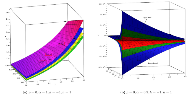
Fig. 2. Lower and upper bound surface solution with distinct values of α for Example 1. |
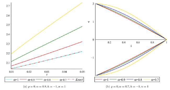
Fig. 3. Lower and upper bound surface solution with distinct values of α for Example 1. |

Fig. 4. Lower and upper bound solution profile with distinct values of α for Example 2. |
Example 2
Let us consider a nonlinear fifth-order FFKdVE:
$ \begin{aligned} \mathbf{D}_{\tau}^{\alpha} \tilde{\nu}(\varsigma, \tau)= & \tilde{\nu}(\varsigma, \tau) \otimes \frac{\partial^{3} \tilde{\nu}(\varsigma, \tau)}{\partial \varsigma^{3}} \ominus \frac{\partial^{5} \tilde{\nu}(\varsigma, \tau)}{\partial \varsigma^{5}} \\ & \ominus \tilde{\nu}(\varsigma, \tau) \otimes \frac{\partial \tilde{\nu}(\varsigma, \tau)}{\partial \varsigma} \end{aligned} $
with the fuzzy IC
$ \tilde{\nu}(\varsigma, 0)=\widetilde{B} \otimes e^{\varsigma} $
where $ \widetilde{B}=[-1,0,1] $ is an TFN. Also we can write in ℓ-cut, i.e., $ [\underline{B}, \bar{B}]=[\ell-1,1-\ell] $.
By means of Eqs. (8) to (14), Eqs. (48) and (49) can be rewritten in DP form as:
$ \begin{aligned} \mathbf{D}_{\tau}^{\alpha} \tilde{\nu}(\varsigma, \tau, \ell, \varrho)= & \tilde{\nu}(\varsigma, \tau, \ell, \varrho) \frac{\partial^{3} \tilde{\nu}(\varsigma, \tau, \ell, \varrho)}{\partial \varsigma^{3}}-\frac{\partial^{5} \tilde{\nu}(\varsigma, \tau, \ell, \varrho)}{\partial \varsigma^{5}} \\ & -\tilde{\nu}(\varsigma, \tau, \ell, \varrho) \frac{\partial \tilde{\nu}(\varsigma, \tau, \ell, \varrho)}{\partial \varsigma} \end{aligned} $
and
$ \widetilde{E}(\ell, \varrho)=\varrho\{\bar{B}-\underline{B}\}+\underline{B}=\varrho\{(2-\ell)\}+1-\ell \text {. } $
We can write the fuzzy IC in an DP form as
$ \tilde{\nu}(\varsigma, 0, \ell, \varrho)=\widetilde{E}(\ell, \varrho) e^{\varsigma} $
Upon considering the Shehu transform on Eq. (50) and using the IC on Eq. (51), we get
$ \begin{array}{l} \mathscr{P}[\tilde{\nu}(\varsigma, \tau, \ell, \varrho)] \\ -\frac{u}{s}\left(\widetilde{E}(\ell, \varrho) e^{\varsigma}\right)+\frac{u^{\alpha}}{s^{\alpha}} \mathscr{S}\left[\tilde{\nu}(\varsigma, \tau, \ell, \varrho) \frac{\partial^{3} \tilde{\nu}(\varsigma, \tau, \ell, \varrho)}{\partial \varsigma^{3}}\right. \\ \left.-\frac{\partial^{5} \tilde{\nu}(\varsigma, \tau, \ell, \varrho)}{\partial \varsigma^{5}}-\tilde{\nu}(\varsigma, \tau, \ell, \varrho) \frac{\partial \tilde{\nu}(\varsigma, \tau, \ell, \varrho)}{\partial \varsigma}\right] \end{array} $
The non-linear operator $\mathscr{N}$ can be rewritten via the proposed algorithm as follows:
$\begin{aligned} \mathscr{N} & {[\widetilde{w}(\varsigma, \tau, \ell, \varrho: q)] } \\ & =\mathscr{S}[\widetilde{w}(\varsigma, \tau, \ell, \varrho ; q)]-\frac{u}{s}\left(\frac{\widetilde{E}(\ell, \varrho)}{\varsigma}\right) \\ & +\frac{u^{\alpha}}{s^{\alpha}} \mathscr{S}\left[-\widetilde{w}(\varsigma, \tau, \ell, \varrho ; q) \frac{\partial^{3} \widetilde{w}(\varsigma, \tau, \ell, \varrho ; q)}{\partial \varsigma^{3}}\right. \\ & \left.+\frac{\partial^{5} \widetilde{w}(\varsigma, \tau, \ell, \varrho ; q)}{\partial \varsigma^{5}}+\widetilde{w}(\varsigma, \tau, \ell, \varrho ; q) \frac{\partial \widetilde{w}(\varsigma, \tau, \ell, \varrho ; q)}{\partial \varsigma}\right] \end{aligned}$
Application of the q-FHAShTM, the deformation equation of mth order at $\widetilde{H}(\varsigma, \tau)=1$ can be obtained as
$\mathbf{S}\left[\tilde{\nu}_{m}(\varsigma, \tau, \ell, \varrho)-\Psi_{m} \tilde{\nu}_{m-1}(\varsigma, \tau, \ell, \varrho)\right]=\hbar \Re_{m}\left(\overrightarrow{\vec{\nu}}_{m-1}(\varsigma, \tau, \ell, \varrho)\right)$
where
$\begin{array}{l} \Re_{\mathfrak{m}}\left(\overrightarrow{\tilde{\nu}}_{m-1}\right)=\mathbf{S}\left[\tilde{\nu}_{m-1}\right]-\left(1-\frac{\Psi_{m}}{n}\right) \frac{u}{s}\left(\widetilde{E}(\ell, \varrho) e^{\varsigma}\right) \\ +\frac{u^{\alpha}}{s^{\alpha}} \mathbf{S}\left[-\sum_{i=0}^{m-1} \tilde{\nu}_{i} \frac{\partial^{3} \tilde{\nu}_{m-1-i}}{\partial \varsigma^{3}}+\frac{\partial^{5} \tilde{\nu}_{m-1}(\varsigma, \tau, \ell, \varrho)}{\partial \varsigma^{5}}+\sum_{i=0}^{m-1} \tilde{\nu}_{i} \frac{\partial \tilde{\nu}_{m-1-i}}{\partial \varsigma}\right]. \end{array}$
Upon taking the inverse “Shehu transform” on both sides of Eq. (54), it obtain
$\begin{aligned} \tilde{\nu}_{m}(\varsigma, \tau, \ell, \varrho)= & \Psi_{m} \tilde{\nu}_{m-1}(\varsigma, \tau, \ell, \varrho) \\ & +\mathbf{S}^{-1}\left[\hbar \Re_{m}\left(\overrightarrow{\tilde{\nu}}_{m-1}\right)(\varsigma, \tau, \ell, \varrho)\right] \end{aligned}$
Thus, we get
$\tilde{\nu}_{0}(\varsigma, \tau, \ell, \varrho)=\widetilde{E}(\ell, \varrho) e^{\varsigma}$
$\tilde{\nu}_{1}(\varsigma, \tau, \ell, \varrho)=\frac{h \tilde{E}(\ell, \varrho) \tau^{\alpha} e^{\zeta}}{\Gamma(\alpha+1)}$
$\tilde{\nu}_{2}(\varsigma, \tau, \ell, \varrho)=\frac{h(h+n) \tilde{E}(\ell, \varrho) \tau^{\alpha} e^{\zeta}}{\Gamma(\alpha+1)}+\frac{h^{2} \tilde{E}(\ell, \varrho) \tau^{2 \alpha} e^{5}}{\Gamma(2 \alpha+1)}$
$\begin{aligned} \tilde{\nu}_{3}(\varsigma, \tau, \ell, \varrho)= & (h+n)\left\{\frac{h(h+n) \widetilde{E}(\ell, \varrho) \tau^{\alpha} e^{\varsigma}}{\Gamma(\alpha+1)}+\frac{h^{2} \widetilde{E}(\ell, \varrho) \tau^{2 \alpha} e^{\varsigma}}{\Gamma(2 \alpha+1)}\right\} \\ & +h\left\{\frac{h(h+n) \widetilde{E}(\ell, \varrho) \tau^{2 \alpha} e^{\varsigma}}{\Gamma(2 \alpha+1)}+\frac{h^{2} \widetilde{E}(\ell, \varrho) \tau^{3 \alpha} e^{\varsigma}}{\Gamma(3 \alpha+1)}\right\} \end{aligned}$
Thus the approximate analytical solution of Eq. (48) is
$\begin{aligned} \tilde{\nu}(\varsigma, \tau, \ell, \varrho)= & \tilde{\nu}_{0}(\varsigma, \tau, \ell, \varrho)+\frac{\tilde{\nu}_{1}(\varsigma, \tau, \ell, \varrho)}{n} \\ & +\frac{\left.\tilde{\nu}_{2} \varsigma, \tau, \ell, \varrho\right)}{n^{2}}+\frac{\tilde{\nu}_{3}(\varsigma, \tau, \ell, \varrho)}{n^{3}}+\ldots \end{aligned}$
Finally, we have
$\begin{aligned} \tilde{\nu} & (\varsigma, \tau, \ell, \varrho) \\ & =\widetilde{E}(\ell, \varrho) e^{\varsigma}+\frac{h \widetilde{E}(\ell, \varrho) \tau^{\alpha} e^{\varsigma}}{n \Gamma(\alpha+1)} \\ & +\frac{1}{n^{2}}\left\{\frac{h(h+n) \widetilde{E}(\ell, \varrho) \tau^{\alpha} e^{\varsigma}}{\Gamma(\alpha+1)}+\frac{h^{2} \widetilde{E}(\ell, \varrho) \tau^{2 \alpha} e^{\varsigma}}{\Gamma(2 \alpha+1)}\right\} \\ & +\frac{1}{n^{3}}\left\{(h+n)\left\{\frac{h(h+n) \widetilde{E}(\ell, \varrho) \tau^{\alpha} e^{\varsigma}}{\Gamma(\alpha+1)}+\frac{h^{2} \widetilde{E}(\ell, \varrho) \tau^{2 \alpha} e^{\varsigma}}{\Gamma(2 \alpha+1)}\right\}\right. \\ & \left.+h\left\{\frac{h(h+n) \widetilde{E}(\ell, \varrho) \tau^{2 \alpha} e^{\varsigma}}{\Gamma(2 \alpha+1)}+\frac{h^{2} \widetilde{E}(\ell, \varrho) \tau^{3 \alpha} e^{\varsigma}}{\Gamma(3 \alpha+1)}\right\}\right\}+\ldots \end{aligned}$
Now by using Definition 5 in Eq. (62), and letting ϱ=0, i.e., lower bound solution, we get
$\begin{array}{l} (\varsigma, \tau, \ell, \varrho)=\tilde{\nu}(\varsigma, \tau, 0)=[\tilde{\nu}(\varsigma, \tau)]^{\ell}=\underline{\nu}(\varsigma, \tau, \ell) \\ \underline{\nu}(\varsigma, \tau, \ell)=\underline{E}(\ell) e^{\varsigma} \\ \quad+\frac{h \underline{E}(\ell) \tau^{\alpha} e^{\varsigma}}{n \Gamma(\alpha+1)}+\frac{1}{n^{2}}\left\{\frac{h(h+n) \underline{E}(\ell) \tau^{\alpha} e^{\varsigma}}{\Gamma(\alpha+1)}+\frac{h^{2} \underline{E}(\ell) \tau^{2 \alpha} e^{\varsigma}}{\Gamma(2 \alpha+1)}\right\} \\ \quad+\frac{1}{n^{3}}\left\{(h+n)\left\{\frac{h(h+n) \underline{E}(\ell) \tau^{\alpha} e^{\varsigma}}{\Gamma(\alpha+1)}+\frac{h^{2} \underline{E}(\ell) \tau^{2 \alpha} e^{\varsigma}}{\Gamma(2 \alpha+1)}\right\}\right. \\ \left.\quad+h\left\{\frac{h(h+n) \underline{E}(\ell) \tau^{2 \alpha} e^{\varsigma}}{\Gamma(2 \alpha+1)}+\frac{h^{2} \underline{E}(\ell) \tau^{3 \alpha} e^{\varsigma}}{\Gamma(3 \alpha+1)}\right\}\right\}+\ldots \end{array}$
Thus by using Definition 5 in Eq. (62), and putting ϱ=1, i.e., lower bound solution and $\widetilde{E}(\ell, 0)=\underline{E}(\ell)$, we obtain
$\begin{array}{l} \tilde{\nu}(\varsigma, \tau, \ell, \varrho)=\tilde{\nu}(\varsigma, \tau, 1)=[\tilde{\nu}(\varsigma, \tau)]^{\ell}=\bar{\nu}(\varsigma, \tau, \ell) \\ \quad \bar{\nu}(\varsigma, \tau, \ell)=\bar{E}(\ell) e^{\varsigma} \\ \quad+\frac{h \bar{E}(\ell) \tau^{\alpha} e^{\varsigma}}{n \Gamma(\alpha+1)}+\frac{1}{n^{2}}\left\{\frac{h(h+n) \bar{E}(\ell) \tau^{\alpha} e^{\varsigma}}{\Gamma(\alpha+1)}+\frac{h^{2} \widetilde{E}(\ell) \tau^{2 \alpha} e^{\varsigma}}{\Gamma(2 \alpha+1)}\right\} \\ \quad+\frac{1}{n^{3}}\left\{(h+n)\left\{\frac{h(h+n) \bar{E}(\ell, \varrho) \tau^{\alpha} e^{\varsigma}}{\Gamma(\alpha+1)}+\frac{h^{2} \bar{E}(\ell) \tau^{2 \alpha} e^{\varsigma}}{\Gamma(2 \alpha+1)}\right\}\right. \\ \left.\quad+h\left\{\frac{h(h+n) \bar{E}(\ell) \tau^{2 \alpha} e^{\varsigma}}{\Gamma(2 \alpha+1)}+\frac{h^{2} \bar{E}(\ell) \tau^{3 \alpha} e^{\varsigma}}{\Gamma(3 \alpha+1)}\right\}\right\}+\ldots \end{array}$
Here, we report the obtained results in Tables 2, 3 and Fig. 5, Fig. 6, Fig. 7, Fig. 8, Fig. 9, Fig. 10 for various values α, ℓ and ϱ. Table 2 presents the comparison results of the exact solution with the approximate solution of the q-HAShTM in crisp case i.e for $\ell, \varrho \in\{0,1\}$. The graphical interpretation has been done for fractional-order α=1 and for fixed values ℓ=0 and ϱ=1 (crisp case) with varying ς and τ, where the values written for the HPTM solution were obtained using reference [46]. Table 3 compares the exact solution with the approximate solution of the q-HAShTM in uncertain case, i.e, ℓ and ϱ∈(0,1) for α=1 and for fixed values of the uncertain parameters, i.e., ℓ=0.2 and ϱ=0.1 with various values of ς and τ. The numerical results obtained for several grid points by the q-HAShTM are compared to the values of the exact solution with high precision up to the fourth term approximation. Fig. 5 depicts the approximate solution of the q-HAShTM under gH-differentiability of CFD of fractional order with α=1 and shows the exact solution of the problem in the crisp case, while the Fig. 6 shows this discussion in an uncertain case. Fig. 7 portraits the approximate solution of the q-HAShTM under gH-differentiability of CFD for different values of fractional order α∈{0.7,0.8,0.9,1} in crisp and uncertain case with varying values of ς and ϱ. It is worth noting that as the accuracies rise, so does the order of the approximation. Fig. 8 illustrates the two-dimensional approximate solutions of the q-HAShTM with different values of fractional order α∈{0.7,0.8,0.9,1} and for exact solution in crisp and in uncertain case, respectively. It can be noticed that as the as the accuracies rises, so does the order of approximation. Fig. 9 displays the lower and upper bound approximate solution of the q-HAShTM under gH-differentiability of CFD with different vales of fractional order α∈{0.7,0.8,0.9,1} and having fixed values ℓ=0.5, and ϱ=0.1,n=1, with varying values of ς and τ. Finally, Fig. 10 represents the h-curve for crisp and uncertain case and the solution is converges the value of h∈(−1.5,0) in crisp and uncertain case for different values of α.
Fig. 5. Approximate and exact solution profile in crisp case for Example 2. |
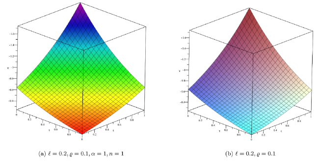
Fig. 6. Approximate and exact solution profile in uncertain case for Example 2. |
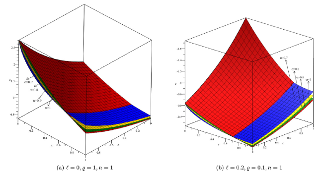
Fig. 7. Solution profile for distinct values of α in crisp and uncertain case for Example 2. |
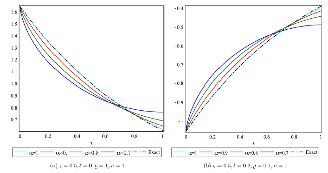
Fig. 8. Solution behaviour for distinct values of α in crisp and uncertain case for Example 2. |
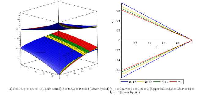
Fig. 9. Solution behaviour for distinct values of α in lower and upper bound for Example 2. |
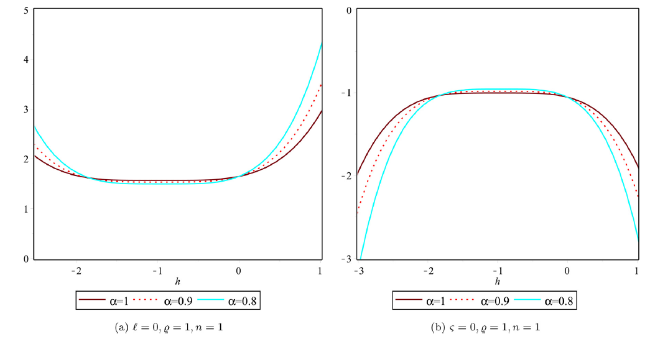
Fig. 10. Solution behaviour for distinct values of α in lower and upper bound for Example 2. |
Table 2. Comparision of exact and approximate solution of q-FHAShTM for distinct values of τ and ς and fixed parameters i.e. ℓ=0,ϱ=1 Example 2. |
| q-FHAShTM | ||||||||
|---|---|---|---|---|---|---|---|---|
| ς | τ | 1st-term | 2nd-term | 3rd-term | 4th-term | Exact | Error | Error |
| App. | App. | App. | App. | q-FHAShTM | HPTM [46] | |||
| 0.01 | 1.632234058 | 1.632316494 | 1.632316219 | 1.632316220 | 1.632316220 | 0.0 | 0.0 | |
| 0.02 | 1.615746846 | 1.616076590 | 1.616074392 | 1.616074403 | 1.616074402 | 1×10⁻⁹ | 1×10⁻⁹ | |
| 0.5 | 0.03 | 1.599259633 | 1.600001558 | 1.599994139 | 1.599994195 | 1.599994193 | 2×10⁻⁹ | 2×10⁻⁹ |
| 0.04 | 1.582772420 | 1.584091397 | 1.584073811 | 1.584073987 | 1.584073985 | 2×10⁻⁹ | 3×10⁻⁹ | |
| 0.05 | 1.566285207 | 1.568346109 | 1.568311761 | 1.568312190 | 1.568312185 | 5×10⁻⁹ | 2×10⁻⁹ | |
| 0.01 | 2.691234472 | 2.691234924 | 2.691234471 | 2.691234472 | 2.691234472 | 0.0 | 0.0 | |
| 0.02 | 2.664456242 | 2.664459847 | 2.664456223 | 2.664456241 | 2.664456242 | 1×10⁻⁹ | 2×10⁻⁹ | |
| 1.0 | 0.03 | 2.637944459 | 2.637956600 | 2.637944368 | 2.637944460 | 2.637944459 | 1×10⁻⁹ | 1×10⁻⁹ |
| 0.04 | 2.611696473 | 2.611725180 | 2.611696185 | 2.611696475 | 2.611696473 | 2×10⁻⁹ | 2×10⁻⁹ | |
| 0.05 | 2.585709659 | 2.585765589 | 2.585708958 | 2.585709666 | 2.585709659 | 7×10⁻⁹ | 6×10⁻⁹ |
Table 3. Comparision of exact and approximate solution of q-FHAShTM for distinct values of τ and ς and fixed parameters i.e ℓ=0.2,ϱ=0.1 (uncertain case, i.e, ℓ,ς≠0,1) of Example 2. |
| q-FHAShTM | |||||||
|---|---|---|---|---|---|---|---|
| τ | 1st-term | 2nd-term | 3rd-term | 4th-term | Exact | Error | |
| App. | App. | App. | App. | q-FHAShTM | |||
| 0.01 | -1.044629797 | -1.044682556 | -1.044682380 | -1.044682380 | -1.044682381 | 1×10⁻⁹ | |
| 0.02 | -1.034077981 | -1.034289017 | -1.034287610 | -1.034287617 | -1.034287617 | 0.0 | |
| 0.5 | 0.03 | -1.023526165 | -1.024000997 | -1.023996249 | -1.023996285 | -1.023996284 | 1×10⁻⁹ |
| 0.04 | -1.012974348 | -1.013818493 | -1.013807238 | -1.013807351 | -1.013807350 | 1×10⁻⁹ | |
| 0.05 | -1.002422532 | -1.003741509 | -1.003719526 | -1.003719801 | -1.003719798 | 3×10⁻⁹ | |
| 0.01 | -1.722303366 | -1.722390351 | -1.722390061 | -1.722390062 | -1.722390062 | 0.0 | |
| 0.02 | -1.704906363 | -1.705254303 | -1.705251983 | -1.705251995 | -1.705251995 | 0.0 | |
| 1.0 | 0.03 | -1.687509359 | -1.688292224 | -1.688284395 | -1.688284454 | -1.688284454 | 0.0 |
| 0.04 | -1.670112355 | -1.671504115 | -1.671485558 | -1.671485744 | -1.671485743 | 1×10⁻⁹ | |
| 0.05 | -1.652715352 | -1.654889977 | -1.654853733 | -1.654854186 | -1.654854182 | 4×10⁻⁹ |
Example 3
Consider the nonlinear FFKdVE as:
$\mathbf{D}_{T}^{\alpha} \tilde{\nu}(\varsigma, \tau)=\ominus \frac{\partial^{3} \tilde{\nu}(\varsigma, \tau)}{\partial \varsigma^{s}} \ominus 2 \otimes \frac{\partial \hat{\nu}(\varsigma, \tau)}{\partial \varsigma},$
with the fuzzy IC
$\tilde{\nu}(\varsigma, 0)=\widetilde{B} \otimes \sin (\varsigma)$
where $\widetilde{B}=[-1,0,1]$ is an TFN. Also we can write it in ℓ-cut i.e.$ [\underline{B}, \bar{B}]=[\ell-1,1-\ell]$
Based on Eqs. (8) to (14), Eqs. (65) to (66) can be restated in DP form as:
$ \mathbf{D}_{T}^{\alpha} \tilde{\nu}(\varsigma, \tau, \ell, \varrho)=-\frac{\partial^{8} \tilde{\nu}(\varsigma, \tau, \ell, \varrho}{\partial \varsigma^{3}}-2 \frac{\partial \tilde{\nu}(\varsigma, \tau, \ell, \varrho)}{\partial \varsigma} $
and
$ \widetilde{E}(\ell, \varrho)=\varrho\{\bar{B}-\underline{B}\}+\underline{B}=\varrho\{(2-\ell)\}+1-\ell. $
We can write fuzzy IC’s in an DP form as
$ \tilde{\nu}(\varsigma, 0, \ell, \varrho)=\widetilde{E}(\ell, \varrho) \sin (\varsigma) $
Upon employing the Shehu transform on Eq. (67) and using the IC on Eq. (68), we get
$ \begin{aligned} \mathscr{S}[\tilde{\nu}(\varsigma, \tau, \ell, \varrho)]- & \frac{u}{s}(\widetilde{E}(\ell, \varrho) \sin (\varsigma)) \\ & +\frac{u^{\alpha}}{s^{\alpha}} \mathscr{S}\left[-\frac{\partial^{3} \tilde{\nu}(\varsigma, \tau, \ell, \varrho)}{\partial \varsigma^{3}}-2 \frac{\partial \tilde{\nu}(\varsigma, \tau, \ell, \varrho)}{\partial \varsigma}\right]. \end{aligned} $
The non-linear operator $ \mathscr{N} $ can be represented by using the proposed algorithm as follows:
$ \begin{array}{l} \mathscr{N}[\widetilde{w}(\varsigma, \tau, \ell, \varrho: q)]=\mathscr{S}[\widetilde{w}(\varsigma, \tau, \ell, \varrho ; q)]-\left(\frac{u}{s}\right)(\widetilde{E}(\ell, \varrho) \sin (\varsigma)) \\ \quad+\frac{u^{\alpha}}{s^{\alpha}} \mathscr{S}\left[\frac{\partial^{3} \widetilde{w}(\varsigma, \tau, \ell, \varrho ; q)}{\partial \varsigma^{3}}+2 \frac{\partial \widetilde{w}(\varsigma, \tau, \ell, \varrho ; q)}{\partial \varsigma}\right]. \end{array} $
Using the q-FHAShTM, the deformation equation of m-th order at $ \widetilde{H}(\varsigma, \tau)=1 $ can be obtained as:
$ \mathbf{S}\left[\tilde{\nu}_{m}(\varsigma, \tau, \ell, \varrho)-\Psi_{m} \tilde{\nu}_{m-1}(\varsigma, \tau, \ell, \varrho)\right]=\hbar \Re_{m}\left(\overrightarrow{\vec{\nu}}_{m-1}(\varsigma, \tau, \ell, \varrho)\right) $
where
$ \begin{aligned} \Re_{\mathfrak{m}}\left(\overrightarrow{\vec{\nu}}_{m-1}\right)= & \mathbf{S}\left[\tilde{\nu}_{m-1}\right]-\left(1-\frac{\Psi_{m}}{n}\right)\left(\frac{u}{s}\right)(\widetilde{E}(\ell, \varrho) \sin (\varsigma)) \\ & +\frac{u^{\alpha}}{s^{\alpha}} \mathbf{S}\left[\frac{\partial^{3} \tilde{\nu}_{m-1}}{\partial \varsigma^{3}}+2 \frac{\partial \tilde{\nu}_{m-1}}{\partial \varsigma}\right]. \end{aligned} $
By means of the inverse “Shehu transform” to both sides of Eq. (71), we get
$ \begin{aligned} \tilde{\nu}_{m}(\varsigma, \tau, \ell, \varrho)= & \Psi_{m} \tilde{\nu}_{m-1}(\varsigma, \tau, \ell, \varrho) \\ & +\mathbf{S}^{-1}\left[\hbar \Re_{m}\left(\overrightarrow{\tilde{\nu}}_{m-1}\right)(\varsigma, \tau, \ell, \varrho)\right] \end{aligned} $
Solving the aforementioned equation systematically, we obtain
$ \tilde{\nu}_{0}(\varsigma, \tau, \ell, \varrho)=\widetilde{E}(\ell, \varrho) \sin (\varsigma) $
$ \tilde{\nu}_{1}(\varsigma, \tau, \ell, \varrho)=\frac{h \tilde{E}(\ell, e) \tau^{\alpha} \cos (\varsigma)}{\Gamma(\alpha+1)} $
$ \tilde{\nu}_{2}(\varsigma, \tau, \ell, \varrho)=\frac{h(h+n) \tilde{E}(\ell, \varrho) \tau^{\alpha} \cos (\varsigma)}{\Gamma(\alpha+1)}-\frac{h^{2} \tilde{E}(\ell, \varrho) \tau^{2 a} \sin (\varsigma)}{\Gamma(2 \alpha+1)} $
$ \begin{array}{l} \tilde{\nu}_{3}(\varsigma, \tau, \ell, \varrho) \\ \quad=(h+n)\left\{\frac{h(h+n) \widetilde{E}(\ell, \varrho) \tau^{\alpha} \cos (\varsigma)}{\Gamma(\alpha+1)}-\frac{h^{2} \widetilde{E}(\ell, \varrho) \tau^{2 \alpha} \sin (\varsigma)}{\Gamma(2 \alpha+1)}\right\} \\ \quad+h\left\{-\frac{h(h+n) \widetilde{E}(\ell, \varrho) \tau^{2 \alpha} \sin (\varsigma)}{\Gamma(2 \alpha+1)}-\frac{h^{2} \widetilde{E}(\ell, \varrho) \tau^{3 \alpha} \cos (\varsigma)}{\Gamma(3 \alpha+1)}\right\} \end{array} $
$ \begin{array}{l} \begin{array}{l} \tilde{\nu}_{4}(\varsigma, \tau, \ell, \varrho) \\ =(h+n)^{2}\left\{\frac{h(h+n) \widetilde{E}(\ell, \varrho) \tau^{\alpha} \cos (\varsigma)}{\Gamma(\alpha+1)}-\frac{h^{2} \widetilde{E}(\ell, \varrho) \tau^{2 \alpha} \sin (\varsigma)}{\Gamma(2 \alpha+1)}\right\}+ \\ -h^{2}\left\{\frac{h(h+n) \widetilde{E}(\ell, \varrho) \tau^{3 \alpha} \cos (\varsigma)}{\Gamma(3 \alpha+1)}-\frac{h^{2} \widetilde{E}(\ell, \varrho) \tau^{4 \alpha} \sin (\varsigma)}{\Gamma(4 \alpha+1)}\right\} \\ +2 h(h+n)\left\{-\frac{h(h+n) \widetilde{E}(\ell, \varrho) \tau^{2 \alpha} \sin (\varsigma)}{\Gamma(2 \alpha+1)}\right. \\ \left.-\frac{h^{2} \widetilde{E}(\ell, \varrho) \tau^{3 \alpha} \cos (\varsigma)}{\Gamma(3 \alpha+1)}\right\}+ \end{array}\\ \tilde{\nu}_{4}(\varsigma, \tau, \ell, \varrho)\\ =(h+n)^{2}\left\{\frac{h(h+n) \widetilde{E}(\ell, \varrho) \tau^{\alpha} \cos (\varsigma)}{\Gamma(\alpha+1)}-\frac{h^{2} \widetilde{E}(\ell, \varrho) \tau^{2 \alpha} \sin (\varsigma)}{\Gamma(2 \alpha+1)}\right\}+\\ -h^{2}\left\{\frac{h(h+n) \widetilde{E}(\ell, \varrho) \tau^{3 \alpha} \cos (\varsigma)}{\Gamma(3 \alpha+1)}-\frac{h^{2} \widetilde{E}(\ell, \varrho) \tau^{4 \alpha} \sin (\varsigma)}{\Gamma(4 \alpha+1)}\right\}\\ +2 h(h+n)\left\{-\frac{h(h+n) \widetilde{E}(\ell, \varrho) \tau^{2 \alpha} \sin (\varsigma)}{\Gamma(2 \alpha+1)}\right.\\ \left.-\frac{h^{2} \widetilde{E}(\ell, \varrho) \tau^{3 \alpha} \cos (\varsigma)}{\Gamma(3 \alpha+1)}\right\}+ \end{array} $
Therefore, the approximate analytical solution of Eq. (65) can be obtained as
$ \begin{aligned} \tilde{\nu}(\varsigma, \tau, \ell, \varrho)= & \tilde{\nu}_{0}(\varsigma, \tau, \ell, \varrho)+\frac{\tilde{\nu}_{1}(\varsigma, \tau, \ell, \varrho)}{n} \\ & +\frac{\left.\tilde{\nu}_{2} \varsigma, \tau, \ell, \varrho\right)}{n^{2}}+\frac{\tilde{\nu}_{3}(\varsigma, \tau, \ell, \varrho)}{n^{3}}+\ldots \end{aligned} $
Finally, we have
$ \begin{array}{l} \tilde{\nu}(\varsigma, \tau, \ell, \varrho)=\widetilde{E}(\ell, \varrho) \sin (\varsigma)+\frac{h \widetilde{E}(\ell, \varrho) \tau^{\alpha} \cos (\varsigma)}{n \Gamma(\alpha+1)} \\ +\frac{1}{n^{2}}\left\{\frac{h(h+n) \widetilde{E}(\ell, \varrho) \tau^{\alpha} \cos (\varsigma)}{\Gamma(\alpha+1)}-\frac{h^{2} \widetilde{E}(\ell, \varrho) \tau^{2 \alpha} \sin (\varsigma)}{\Gamma(2 \alpha+1)}\right\} \\ +\frac{1}{n^{3}}\left\{( h + n ) \left\{\frac{h(h+n) \widetilde{E}(\ell, \varrho) \tau^{\alpha} \cos (\varsigma)}{\Gamma(\alpha+1)}\right.\right. \\ \left.-\frac{h^{2} \widetilde{E}(\ell, \varrho) \tau^{2 \alpha} \sin (\varsigma)}{\Gamma(2 \alpha+1)}\right\} \\ \left(+h\left\{-\frac{h(h+n) \widetilde{E}(\ell, \varrho) \tau^{2 \alpha} \sin (\varsigma)}{\Gamma(2 \alpha+1)}-\frac{h^{2} \widetilde{E}(\ell, \varrho) \tau^{3 \alpha} \cos (\varsigma)}{\Gamma(3 \alpha+1)}\right\}\right\}+\ldots \end{array} $
Referring Definition 5 in Eq. (80) and putting $ \varrho=0 $, i.e., lower bound solution, we obtain
$ \begin{array}{l} \tilde{\nu}(\varsigma, \tau, \ell, \varrho)=\tilde{\nu}(\varsigma, \tau, 0)=[\tilde{\nu}(\varsigma, \tau)]^{\ell}=\underline{\nu}(\varsigma, \tau, \ell) \\ \underline{\nu}(\varsigma, \tau, \ell)=\underline{E}(\ell) \sin (\varsigma)+\frac{h \underline{E}(\ell) \tau^{\alpha} \cos (\varsigma)}{n \Gamma(\alpha+1)} \\ +\frac{1}{n^{2}}\left\{\frac{h(h+n) \widetilde{E}(\ell) \tau^{\alpha} \cos (\varsigma)}{\Gamma(\alpha+1)}-\frac{h^{2} \underline{E}(\ell) \tau^{2 \alpha} \sin (\varsigma)}{\Gamma(2 \alpha+1)}\right\} \\ +\frac{1}{n^{3}}\left\{(h+n)\left\{\frac{h(h+n) \underline{E}(\ell) \tau^{\alpha} \cos (\varsigma)}{\Gamma(\alpha+1)}-\frac{h^{2} \widetilde{E}(\ell) \tau^{2 \alpha} \sin (\varsigma)}{\Gamma(2 \alpha+1)}\right\}\right. \\ \left.+h\left\{-\frac{h(h+n) \underline{E}(\ell) \tau^{2 \alpha} \sin (\varsigma)}{\Gamma(2 \alpha+1)}-\frac{h^{2} \underline{E}(\ell) \tau^{3 \alpha} \cos (\varsigma)}{\Gamma(3 \alpha+1)}\right\}\right\}+\ldots \end{array} $
By using Definition 5 in Eq. (81), and putting $ \varrho=1 $, i.e., lower bound solution and $\widetilde{E}(\ell, 0)=\underline{E}(\ell)$, we have
$\begin{array}{l} \tilde{\nu}(\varsigma, \tau, \ell, \varrho)=\tilde{\nu}(\varsigma, \tau, 1)=[\tilde{\nu}(\varsigma, \tau)]^{\ell}=\bar{\nu}(\varsigma, \tau, \ell) \\ \\ \bar{\nu}(\varsigma, \tau, \ell)=\bar{E}(\ell) \sin (\varsigma)+\frac{h \bar{E}(\ell) \tau^{\alpha} \cos (\varsigma)}{n \Gamma(\alpha+1)} \\ \quad+\frac{1}{n^{2}}\left\{\frac{h(h+n) \bar{E}(\ell) \tau^{\alpha} \cos (\varsigma)}{\Gamma(\alpha+1)}-\frac{h^{2} \bar{E}(\ell) \tau^{2 \alpha} \sin (\varsigma)}{\Gamma(2 \alpha+1)}\right\} \\ \quad+\frac{1}{n^{3}}\left\{(h+n)\left\{\frac{h(h+n) \bar{E}(\ell) \tau^{\alpha} \cos (\varsigma)}{\Gamma(\alpha+1)}-\frac{h^{2} \bar{E}(\ell) \tau^{2 \alpha} \sin (\varsigma)}{\Gamma(2 \alpha+1)}\right\}\right. \\ \left.\quad+h\left\{-\frac{h(h+n) \bar{E}(\ell) \tau^{2 \alpha} \sin (\varsigma)}{\Gamma(2 \alpha+1)}-\frac{h^{2} \bar{E}(\ell) \tau^{3 \alpha} \cos (\varsigma)}{\Gamma(3 \alpha+1)}\right\}\right\}+\ldots \end{array}$
In what follows, we report the obtained results in Tables 4, 5 and Fig. 11, Fig. 12, Fig. 13, Fig. 14, Fig. 15, Fig. 16 for several values α, ℓ and ϱ. Table 4 compares the results of the exact and the approximate solution of the q-HAShTM in crisp case, i.e., ℓ and $\varrho \in\{0,1\}$. The fractional-order is assumed to α=1 with fixed values ℓ=0 and ϱ=1 in crisp case with varying values of ς and τ, where the values written for the HPTM solution were obtained using reference [41]. Table 5 represents the numerical comparison of exact and the approximate solution of the q-HAShTM in an uncertain case, i.e, when ℓ and ϱ∈(0,1) and α=1 for fixed values of uncertain parameters ℓ=0.2 and,ϱ=0.1 with various values of ς and τ. The numerical results of the problem at several grid points are obtained by the q-HAShTM and are compared with the numerical values of the exact solution with high precision up to fourth term approximation. Fig. 11 represents the approximate solution of the q-HAShTM under gH-differentiability of CFD with fractional order α=1 and shows the exact solution in the crisp case, while Fig. 12 illustrates the analysis in the uncertain case. Fig. 13 depicts the approximate solution of the q-HAShTM under gH-differentiability of CFD with different values of fractional order α∈{0.7,0.8,0.9,1} in crisp and in uncertain case with varying values of ς and ϱ. It is worth noting that as the accuracies of the solution be rises, so does the order of the approximation. Fig. 14 draws the two-dimensional approximate solutions of the q-HAShTM with different values of fractional order α∈{0.7,0.8,0.9,1} and the exact solution in the crisp case and in an uncertain case. Here, it can also be noticed that as the accuracies rise, the order of approximation becomes stable. Fig. 15 shows the lower and upper bound approximate solution of the q-HAShTM under gH-differentiability of CFD with different fractional order values α∈{0.7,0.8,0.9,1} and for fixed values ℓ=0.5,ϱ=0,1,n=1, with varying values ς and τ. Finally, Fig. 16 displays the h-curve for crisp and uncertain case and the solution is converges the value of h∈(−1.7,0) and h∈(−2,0) in crisp and uncertain case for different values of α.
Table 4. Comparision of exact and approximate solution of q-FHAShTM for different values of τ and ς and fixed parameters, i.e., ℓ=0,ϱ=1 of Example 3. |
| q-FHAShTM | ||||||||
|---|---|---|---|---|---|---|---|---|
| ς | τ | 1st-term | 2nd-term | 3rd-term | 4th-term | Exact | Error | Error |
| App. | App. | App. | App. | q-FHAShTM | LADM [41] | |||
| 0.01 | 0.4706497130 | 0.4706257417 | 0.4706258880 | 0.4706258882 | 0.4706258882 | 0.0 | 1.0×10⁻¹⁰ | |
| 0.02 | 0.4618738874 | 0.4617780023 | 0.4617791724 | 0.4617791756 | 0.4617791755 | 1.0×10⁻¹⁰ | 1.0×10⁻⁹ | |
| 0.5 | 0.03 | 0.4530980617 | 0.4528823202 | 0.4528862693 | 0.4528862855 | 0.4528862854 | 1.0×10⁻¹⁰ | 1.0×10⁻⁹ |
| 0.04 | 0.4443222361 | 0.4439386957 | 0.4439480566 | 0.4439481077 | 0.4439481070 | 7.0×10⁻¹⁰ | 4.0×10⁻⁹ | |
| 0.05 | 0.4355464105 | 0.4349471286 | 0.4349654116 | 0.4349655365 | 0.4349655341 | 2.4×10⁻⁹ | 3.2×10⁻⁹ | |
| 0.01 | 0.8360679617 | 0.8360258882 | 0.8360259783 | 0.8360259787 | 0.8360259786 | 1.0×10⁻¹⁰ | 2.0×10⁻⁹ | |
| 0.02 | 0.8306649387 | 0.8304966445 | 0.8304973649 | 0.8304973705 | 0.8304973705 | 0.0 | 1.0×10⁻¹⁰ | |
| 1.0 | 0.03 | 0.8252619156 | 0.8248832537 | 0.8248856851 | 0.8248857135 | 0.8248857133 | 2.0×10⁻¹⁰ | 1.0×10⁻⁹ |
| 0.04 | 0.8198588926 | 0.8191857158 | 0.8191914790 | 0.8191915688 | 0.8191915683 | 5.0×10⁻¹⁰ | 1.0×10⁻⁹ | |
| 0.05 | 0.8144558695 | 0.8134040308 | 0.8134152871 | 0.8134155062 | 0.8134155048 | 1.4×10⁻⁹ | 1.2×10⁻⁹ |
Table 5. Comparision of exact and approximate solution of q-FHAShTM for distinct values of τ and ς and fixed parameters i.e. ℓ=0.2,ϱ=0.1 (uncetain case, i.e, ℓ,ς≠0,1) of Example 3. |
| q-FHAShTM | |||||||
|---|---|---|---|---|---|---|---|
| ς | τ | 1st-term | 2nd-term | 3rd-term | 4th-term | Exact | Error |
| App. | App. | App. | App. | q-FHAShTM | |||
| 0.01 | -0.3012158163 | -0.3012004747 | -0.3012005683 | -0.3012005684 | -0.301200568 | 0.0 | |
| 0.02 | -0.2955992879 | -0.2955379214 | -0.2955386703 | -0.2955386723 | -0.295538672 | 0.0 | |
| 0.5 | 0.03 | -0.2899827595 | -0.2898446849 | -0.2898472123 | -0.2898472227 | -0.289847222 | 0.0 |
| 0.04 | -0.2843662311 | -0.2841207652 | -0.2841267562 | -0.2841267889 | -0.284126788 | 4.0×10⁻¹⁰ | |
| 0.05 | -0.2787497027 | -0.2783661623 | -0.2783778634 | -0.2783779433 | -0.278377941 | 1.5×10⁻⁹ | |
| 0.01 | -0.5350834955 | -0.5350565684 | -0.5350566260 | -0.5350566262 | -0.535056626 | 1.0×10⁻¹⁰ | |
| 0.02 | -0.5316255608 | -0.5315178525 | -0.5315183136 | -0.5315183172 | -0.531518317 | 1.0×10⁻¹⁰ | |
| 1.0 | 0.03 | -0.5281676260 | -0.5279252824 | -0.5279268385 | -0.5279268567 | -0.527926856 | 2.0×10⁻¹⁰ |
| 0.04 | -0.5247096913 | - 0.5242788582 | -0.5242825467 | -0.5242826041 | -0.524282603 | 4.0×10⁻¹⁰ | |
| 0.05 | -0.5212517565 | -0.5205785797 | -0.5205857837 | - 0.5205859239 | -0.520585923 | 8.0×10⁻¹⁰ |
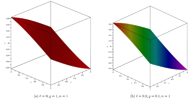
Fig. 11. Approximate and exact solution profile in crisp case for Example 3. |
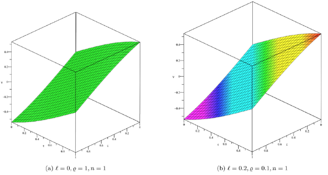
Fig. 12. Approximate and exact solution profile in uncertain case for Example 3. |
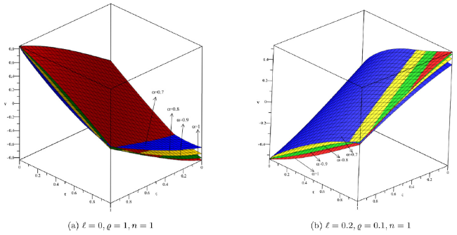
Fig. 13. Solution profile of distinct values of α in crisp and uncertain case for Example 3. |
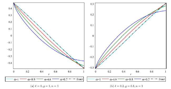
Fig. 14. Solution behavior for distinct values of α in crisp and uncertain case for Example 3. |
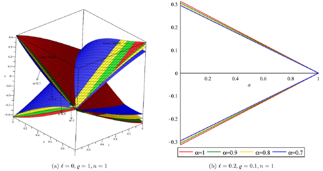
Fig. 15. Solution behaviour of distinct values of α in lower and upper bound for Example 3. |
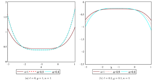
Fig. 16. Solution behaviour for distinct values of α in lower and upper bound for Example 3. |
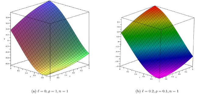
Fig. 17. Solution profile of distinct values of α in crisp case for Example 4. |
Example 4
We consider the FFKdVE as follows:
$\mathbf{D}_{\tau}^{\alpha} \tilde{\nu}(\varsigma, \tau)=\ominus \frac{\partial^{3} \tilde{\nu}\left(\varsigma_{1}, \varsigma_{2}, \tau\right)}{\partial_{\varsigma_{1}^{3}}^{3}} \ominus \frac{\partial^{3} \tilde{\nu}\left(\varsigma_{1}, \varsigma_{2}, \tau\right)}{\partial \varsigma_{2}^{3}}$
with fuzzy IC
$\tilde{\nu}\left(\varsigma_{1}, \varsigma_{2}, 0\right)=\widetilde{B} \otimes \cos \left(\varsigma_{1}+\varsigma_{2}\right),$
where $\widetilde{B}=[-1,0,1]$ is an TFN. Also we can write in ℓ-cut, that is, $[\underline{B}, \bar{B}]=[\ell-1,1-\ell]$.
With the help of Eqs. (8) to (14), Eqs. (83) and (84) can be rewritten in double parametric form as
$\mathbf{D}_{\tau}^{\alpha} \tilde{\nu}\left(\varsigma_{1}, \varsigma_{2}, \tau, \ell, \varrho\right)=-\frac{\partial^{3} \tilde{\nu}\left(\varsigma_{1}, \varsigma_{2}, \tau, \ell, \varrho\right.}{\partial \varsigma_{1}^{3}}-\frac{\partial^{3} \tilde{\nu}\left(\varsigma_{1}, \varsigma_{2}, \tau, \ell, \varrho\right)}{\partial \varsigma_{2}^{s}}$
and
$\widetilde{E}(\ell, \varrho)=\varrho\{\bar{B}-\underline{B}\}+\underline{B}=\varrho\{(2-\ell)\}+1-\ell.$
We can write fuzzy IC in a double parametric form
$\tilde{\nu}\left(\varsigma_{1}, \varsigma_{2}, 0, \ell, \varrho\right)=\widetilde{E}(\ell, \varrho) \cos \left(\varsigma_{1}+\varsigma_{2}\right)$
Upon applying the Shehu transform on Eq. (85) and using the IC on Eq. (86), we get
$\begin{array}{l} \mathscr{S}\left[\tilde{\nu}\left(\varsigma_{1}, \varsigma_{2}, \tau, \ell, \varrho\right)\right]-\frac{u}{s}\left(\widetilde{E}(\ell, \varrho) \cos \left(\varsigma_{1}+\varsigma_{2}\right)\right) \\ \quad+\frac{u^{\alpha}}{s^{\alpha}} \mathscr{S}\left[-\frac{\partial^{3} \tilde{\nu}\left(\varsigma_{1}, \varsigma_{2}, \tau, \ell, \varrho\right)}{\partial \varsigma_{1}^{3}}-\frac{\partial^{3} \tilde{\nu}\left(\varsigma_{1}, \varsigma_{2}, \tau, \ell, \varrho\right)}{\partial \varsigma_{2}^{3}}\right]. \end{array}$
The non-linear operator $\mathscr{N}$ can be defined based on the proposed algorithm as follows:
$\begin{array}{l} \mathscr{N}\left[\widetilde{w}\left(\varsigma_{1}, \varsigma_{2}, \tau, \ell, \varrho: q\right)\right]=\mathscr{S}\left[\widetilde{w}\left(\varsigma_{1}, \varsigma_{2}, \tau, \ell, \varrho ; q\right)\right] \\ \quad-\left(\frac{u}{s}\right)\left(\widetilde{E}(\ell, \varrho) \cos \left(\varsigma_{1}+\varsigma_{2}\right)\right) \\ \quad+\frac{u^{\alpha}}{s^{\alpha}} \mathscr{S}\left[\frac{\partial^{3} \widetilde{w}\left(\varsigma_{1}, \varsigma_{2}, \tau, \ell, \varrho ; q\right)}{\partial \varsigma_{1}^{3}}+\frac{\partial^{3} \widetilde{w}\left(\varsigma_{1}, \varsigma_{2}, \tau, \ell, \varrho ; q\right)}{\partial \varsigma_{2}^{3}}\right] \end{array}$
Now by using the q-FHAShTM, the deformation equation of m-th order at $\widetilde{H}\left(\varsigma_{1}, \varsigma_{2}, \tau\right)=1$ can be obtained as
$\begin{aligned} \mathbf{S}\left[\tilde{\nu}_{m}\left(\varsigma_{1}, \varsigma_{2}, \tau, \ell, \varrho\right)-\right. & \left.\Psi_{m} \tilde{\nu}_{m-1}\left(\varsigma_{1}, \varsigma_{2}, \tau, \ell, \varrho\right)\right] \\ & =\hbar \Re_{m}\left(\overrightarrow{\tilde{\nu}}_{m-1}\left(\varsigma_{1}, \varsigma_{2}, \tau, \ell, \varrho\right)\right) \end{aligned}$
where
$\begin{aligned} \Re_{\mathfrak{m}}\left(\overrightarrow{\tilde{\nu}}_{m-1}\right)= & \mathbf{S}\left[\tilde{\nu}_{m-1}\right]-\left(1-\frac{\Psi_{m}}{n}\right)\left(\frac{u}{s}\right)\left(\widetilde{E}(\ell, \varrho) \cos \left(\varsigma_{1}+\varsigma_{2}\right)\right) \\ & +\frac{u^{\alpha}}{s^{\alpha}} \mathbf{S}\left[\frac{\partial^{3} \tilde{\nu}_{m-1}}{\partial \varsigma_{1}^{3}}+\frac{\partial \tilde{\nu}_{m-1}}{\partial \varsigma_{2}^{3}}\right] \end{aligned}$
Upon applying the inverse Shehu transform to both sides of Eq. (89), we get
$\begin{aligned} \tilde{\nu}_{m}\left(\varsigma_{1}, \varsigma_{2}, \tau, \ell, \varrho\right)= & \Psi_{m} \tilde{\nu}_{m-1}\left(\varsigma_{1}, \varsigma_{2}, \tau, \ell, \varrho\right) \\ & +\mathbf{S}^{-1}\left[\hbar R_{\mathrm{m}}\left(\overrightarrow{\tilde{\nu}}_{m-1}\right)\left(\varsigma_{1}, \varsigma_{2}, \tau, \ell, \varrho\right)\right] \end{aligned}$
We arrive at by systematically solving the above equation,
$\tilde{\nu}_{0}\left(\varsigma_{1}, \varsigma_{2}, \tau, \ell, \varrho\right)=\widetilde{E}(\ell, \varrho) \cos \left(\varsigma_{1}+\varsigma_{2}\right)$
$\tilde{\nu}_{1}\left(\varsigma_{1}, \varsigma_{2}, \tau, \ell, \varrho\right)=\frac{2 h \tilde{E}(\ell, e) \tau^{\alpha} \sin \left(\varsigma_{1}+\varsigma_{2}\right)}{\Gamma(\alpha+1)}$
$\begin{aligned} \tilde{\nu}_{2}\left(\varsigma_{1}, \varsigma_{2}, \tau, \ell, \varrho\right)= & \frac{2 h(h+n) \widetilde{E}(\ell, \varrho) \tau^{\alpha} \sin \left(\varsigma_{1}+\varsigma_{2}\right)}{\Gamma(\alpha+1)} \\ & -\frac{4 h^{2} \widetilde{E}(\ell, \varrho) \tau^{2 \alpha} \cos \left(\varsigma_{1}+\varsigma_{2}\right)}{\Gamma(2 \alpha+1)} \end{aligned}$
$\begin{array}{l} \tilde{\nu}_{3}(\varsigma, \tau, \ell, \varrho) \\ =(h+n)\left\{\frac{2 h(h+n) \widetilde{E}(\ell, \varrho) \tau^{\alpha} \sin \left(\varsigma_{1}+\varsigma_{2}\right)}{\Gamma(\alpha+1)}\right. \\ \left.-\frac{4 h^{2} \widetilde{E}(\ell, \varrho) \tau^{2 \alpha} \cos \left(\varsigma_{1}+\varsigma_{2}\right)}{\Gamma(2 \alpha+1)}\right\} \\ + h\left\{-\frac{4 h(h+n) \widetilde{E}(\ell, \varrho) \tau^{2 \alpha} \cos \left(\varsigma_{1}+\varsigma_{2}\right)}{\Gamma(2 \alpha+1)}\right. \\ \left.-\frac{8 h^{2} \widetilde{E}(\ell, \varrho) \tau^{3 \alpha} \sin \left(\varsigma_{1}+\varsigma_{2}\right)}{\Gamma(3 \alpha+1)}\right\} \end{array}$
$\begin{array}{l} \begin{array}{l} \tilde{\nu}_{4}\left(\varsigma_{1}, \varsigma_{2}, \tau, \ell, \varrho\right) \\ =(h+n)^{2}\left\{\frac{2 h(h+n) \tilde{E}(\ell, \varrho) \tau^{\alpha} \sin \left(\varsigma_{1}+\varsigma_{2}\right)}{\Gamma(\alpha+1)}\right. \\ \left.-\frac{4 h^{2} \widetilde{E}(\ell, \varrho) \tau^{2 \alpha} \cos \left(\varsigma_{1}+\varsigma_{2}\right)}{\Gamma(2 \alpha+1)}\right\} \\ +h(h+n)\left\{\frac{-4 h(h+n) \widetilde{E}(\ell, \varrho) \tau^{2 \alpha} \cos \left(\varsigma_{1}+\varsigma_{2}\right)}{\Gamma(2 \alpha+1)}\right. \\ \left.-\frac{8 h^{2} \widetilde{E}(\ell, \varrho) \tau^{3 \alpha} \sin \left(\varsigma_{1}+\varsigma_{2}\right)}{\Gamma(3 \alpha+1)}\right\} \\ +2 h(h+n)\left\{-\frac{2 h(h+n) \tilde{E}(\ell, \varrho) \tau^{2 \alpha} \cos \left(\varsigma_{1}+\varsigma_{2}\right)}{\Gamma(2 \alpha+1)}\right. \\ \left.-\frac{4 h^{2} \widetilde{E}(\ell, \varrho) \tau^{3 \alpha} \sin \left(\varsigma_{1}+\varsigma_{2}\right)}{\Gamma(3 \alpha+1)}\right\} \\ +2 h^{2}\left\{-\frac{4 h(h+n) \widetilde{E}(\ell, \varrho) \tau^{3 \alpha} \sin \left(\varsigma_{1}+\varsigma_{2}\right)}{\Gamma(3 \alpha+1)}\right. \\ \left.+\frac{8 h^{2} \tilde{E}(\ell, \varrho) \tau^{4 \alpha} \cos \left(\varsigma_{1}+\varsigma_{2}\right)}{\Gamma(4 \alpha+1)}\right\}. \end{array}\\ \tilde{\nu}_{4}\left(\varsigma_{1}, \varsigma_{2}, \tau, \ell, \varrho\right)\\ =(h+n)^{2}\left\{\frac{2 h(h+n) \tilde{E}(\ell, \varrho) \tau^{\alpha} \sin \left(\varsigma_{1}+\varsigma_{2}\right)}{\Gamma(\alpha+1)}\right.\\ \left.-\frac{4 h^{2} \widetilde{E}(\ell, \varrho) \tau^{2 \alpha} \cos \left(\varsigma_{1}+\varsigma_{2}\right)}{\Gamma(2 \alpha+1)}\right\}\\ +h(h+n)\left\{\frac{-4 h(h+n) \widetilde{E}(\ell, \varrho) \tau^{2 \alpha} \cos \left(\varsigma_{1}+\varsigma_{2}\right)}{\Gamma(2 \alpha+1)}\right.\\ \left.-\frac{8 h^{2} \widetilde{E}(\ell, \varrho) \tau^{3 \alpha} \sin \left(\varsigma_{1}+\varsigma_{2}\right)}{\Gamma(3 \alpha+1)}\right\}\\ +2 h(h+n)\left\{-\frac{2 h(h+n) \tilde{E}(\ell, \varrho) \tau^{2 \alpha} \cos \left(\varsigma_{1}+\varsigma_{2}\right)}{\Gamma(2 \alpha+1)}\right.\\ \left.-\frac{4 h^{2} \widetilde{E}(\ell, \varrho) \tau^{3 \alpha} \sin \left(\varsigma_{1}+\varsigma_{2}\right)}{\Gamma(3 \alpha+1)}\right\}\\ +2 h^{2}\left\{-\frac{4 h(h+n) \widetilde{E}(\ell, \varrho) \tau^{3 \alpha} \sin \left(\varsigma_{1}+\varsigma_{2}\right)}{\Gamma(3 \alpha+1)}\right.\\ \left.+\frac{8 h^{2} \tilde{E}(\ell, \varrho) \tau^{4 \alpha} \cos \left(\varsigma_{1}+\varsigma_{2}\right)}{\Gamma(4 \alpha+1)}\right\}. \end{array}$
Hence, the approximate analytical solution of Eq. (85) is
$\begin{aligned} \tilde{\nu}\left(\varsigma_{1}, \varsigma_{2}, \tau, \ell, \varrho\right)= & \tilde{\nu}_{0}(\varsigma, \tau, \ell, \varrho)+\frac{\tilde{\nu}_{1}(\varsigma, \tau, \ell, \varrho)}{n} \\ & +\frac{\left.\tilde{\nu}_{2} \varsigma ; \tau, \ell, \varrho\right)}{n^{2}}+\frac{\tilde{\nu}_{3}(\varsigma, \tau, \ell, \varrho)}{n^{3}}+\ldots \end{aligned}$
Finally, we have
$\begin{array}{l} \tilde{\nu}\left(\varsigma_{1}, \varsigma_{2}, \tau, \ell, \varrho\right)=\widetilde{E}(\ell, \varrho) \cos \left(\varsigma_{1}+\varsigma_{2}\right)+\frac{2 h \tilde{E}(\ell, \varrho) \tau^{\alpha} \sin \left(\varsigma_{1}+\varsigma_{2}\right)}{n \Gamma(\alpha+1)} \\ +\frac{1}{n^{2}}\left\{\frac{2 h(h+n) \tilde{E}(\ell, \varrho) \tau^{\alpha} \sin \left(\varsigma_{1}+\varsigma_{2}\right)}{\Gamma(\alpha+1)}-\frac{4 h^{2} \tilde{E}(\ell, \varrho) \tau^{2 \alpha} \cos \left(\varsigma_{1}+\varsigma_{2}\right)}{\Gamma(2 \alpha+1)}\right\}+ \\ \frac{1}{n^{3}}\left\{(h+n)\left\{\frac{2 h(h+n) \tilde{E}(\ell, \varrho) \tau^{\alpha} \sin \left(\varsigma_{1}+\varsigma_{2}\right)}{\Gamma(\alpha+1)}-\frac{4 h^{2} \tilde{E}(\ell, \ell) \tau^{2 \alpha} \cos \left(\varsigma_{1}+\varsigma_{2}\right)}{\Gamma(2 \alpha+1)}\right\}+\right. \\ \left.h\left\{-\frac{4 h(h+n) \tilde{E}(\ell, \varrho) \tau^{2 \alpha} \cos \left(\varsigma_{1}+\varsigma_{2}\right)}{\Gamma(2 \alpha+1)}-\frac{8 h^{2} \tilde{E}(\ell, \varrho) \tau^{3 \alpha} \sin \left(\varsigma_{1}+\varsigma_{2}\right)}{\Gamma(3 \alpha+1)}\right\}\right\}+\ldots \end{array}$
Upon using the Definition 5 in Eq. (98) and putting ϱ=0 i.e. lower bound solution. We get
$\begin{array}{l} \tilde{\nu}\left(\varsigma_{1}, \varsigma_{2}, \tau, \ell, \varrho\right)=\tilde{\nu}\left(\varsigma_{1}, \varsigma_{2}, \tau, 0\right)=\left[\tilde{\nu}\left(\varsigma_{1}, \varsigma_{2}, \tau\right)\right]^{\ell}=\underline{\nu}(\varsigma, \tau, \ell) \\ \underline{\nu}(\varsigma, \tau, \ell)=\underline{E}(\ell) \cos \left(\varsigma_{1}+\varsigma_{2}\right)+\frac{2 h \underline{E}(\ell) \tau^{a} \sin \left(\varsigma_{1}+\varsigma_{2}\right)}{n \Gamma(\alpha+1)} \\ +\frac{1}{n^{2}}\left\{\frac{2 h(h+n) \underline{E}(\ell) \tau^{\alpha} \sin \left(\varsigma_{1}+\varsigma_{2}\right)}{\Gamma(\alpha+1)}-\frac{4 h^{2} \underline{E}(\ell) \tau^{2 \alpha} \cos \left(\varsigma_{1}+\varsigma_{2}\right)}{\Gamma(2 \alpha+1)}\right\}+ \\ \frac{1}{n^{3}}\left\{(h+n)\left\{\frac{2 h(h+n) \underline{E}(\ell) \tau^{\alpha} \sin \left(\varsigma_{1}+\varsigma_{2}\right)}{\Gamma(\alpha+1)}-\frac{4 h^{2} \underline{E}(\ell) \tau^{2 \alpha} \cos \left(\varsigma_{1}+\varsigma_{2}\right)}{\Gamma(2 \alpha+1)}\right\}+\right. \\ \left.h\left\{-\frac{4 h(h+n) \underline{E}(\ell) \tau^{2 \alpha \alpha} \cos \left(\varsigma_{1}+\varsigma_{2}\right)}{\Gamma(2 \alpha+1)}-\frac{8 h^{2} \underline{E}(\ell) \tau^{2 \alpha} \sin \left(\varsigma_{1}+\varsigma_{2}\right)}{\Gamma(3 \alpha+1)}\right\}\right\}+\ldots \end{array}$
Similarly using Definition 5 in Eq. (98), and putting ϱ=1 i.e. lower bound solution and $\widetilde{E}(\ell, 0)=\underline{E}(\ell) \text {. }$. we obtain
$\begin{array}{l} \tilde{\nu}\left(\varsigma_{1}, \varsigma_{2}, \tau, \ell, \varrho\right)=\tilde{\nu}\left(\varsigma_{1}, \varsigma_{2}, \tau, 1\right)=\left[\tilde{\nu}\left(\varsigma_{1}, \varsigma_{2}, \tau\right)\right]^{\ell}=\bar{\nu}(\varsigma, \tau, \ell) \\ \bar{\nu}\left(\varsigma_{1}, \varsigma_{2}, \tau, \ell\right)=\bar{E}(\ell) \cos \left(\varsigma_{1}+\varsigma_{2}\right)+\frac{2 h \bar{E}(\ell) \tau^{\alpha} \sin \left(\varsigma_{1}+\varsigma_{2}\right)}{n \Gamma(\alpha+1)} \\ +\frac{1}{n^{2}}\left\{\frac{2 h(h+n) \bar{E}(\ell) \tau^{\alpha} \sin \left(\varsigma_{1}+\varsigma_{2}\right)}{\Gamma(\alpha+1)}-\frac{4 h^{2} \bar{E}(\ell) \tau^{2 a} \cos \left(\varsigma_{1}+\varsigma_{2}\right)}{\Gamma(2 \alpha+1)}\right\}+ \\ \frac{1}{n^{3}}\left\{(h+n)\left\{\frac{2 h(h+n) \bar{E}(\ell) \tau^{\alpha} \sin \left(\varsigma_{1}+\varsigma_{2}\right)}{\Gamma(\alpha+1)}-\frac{4 h^{2} \bar{E}(\ell)^{2 \alpha} \cos \left(\varsigma_{1}+\varsigma_{2}\right)}{\Gamma(2 \alpha+1)}\right\}+\right. \\ \left.h\left\{-\frac{4 h(h+n) \bar{E}(\ell) \tau^{2 \alpha} \cos \left(\varsigma_{1}+\varsigma_{2}\right)}{\Gamma(2 \alpha+1)}-\frac{8 h^{2} \bar{E}(\ell) \tau^{3 \alpha} \sin \left(\varsigma_{1}+\varsigma_{2}\right)}{\Gamma(3 \alpha+1)}\right\}\right\}+\ldots \end{array}$
Now, we list the obtained results in Tables 6, 7 and Fig. 17, Fig. 18, Fig. 19, Fig. 20, Fig. 21, Fig. 22 for various values α, ℓ and ϱ. Table 6 compares the results of the exact and the approximate solution of the q-HAShTM in crisp case, i.e., $\ell, \varrho \in\{0,1\}$. Here it is assumed that the fractional-order α=1 having fixed values ℓ=0 and ϱ=1 (crisp case) with varying values of ς and τ. Table 7 represents the numerical comparison of the exact and the approximate solution of the q-HAShTM in an uncertain case i.e ℓ and ϱ∈(0,1), when α=1 and for fixed values of uncertain parameters ℓ=0.2 and ϱ=0.1 with varying the values of ς and τ. The numerical results at several grid points are obtained by the q-HAShTM and have been compared with the values of the exact solution with the high precision up to the fourth term approximation. Fig. 17 discusses illustrates the approximate solution of the q-HAShTM under the gH-differentiability of CFD with fractional order α=1 and represents the exact solution in the crisp case, whereas Fig. 18 illustrates the analysis in an uncertain case. Fig. 19 shows the approximate solution of the q-HAShTM under gH-differentiability of CFD with distinct values of fractional order α∈{1,0.9,0.8} in the crisp and in uncertain case with varying values of ς and ϱ. It is worth noting that as the accuracies of the solution rise, so does the order of the approximation of the solution. Fig. 20 displays represents the two-dimensional approximate solutions of the q-HAShTM with distinct values of fractional order α∈{1,0.9,0.8}and the exact solution in the crisp and in the uncertain case, respectively. It can be noticed from the figures that as the accuracies in the solution rise, the order of approximation of the solution also increases. Fig. 21 represents the lower and upper bound approximate solution of the q-HAShTM under gH-differentiability of CFD with different values of fractional order α∈{1,0.9,0.8} and for fixed values $\ell=0.5, \varrho=0,1, n=1$, with varying values ς and τ. Finally, Fig. 22 shows the h-curve for crisp and uncertain case and the solution is converges the value of $h \in(-1.1,-0.9)$ and $h \in(-1.2,-0.8)$ in crisp and uncertain case for distinct values of α.
Table 6. Comparision of exact and approximate solution of q-FHAShTM for distinct values of τ andς1 and fixed parameters i.e ς2=0.2,ℓ=0,ϱ=1(crisp case, i.e, ℓ,ς=0,1) of Example 4. |
| q-FHAShTM | |||||||
|---|---|---|---|---|---|---|---|
| τ | 1st-term | 2nd-term | 3rd-term | 4th-term | Exact | Error | |
| App. | App. | App. | App. | ||||
| 0.01 | 0.7519578336 | 0.7518048652 | 0.7518057242 | 0.7518057293 | 0.7518057291 | 2.00×10⁻¹⁰ | |
| 0.02 | 0.7390734798 | 0.7384616061 | 0.7384684778 | 0.7384685594 | 0.7384685587 | 7.00×10⁻¹⁰ | |
| 0.5 | 0.03 | 0.7261891261 | 0.7248124102 | 0.7248356020 | 0.7248360150 | 0.7248360107 | 4.30×10⁻⁹ |
| 0.04 | 0.7133047723 | 0.7108572773 | 0.7109122505 | 0.7109135558 | 0.7109135380 | 1.78×10⁻⁹ | |
| 0.05 | 0.7004204186 | 0.6965962077 | 0.6967035773 | 0.6967067641 | 0.6967067093 | 5.48×10⁻⁹ | |
| 0.01 | 0.3437169728 | 0.3436445012 | 0.3436457439 | 0.3436457463 | 0.3436457463 | 0.000000000 | |
| 0.02 | 0.3250761911 | 0.3247863049 | 0.3247962467 | 0.3247962854 | 0.3247962844 | 1.00×10⁻⁹ | |
| 1.0 | 0.03 | 0.3064354093 | 0.3057831653 | 0.3058167187 | 0.3058169144 | 0.3058169084 | 6.00×10⁻⁹ |
| 0.04 | 0.2877946276 | 0.2866350828 | 0.3058167187 | 0.2867152352 | 0.2867152096 | 2.56×10⁻⁸ | |
| 0.05 | 0.2691538459 | 0.2673420571 | 0.2674973969 | 0.2674989067 | 0.2674988286 | 7.81×10⁻⁸ |
Table 7. Comparison of exact and approximate solution of q-FHAShTM for distinct values of τ and ς1 and fixed parameters, i.e., ς2=0.2,ℓ=0.2,ϱ=0.1(uncertain case, i.e, ℓ,ς≠0,1) of Example 4. |
| q-FHAShTM | |||||||
|---|---|---|---|---|---|---|---|
| τ | 1st-term | 2nd-term | 3rd-term | 4th-term | Exact | Error | |
| App. | App. | App. | App. | ||||
| 0.01 | -0.4812530135 | -0.4811551137 | -0.4811556634 | -0.4811556667 | -0.4811556666 | 2.00×10⁻¹⁰ | |
| 0.02 | -0.4730070271 | -0.4726154279 | -0.4726198258 | -0.4726198780 | -0.4726198776 | 7.00×10⁻¹⁰ | |
| 0.5 | 0.03 | -0.4647610407 | -0.4638799425 | -0.4638947853 | -0.4638950496 | -0.4638950468 | 4.30×10⁻⁹ |
| 0.04 | -0.4565150543 | -0.4549486575 | -0.4549838404 | -0.4549846758 | -0.4549846643 | 1.78×10⁻⁹ | |
| 0.05 | -0.4482690679 | -0.4458215729 | -0.4458902895 | -0.4458923291 | -0.4458922940 | 5.48×10⁻⁹ | |
| 0.01 | -0.2199788626 | -0.2199324808 | -0.2199332761 | -0.2199332776 | -0.2199332776 | 1.00×10⁻¹⁰ | |
| 0.02 | -0.2080487623 | -0.2078632351 | -0.2078695978 | -0.2078696225 | -0.2078696220 | 4.00×10⁻¹⁰ | |
| 1.0 | 0.03 | -0.1961186620 | -0.1957012259 | -0.1957227001 | -0.1957228253 | -0.1957228214 | 2.80×10⁻⁹ |
| 0.04 | -0.1841885617 | -0.1834464530 | -0.1834973548 | -0.1834977506 | -0.1834977341 | 1.15×10⁻⁸ | |
| 0.05 | -0.1722584614 | -0.1710989166 | -0.1711983341 | -0.1711993004 | -0.1711992503 | 3.51×10⁻⁸ |
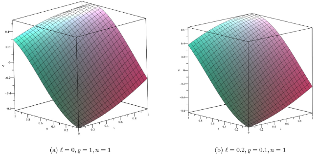
Fig. 18. Solution profile of distinct values of α in uncertain case for Example 4. |

Fig. 19. Solution profile for distinct values of α in crisp and uncertain case for Example 4. |
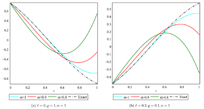
Fig. 20. Solution behaviour for distinct values of α in crisp and uncertain case for Example 4. |
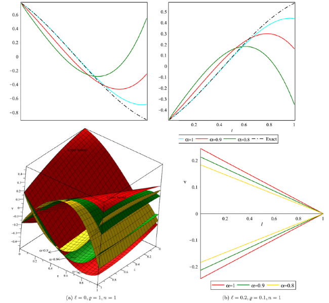
Fig. 21. Solution behaviour for distinct values of α in lower and upper bound for Example 4. |
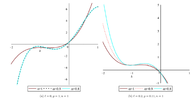
Fig. 22. Solution behaviour for distinct values of α in lower and upper bound for Example 4. |
6. Conclusion
This paper used two parameters based on the q-HAShTM for the non-linear FFKdVE under gH-differentiability of Caputo fractional-order via the ℓ-cut. In the presence of a fuzzy function, the convergence of the solution is checked numerically using the term approximations and theorems. The h-curve was used to validate the value of h required in the computation and find a suitable value of h that yields convergent and efficient solutions correlated to other available approaches. In addition, under gH-differentiability, the order of the fractional derivative affects the FFKdVE solution. Numerical results and comparisons showed that the proposed strategy is efficient and robust.
Declaration of Competing Interest
The authors declare that they have no conflict of interest.
Acknowledgements
The authors wish to express their sincere thanks to the Editor and the anonymous reviewers for carefully reading this manuscript and making many important suggestions, leading to a better presentation of the results.
