
1. Introduction
The NLPDEs are used to model many physical phenomena of real world and the most fundamental models are the studies of nonlinear phenomena. Such complicated physical phenomena arise in different fields of sciences, engineering, and many other fields such as aerospace industry, biology, plasma physics, nonlinear mechanics, meteorology, population ecology, and oceanography [1], [2], [3], [4], [5], [6], [7], [8], [9], [10], [11], [12], [13], [14], [15], [16], [17], [18], [19], [20], [21], [22], [23]. The exact solutions of NLPDEs will help to understand the phenomena in a better way. In last decade, numerous methods were applied to get the exact solutions of the NLPDEs such as the $\left(G^{\prime} / G\right)$-expansion method [24], the generalized Kudryashov method [25], the modified transformed rational function method [26], new modified extended direct algebraic [27], the soliton ansatz method [28] and many others [29], [30], [31], [32], [33], [34], [35], [36], [37], [38], [39], [40], [41], [42], [43].
There are different types of exact solutions and one of them is rational type solutions which includes lump, soliton, lump-kink, rogue-wave, and breather-wave solutions. A wide range of scholars are working to obtain such solutions. Lump solutions are nonsingular, real and decaying in all directions [44], [45], [46], [47]. It is widely used to describe the freak wave in the ocean [48], the nonlinear localized wave in plasma [49] and the rogue wave in Bose-Einstein condensate [50].
Moreover, the KdV equation is a NLPDE of third order. It was derived to model shallow-water waves with weak nonlinearity. The KdV equation possesses traveling wave solutions and a specific traveling wave solution is called soliton. It has many applications such as wave propagation in the water tanks, in the ocean, in the nonlinear optics, and in different plasma models, Wazwaz [51], Bulut et al. [52]. It is common in the early universe and in many space conditions to see electron-positron (EP) plasma. It occurs in active galactic nuclei, pulsar magnetospheres, accretion discs, neutron stars and cosmic solar flares. Black hole magnetospheres are also involved in the EP occurrence. EP plasmas have different physical properties than electron-ion plasma. Researchers examined the modulational instability of the wave equation for an ultra-intense, linearly polarized laser pulse traveling through EP plasma. We can expect some new physics conclusions from the magneto hydrodynamics of an electron-positron plasma compared to an electron-ion plasma [53]. The gKdV-ZK equations are an important models for numerous physical phenomena as well as waves in nonlinear LC circuit by way of mutual inductance among neighboring inductors, shallow and stratified internal waves, ion-acoustic waves in plasma physics, applications in space environments and astrophysical, nonlinear optic, hydrondynamic and many more. The higher dimensional gKdV-ZK equation is used in the infield of plasma physics which describes the effects of magnetic field on weak ion-acoustic wave [54]. The simplest model is that of ion-acoustic solitons, where the hot isothermal electrons are described by a Boltzmann distribution, while the cooler ions are treated as a fluid with adiabatic pressures [55]. The KdV-ZKe was established using multifluid equations in the literature [57].
Additionally, the shallow-water equations are a collection of hyperbolic partial differential equations that explain fluid flow beneath a pressure surface. Water wave dispersion refers to frequency dispersion in fluid dynamics, which means waves of different wavelengths travel at varying phase speeds. In this context, water waves are waves that propagate on the water’s surface, with gravity and surface tension acting as restoring forces. As a result, water with a free surface is commonly thought of as a dispersive medium. Ocean engineering involves the development, design, operation, and maintenance of watercraft propulsion and ocean systems using a variety of engineering sciences such as mechanical engineering, electrical engineering, electronic engineering, and computer science. Power and propulsion plants, machinery, piping, automation and control systems for all types of marine vehicles, as well as coastal and offshore constructions, are all included. Water wave equations describe various nonlinear physical phenomena in the above mentioned areas.
This paper is organized as fallows: In the Section 2, the governing equation, and in Section 3 extraction of solutions are presented. In the last section we discuss the conclusion.
2. Governing equation
$\Phi_{t}+\alpha \Phi^{2} \Phi_{x z}+\beta \Phi_{x x z x}+\nu\left(\Phi_{y y}+\Phi_{z z}\right)_{x}=0,$
where, $\Phi(x, y, z, t)$ is wave profile which is defined spatiotemporal variables in fluid icons, with $α,β$, and $ν$ are real constants that govern the oblique distribution of non-linear electrostatic modes which describes mixtures of hot isothermal, warm adiabatic fluid, and cold immobile background species [55]. In the next section, we discuss the different wave structures by using the proposed techniques. The governing equation which is an important model arises in different branches of physics such as plasma physics, nonlinear optics, fluid dynamics, theoretical physics quantum mechanics and mathematical physics to analize the main properties of non-linear propagation of various physical phenomena. All of our results are vital for comprehending nonlinear phenomena in dispersive waves, which are relevant to ocean engineering and plasma physics. By examining the interaction solutions to the examined model in nonlinear dispersive waves, other researchers will be able to do additional research on the effects of dispersive waves on coastal processes and the interactions of waves with complex structures in near shore locations. The mathematical modeling of tsunamis and tidal oscillations can be used as an example to utilize this studied equation in ocean engineering. These kinds of equations can also be used in engineering, such as in the prediction of refraction, atness, and harmonic interactions near coastal constructions.
3. Diversity of wave structures
For discussing the studied model, we use the transformation $\Phi(x, y, z, t)=P(\xi)$, where $\xi=x+y+z-c t$, in Eq. (1), and get the ordinary differential equation as follows:
$-c P^{\prime}+\alpha P^{2} P^{\prime}+(\beta+2 \nu) P^{\prime \prime \prime}=0$
Now, integrate Eq. (2) w.r.t ξ to reduce the order of ODE and we get the following form as:
$-c P+\alpha \frac{P^{3}}{3}+(\beta+2 \nu) P^{\prime \prime}=0$
Now, our concern is to deal the Eq. (3).
3.1. $\phi^{6}$-model expansion method [56]
In this subsection, by the assistance of $\phi^{6}$-model expansion method, we secure the different solutions. The solution of Eq. (3) on taking $n=1$ is expressed as:
$P(\xi)=\zeta_{0}+\zeta_{1} \varrho+\zeta_{2} \varrho^{2} \text {, }$
where $\zeta_{0}, \zeta_{1}, \zeta_{2}$ are constants to be determined later. Manipulating the Eqs. (4) and (3) together and adopting the method, we get
Family-1.
$\left\{\begin{array}{l} \zeta_{0}=\zeta_{0}, \zeta_{1}=0, \zeta_{2}=\zeta_{2} \chi_{0}=-\frac{\zeta_{0}\left(\alpha \zeta_{0}^{2}-3 c\right)}{6 \zeta_{2}(\beta+2 \nu)} \\ \chi_{2}=\frac{c-\alpha \zeta_{0}^{2}}{4(\beta+2 \nu)}, \chi_{4}=-\frac{\alpha \zeta_{0} \zeta_{2}}{6(\beta+2 \nu)}, \chi_{6}=-\frac{\alpha \zeta_{2}^{2}}{24(\beta+2 \nu)} \end{array}\right.$
3.1.1. Jacobi elliptic function and soliton solutions
The solutions of Eq. (3), and consequently Eq. (1), corresponding to Family-1 are calculated as:
1. If $l_{0}=1, l_{2}=-\left(1+m^{2}\right), l_{4}=m^{2}, 0<m<1$, then $\Theta(\xi)=\operatorname{sn}(\xi, m)$ or $\Theta(\xi)=\operatorname{cd}(\xi, m)$, retrieve JEF solution
$\Phi_{1}(x, y, z, t)=\frac{\zeta_{2} \operatorname{sn}(\xi, m)^{2}}{f \operatorname{sn}(\xi, m)^{2}+g}+\zeta_{0}$
or
$\Phi_{2}(x, y, z, t)=\frac{\zeta_{2} \operatorname{cd}(\xi, m)^{2}}{f \operatorname{cd}(\xi, m)^{2}+g}+\zeta_{0}$
where
$\begin{array}{l} f=\frac{2 \alpha \zeta_{0} \zeta_{2}\left(-\alpha \zeta_{0}^{2}+c+4\left(m^{2}+1\right)(\beta+2 \nu)\right)}{3\left(\alpha^{2} \zeta_{0}^{4}+c^{2}-2 \alpha c \zeta_{0}^{2}-16\left(m^{4}-m^{2}+1\right)(\beta+2 \nu)^{2}\right)} \\ g=-\frac{8 \alpha \zeta_{0} \zeta_{2}(\beta+2 \nu)}{\alpha^{2} \zeta_{0}^{4}+c^{2}-2 \alpha c \zeta_{0}^{2}-16\left(m^{4}-m^{2}+1\right)(\beta+2 \nu)^{2}} \end{array}$
under the constraints condition
$\begin{array}{c} \frac{\alpha^{2} \zeta_{0}^{2} \zeta_{2}^{2}\left(-\frac{c-\alpha S_{0}^{2}}{4 \beta+8 \nu}-m^{2}-1\right)\left(9 m^{2}-\frac{\left(-\alpha S_{0}^{2}+c+4\left(m^{2}+1\right)(\beta+2 \nu)\right)\left(\alpha \zeta_{0}^{2}-c+8\left(m^{3}+1\right)(\beta+2 \nu)\right)}{16(\beta+2 \nu)^{2}}\right)}{36(\beta+2 \nu)^{2}} \\ \quad+3\left(\left(-\frac{\alpha \zeta_{2}^{2}}{24(\beta+2 \nu)}\right)\left(\frac{\left(c-\alpha \zeta_{0}^{2}\right)^{2}}{16(\beta+2 \nu)^{2}}+3 m^{2}-\left(m^{2}+1\right)^{2}\right)\right)^{2}=0 \end{array}$
Remarks :
•On choosing $m \rightarrow 1$ in Eq. (5), the soliton solutions are mentioned as:
$\begin{array}{l} \Phi_{1,1}(x, y, z, t) \\ \quad \tanh ^{2}(\xi)\left(-\alpha^{2} \zeta_{0}^{4}-3(4 \beta+c+8 \nu)(c-4(\beta+2 \nu))\right) \\ \quad+2 \alpha \zeta_{0}^{2} \operatorname{sech}^{2}(\xi)(10(\beta+2 \nu)+\cosh (2 \xi)(2 \beta+c+4 \nu) \\ =\frac{-c)}{2 \alpha \zeta_{0}\left(12(\beta+2 \nu)-\tanh ^{2}(\xi)\left(-\alpha \zeta_{0}^{2}+8(\beta+2 \nu)+c\right)\right)} \end{array}$
provided that
$\begin{array}{l} \frac{\alpha^{2} \zeta_{0}^{2} \zeta_{2}^{2}\left(-\frac{c-\alpha \zeta_{0}^{2}}{4 \beta+8 \nu}-2\right)\left(\frac{\left(\alpha \zeta_{0}^{2}+4 \beta-c+8 \nu\right)^{2}}{16(\beta+2 \nu)^{2}}\right)}{\beta+2 \nu} \\ +108(\beta+2 \nu)\left(\left(-\frac{\alpha \zeta_{2}^{2}}{24(\beta+2 \nu)}\right)\left(\frac{\left(c-\alpha \zeta_{0}^{2}\right)^{2}}{16(\beta+2 \nu)^{2}}-1\right)\right)^{2}=0=0 \end{array}$
•On choosing $m \rightarrow 01$ in Eq. (7), the periodic solutions are expressed as:
$\begin{array}{l} \begin{array}{l} \Phi_{2,1}(x, y, z, t) \\ \alpha^{2} \zeta_{0}^{4} \cos ^{2}(\xi)+3 \cos ^{2}(\xi)\left(c^{2}-16(\beta+2 \nu)^{2}\right) \\ =\frac{-2 \alpha \zeta_{0}^{2}(10(\beta+2 \nu)+\cos (2 \xi)(c-2(\beta+2 \nu))+c)}{2 \alpha \zeta_{0}\left(-\alpha \zeta_{0}^{2} \cos ^{2}(\xi)-8(\beta+2 \nu)\right.}, \\ \left.+\sin ^{2}(\xi)(-(4 \beta+c+8 \nu))+c\right) \end{array}\\ \Phi_{2,1}(x, y, z, t)\\ \alpha^{2} \zeta_{0}^{4} \cos ^{2}(\xi)+3 \cos ^{2}(\xi)\left(c^{2}-16(\beta+2 \nu)^{2}\right)\\ =\frac{-2 \alpha \zeta_{0}^{2}(10(\beta+2 \nu)+\cos (2 \xi)(c-2(\beta+2 \nu))+c)}{2 \alpha \zeta_{0}\left(-\alpha \zeta_{0}^{2} \cos ^{2}(\xi)-8(\beta+2 \nu)\right.},\\ \left.+\sin ^{2}(\xi)(-(4 \beta+c+8 \nu))+c\right) \end{array}$
provided that
$\begin{array}{l} \frac{\alpha^{2} \zeta_{0}^{2} \zeta_{2}^{2}\left(-\frac{c-\alpha \varsigma_{0}^{2}}{4 \beta+8 \nu}-1\right)\left(\frac{\left(-\alpha \varsigma_{0}^{2}+4 \beta+c+8 \nu\right)\left(-\alpha \zeta_{0}^{2}-8(\beta+2 \nu)+c\right)}{16(\beta+2 \nu)^{2}}\right)}{36(\beta+2 \nu)^{2}} \\ +3\left(\left(-\frac{\alpha \zeta_{2}^{2}}{24(\beta+2 \nu)}\right)\left(\frac{\left(c-\alpha \zeta_{0}^{2}\right)^{2}}{16(\beta+2 \nu)^{2}}-1\right)\right)^{2}=0 \end{array}$
where, $\xi=x+y+z-c t$.
2. If $l_{0}=1-m^{2}, l_{2}=2 m^{2}-1, l_{4}=-m^{2}, 0<m<1$, then $\Theta(\xi)=\operatorname{cn}(\xi, m)$, provides JEF solution
$\Phi_{3}(x, y, z, t)=\frac{\zeta_{2} \operatorname{cn}(\xi, m)^{2}}{f \operatorname{cn}(\xi, m)^{2}+g}+\zeta_{0}$
Where
$\begin{aligned} f & =\frac{2 \alpha \zeta_{0} \zeta_{2}\left(-\alpha \zeta_{0}^{2}+c-4\left(2 m^{2}-1\right)(\beta+2 \nu)\right)}{3\left(\alpha^{2} \zeta_{0}^{4}+c^{2}-2 \alpha c \zeta_{0}^{2}-16\left(m^{4}-m^{2}+1\right)(\beta+2 \nu)^{2}\right)} \\ g & =\frac{8 \alpha \zeta_{0} \zeta_{2}\left(m^{2}-1\right)(\beta+2 \nu)}{\alpha^{2} \zeta_{0}^{4}+c^{2}-2 \alpha c \zeta_{0}^{2}-16\left(m^{4}-m^{2}+1\right)(\beta+2 \nu)^{2}} \end{aligned}$
under the constraints condition
$\begin{array}{l} \begin{array}{l} \frac{\alpha^{2} \zeta_{0}^{2} \zeta_{2}^{2}\left(-\frac{c-\alpha \zeta_{0}^{2}}{4 \beta+8 \nu}+2 m^{2}-1\right)\left(\frac{\left(-\alpha \zeta_{0}^{2}+c+4\left(m^{2}-2\right)(\beta+2 \nu)\right)\left(-\alpha \zeta_{0}^{2}+c+4\left(m^{2}+1\right)(\beta+2 \nu)\right)}{16(\beta+2 \nu)^{2}}\right)}{36(\beta+2 \nu)^{2}} \\ +3\left(\left(-\frac{\alpha \zeta_{2}^{2}}{24(\beta+2 \nu)}\right)\left(\frac{\left(c-\alpha \zeta_{0}^{2}\right)^{2}}{16(\beta+2 \nu)^{2}}+3\left(m^{2}-1\right) m^{2}-\left(1-2 m^{2}\right)^{2}\right)\right)^{2}=0. \end{array}\\ \frac{\alpha^{2} \zeta_{0}^{2} \zeta_{2}^{2}\left(-\frac{c-\alpha \zeta_{0}^{2}}{4 \beta+8 \nu}+2 m^{2}-1\right)\left(\frac{\left(-\alpha \zeta_{0}^{2}+c+4\left(m^{2}-2\right)(\beta+2 \nu)\right)\left(-\alpha \zeta_{0}^{2}+c+4\left(m^{2}+1\right)(\beta+2 \nu)\right)}{16(\beta+2 \nu)^{2}}\right)}{36(\beta+2 \nu)^{2}}\\ +3\left(\left(-\frac{\alpha \zeta_{2}^{2}}{24(\beta+2 \nu)}\right)\left(\frac{\left(c-\alpha \zeta_{0}^{2}\right)^{2}}{16(\beta+2 \nu)^{2}}+3\left(m^{2}-1\right) m^{2}-\left(1-2 m^{2}\right)^{2}\right)\right)^{2}=0. \end{array}$
where,$ \xi=x+y+z-c t$.
3. If $l_{0}=m^{2}-1, l_{2}=2-m^{2}, l_{4}=-1,0<m<1$, then $\Theta(\xi)=\operatorname{dn}(\xi, m)$, gives JEF solution
$\Phi_{4}(x, y, z, t)=\frac{\zeta_{2} \operatorname{dn}(\xi, m)^{2}}{f \operatorname{dn}(\xi, m)^{2}+g}+\zeta_{0}$
Where
$\begin{array}{r} f=\frac{2 \alpha \zeta_{0} \zeta_{2}\left(-\alpha \zeta_{0}^{2}+c+4\left(m^{2}-2\right)(\beta+2 \nu)\right)}{3\left(\alpha^{2} \zeta_{0}^{4}+c^{2}-2 \alpha c \zeta_{0}^{2}-16\left(m^{4}-m^{2}+1\right)(\beta+2 \nu)^{2}\right)} \\ g=-\frac{8 \alpha \zeta_{0} \zeta_{2}\left(m^{2}-1\right)(\beta+2 \nu)}{\alpha^{2} \zeta_{0}^{4}+c^{2}-2 \alpha c \zeta_{0}^{2}-16\left(m^{4}-m^{2}+1\right)(\beta+2 \nu)^{2}} \end{array}$
under the constraints condition
$\frac{\alpha^{2} \zeta_{0}^{2} \zeta_{2}^{2}\left(-\frac{c-\alpha \zeta_{0}^{2}}{4 \beta+8 \nu}-m^{2}+2\right)\left(\frac{\left(-\alpha \zeta_{0}^{2}+c+4\left(m^{2}-2\right)(\beta+2 \nu)\right)\left(-\alpha \zeta_{0}^{2}+c-8\left(m^{2}-2\right)(\beta+2 \nu)\right)}{16(\beta+2 \nu)^{2}}-9 m^{2}\right. +9)}{\quad+3\left(\left(-\frac{\alpha \zeta_{2}^{2}}{24(\beta+2 \nu)}\right)\left(\frac{\left(c-\alpha \zeta_{0}^{2}\right)^{2}}{16(\beta+2 \nu)^{2}}-3 m^{2}-\left(m^{2}-2\right)^{2}+3\right)\right)^{2}=0}$
4.If $l_{0}=m^{2}, l_{2}=-\left(1+m^{2}\right), l_{4}=1,0<m<1$, then $\Theta(\xi)=\mathrm{ns}(\xi, m)$, provide JEF solution
$\Phi_{5}(x, y, z, t)=\frac{\zeta_{2} \mathrm{~ns}(\xi, m)^{2}}{f \mathrm{~ns}(\xi, m)^{2}+g}+\zeta_{0}$
where
$\begin{array}{r} f=\frac{2 \alpha \zeta_{0} \zeta_{2}\left(-\alpha \zeta_{0}^{2}+c+4\left(m^{2}+1\right)(\beta+2 \nu)\right)}{3\left(\alpha^{2} \zeta_{0}^{4}+c^{2}-2 \alpha c \zeta_{0}^{2}-16\left(m^{4}-m^{2}+1\right)(\beta+2 \nu)^{2}\right)} \\ g=-\frac{8 \alpha \zeta_{0} \zeta_{2} m^{2}(\beta+2 \nu)}{\alpha^{2} \zeta_{0}^{4}+c^{2}-2 \alpha c \zeta_{0}^{2}-16\left(m^{4}-m^{2}+1\right)(\beta+2 \nu)^{2}} \end{array}$
under the constraints condition
$\begin{array}{l} \frac{\alpha^{2} \zeta_{0}^{2} \zeta_{2}^{2}\left(-\frac{c-\alpha \varsigma_{0}^{2}}{4 \beta+8 \nu}-m^{2}-1\right)\left(9 m^{2}-\frac{\left(-\alpha \zeta_{0}^{2}+c+4\left(m^{2}+1\right)(\beta+2 \nu)\right)\left(\alpha \zeta_{0}^{2}-c+8\left(m^{2}+1\right)(\beta+2 \nu)\right)}{16(\beta+2 \nu)^{2}}\right)}{36(\beta+2 \nu)^{2}} \\ \quad+3\left(\left(-\frac{\alpha \zeta_{2}^{2}}{24(\beta+2 \nu)}\right)\left(\frac{\left(c-\alpha \zeta_{0}^{2}\right)^{2}}{16(\beta+2 \nu)^{2}}+3 m^{2}-\left(m^{2}+1\right)^{2}\right)\right)^{2}=0 \end{array}$
Remark :
•On selecting m→1 in Eq. (11), we extract explicit solitary solutions as:
$\begin{array}{l} \Phi_{5,1}(x, y, z, t) \\ \quad-\alpha^{2} \zeta_{0}^{4} \operatorname{coth}^{2}(\xi)+3 \operatorname{coth}^{2}(\xi)\left(208(\beta+2 \nu)^{2}-c^{2}\right) \\ =\frac{+4 \alpha \zeta_{0}^{2}\left(6(\beta+2 \nu)+\operatorname{coth}^{2}(\xi)(c-8(\beta+2 \nu))\right)}{2 \alpha \zeta_{0}\left(\alpha \zeta_{0}^{2} \operatorname{coth}^{2}(\xi)+12(\beta+2 \nu)-\operatorname{coth}^{2}(\xi)(16 \beta+c+32 \nu)\right)} \end{array}$
provided that
$\begin{aligned} \frac{\alpha^{2} \zeta_{0}^{2} \zeta_{2}^{2}\left(-\frac{c-\alpha S_{0}^{2}}{4 \beta+8 \nu}-4\right)\left(\frac{\left(-\alpha \zeta_{0}^{2}+16 \beta+c+32 \nu\right)\left(-\alpha \zeta_{0}^{2}-32(\beta+2 \nu)+c\right)}{16(\beta+2 \nu)^{2}}+9\right)}{36(\beta+2 \nu)^{2}} \\ +3\left(\left(-\frac{\alpha \zeta_{2}^{2}}{24(\beta+2 \nu)}\right)\left(\frac{\left(c-\alpha \zeta_{0}^{2}\right)^{2}}{16(\beta+2 \nu)^{2}}-13\right)\right)^{2}=0 \end{aligned}$
where, $\xi=x+y+z-c t \mid$.
5. If $l_{0}=-m^{2}, l_{2}=-1+2 m^{2}, l_{4}=1-m^{2}, 0<m<1$, then $\Theta(\xi)=\operatorname{nc}(\xi, m)$, reveals JEF solution
$\Phi_{6}(x, y, z, t)=\frac{\zeta_{2} \mathrm{nc}(\xi, m)^{2}}{f \mathrm{nc}(\xi, m)^{2}+g}+\zeta_{0}$
where
$\begin{array}{c} f=\frac{2 \alpha \zeta_{0} \zeta_{2}\left(-\alpha \zeta_{0}^{2}+c-4\left(2 m^{2}-1\right)(\beta+2 \nu)\right)}{3\left(\alpha^{2} \zeta_{0}^{4}+c^{2}-2 \alpha c \zeta_{0}^{2}-16\left(m^{4}-m^{2}+1\right)(\beta+2 \nu)^{2}\right)} \\ g=\frac{8 \alpha \zeta_{0} \zeta_{2} m^{2}(\beta+2 \nu)}{\alpha^{2} \zeta_{0}^{4}+c^{2}-2 \alpha c \zeta_{0}^{2}-16\left(m^{4}-m^{2}+1\right)(\beta+2 \nu)^{2}} \end{array}$
under the constraints condition
$\begin{array}{l} \frac{\alpha^{2} \zeta_{0}^{2} \zeta_{2}^{2}\left(-\frac{c-\alpha \zeta_{0}^{2}}{4 \beta+8 \nu}+2 m^{2}-1\right)\left(\frac{\left(-\alpha \zeta_{0}^{2}+c+4\left(m^{2}-2\right)(\beta+2 \nu)\right)\left(-\alpha S_{0}^{2}+c+4\left(m^{2}+1\right)(\beta+2 \nu)\right)}{16(\beta+2 \nu)^{2}}\right)}{36(\beta+2 \nu)^{2}} \\ +3\left(\left(-\frac{\alpha \zeta_{2}^{2}}{24(\beta+2 \nu)}\right)\left(\frac{\left(c-\alpha \zeta_{0}^{2}\right)^{2}}{16(\beta+2 \nu)^{2}}+3\left(m^{2}-1\right) m^{2}-\left(1-2 m^{2}\right)^{2}\right)\right)^{2} \\ =0 \text {, } \end{array}$
Remark :
On choosing m→1 in Eq. (13), solution in hyperbolic form is written as:
$\begin{array}{l} \Phi_{6,1}(x, y, z, t) \\ \quad-\alpha^{2} \zeta_{0}^{4} \cosh ^{2}(\xi)+3 \cosh ^{2}(\xi)\left(16(\beta+2 \nu)^{2}-c^{2}\right) \\ =\frac{+2 \alpha \zeta_{0}^{2}(-10(\beta+2 \nu)+\cosh (2 \xi)(2 \beta+c+4 \nu)+c)}{2 \alpha \zeta_{0}\left(\alpha \zeta_{0}^{2} \cosh ^{2}(\xi)-12(\beta+2 \nu)+\cosh ^{2}(\xi)(4 \beta-c+8 \nu)\right)} \end{array}$
provided that
$\begin{array}{l} -\frac{\alpha^{2} \zeta_{0}^{2} \zeta_{2}^{2}\left(1-\frac{c-\alpha \zeta_{0}^{2}}{4 \beta+8 \nu}\right)\left(-\frac{\left(-\alpha \zeta_{0}^{2}+8 \beta+c+16 \nu\right)\left(\alpha \zeta_{0}^{2}+4 \beta-c+8 \nu\right)}{16(\beta+2 \nu)^{2}}\right)}{36(\beta+2 \nu)^{2}} \\ +3\left(\left(-\frac{\alpha \zeta_{2}^{2}}{24(\beta+2 \nu)}\right)\left(\frac{\left(c-\alpha \zeta_{0}^{2}\right)^{2}}{16(\beta+2 \nu)^{2}}-1\right)\right)^{2}=0 \end{array}$
where, $\xi=x+y+z-c t$.
6. If $l_{0}=1, l_{2}=2-m^{2}, l_{4}=1-m^{2}, 0<m<1$, then $\Theta(\xi)=\mathrm{sc}(\xi, m)$, retrieve JEF solution
$\Phi_{7}(x, y, z, t)=\frac{\zeta_{2} \operatorname{sc}(\xi, m)^{2}}{f \mathrm{sc}(\xi, m)^{2}+g}+\zeta_{0}$
Where
$\begin{array}{r} f=\frac{2 \alpha \zeta_{0} \zeta_{2}\left(-\alpha \zeta_{0}^{2}+c+4\left(m^{2}-2\right)(\beta+2 \nu)\right)}{3\left(\alpha^{2} \zeta_{0}^{4}+c^{2}-2 \alpha c \zeta_{0}^{2}-16\left(m^{4}-m^{2}+1\right)(\beta+2 \nu)^{2}\right)} \\ g=-\frac{8 \alpha \zeta_{0} \zeta_{2}(\beta+2 \nu)}{\alpha^{2} \zeta_{0}^{4}+c^{2}-2 \alpha c \zeta_{0}^{2}-16\left(m^{4}-m^{2}+1\right)(\beta+2 \nu)^{2}} \end{array}$
under the constraints condition
$\begin{array}{l} \alpha^{2} \zeta_{0}^{2} \zeta_{2}^{2}\left(-\frac{c-\alpha \zeta_{0}^{2}}{4 \beta+8 \nu}-m^{2}+2\right)\left(\frac{\left(-\alpha \zeta_{0}^{2}+c+4\left(m^{2}-2\right)(\beta+2 \nu)\right)\left(-\alpha \zeta_{\left.L_{2}^{2}+c-8\left(m^{2}-2\right)(\beta+2 \nu)\right)}^{16(\beta+2 \nu)^{2}}-9 m^{2}\right.}{+9)}\right. \\ \quad+3\left(\left(-\frac{\alpha \zeta_{2}^{2}}{24(\beta+2 \nu)}\right)\left(\frac{\left(c-\alpha \zeta_{0}^{2}\right)^{2}}{16(\beta+2 \nu)^{2}}-3 m^{2}-\left(m^{2}-2\right)^{2}+3\right)\right)^{2}=0 \end{array}$
Remarks :
•On taking m→1 in Eq. (15), we get the following solitary solution as:
$\begin{array}{l} \Phi_{7,1}(x, y, z, t) \\ -\alpha^{2} \zeta_{0}^{4} \sinh ^{2}(\xi)+3 \sinh ^{2}(\xi)\left(16(\beta+2 \nu)^{2}-c^{2}\right) \\ =\frac{+2 \alpha \zeta_{0}^{2}(10(\beta+2 \nu)+\cosh (2 \xi)(2 \beta+c+4 \nu)-c)}{\alpha \zeta_{0}\left(2 \alpha \zeta_{0}^{2} \sinh ^{2}(\xi)+20 \beta+\cosh (2 \xi)(4 \beta-c+8 \nu)\right.}, \\ +c+40 \nu) \end{array}$
provided that
$\frac{\alpha^{2} \zeta_{0}^{2} \zeta_{2}^{2}\left(1-\frac{c-\alpha \zeta_{0}^{2}}{4 \beta+8 v}\right)\left(-\frac{\left(-\alpha \zeta_{0}^{2}+8 \beta+c+16 v\right)\left(\alpha \zeta_{5}^{2}+4 \beta-c+8 v\right)}{16(\beta+2 v)^{2}}\right)}{36(\beta+2 v)^{2}}+3\left(\left(-\frac{\alpha \zeta_{2}^{2}}{24(\beta+2 v)}\right)\left(\frac{\left(c-\alpha \zeta_{0}^{2}\right)^{2}}{16(\beta+2 v)^{2}}-1\right)\right)^{2}=0$
•On considering m→0 in Eq. (15), periodic solutions are obtained as:
$\Phi_{7,2}(x, y, z, t)=-\frac{\alpha^{2} \zeta_{0}^{4} \tan ^{2}(\xi)+3 \tan ^{2}(\xi)\left(c^{2}-16(\beta+2 v)^{2}\right)+2 \alpha \zeta_{0}^{2} \sec ^{2}(\xi)(-10(\beta+2 v)+\cos (2 \xi)(c-2(\beta+2 v))-c)}{2 \alpha \zeta_{0}\left(\alpha \zeta_{0}^{2} \tan ^{2}(\xi)+4 \beta+\sec ^{2}(\xi)(8 \beta-c+16 v)+c+8 v\right)} $
provided that
$\frac{\alpha^{2} \zeta_{0}^{2} \zeta_{2}^{2}\left(2-\frac{c-\alpha \zeta_{0}^{2}}{4 \beta+8 v}\right)\left(\frac{\left(-\alpha \zeta_{0}^{2}+4 \beta+c+8 v\right)^{2}}{16(\beta+2 v)^{2}}\right)}{36(\beta+2 v)^{2}}+3\left(\left(-\frac{\alpha \zeta_{2}^{2}}{24(\beta+2 v)}\right)\left(\frac{\left(c-\alpha \zeta_{0}^{2}\right)^{2}}{16(\beta+2 v)^{2}}-1\right)\right)^{2}=0$
where, $\xi=x+y+z-c t$.
7. If $l_{0}=\frac{1}{4}, l_{2}=\frac{1-2 m^{2}}{2}, l_{4}=\frac{1}{4}, 0<m<1$, then $\Theta(\xi)=\frac{\operatorname{sn}(\xi, m)}{1 \pm \operatorname{cn}(\eta, m)}$, gives JEF solution
$\Phi_{8}(x, y, z, t)=\frac{\zeta_{2} \operatorname{sn}(\xi, m)^{2}}{g(1 \pm \operatorname{cn}(\xi, m))^{2}+f \operatorname{sn}(\xi, m)^{2}}+\zeta_{0}$
Remarks :
•On selecting m→1 in Eq. (15), combined bright-dark soliton solutions are achieved as:
$\Phi_{8,1}(x, y, z, t)=\frac{6 \alpha \zeta_{0}^{2}(\beta+2 v)(1 \pm \operatorname{sech}(\xi))^{2}+\tanh ^{2}(\xi)\left(-\alpha^{2} \zeta_{0}^{4}+3\left((\beta+2 v)^{2}-c^{2}\right)+4 \alpha \zeta_{0}^{2}(-\beta+c-2 v)\right)}{2 \alpha \zeta_{0}\left(3(\beta+2 v)(1 \pm \operatorname{sech}(\xi))^{2}-\tanh ^{2}(\xi)\left(-\alpha \zeta_{0}^{2}+2 \beta+c+4 v\right)\right)}$
provided that
$\frac{\alpha^{2} \zeta_{0}^{2} \zeta_{2}^{2}\left(-\frac{c-\alpha \zeta_{0}^{2}}{4 \beta+8 v}-\frac{1}{2}\right)\left(\frac{\left(\alpha \zeta_{0}^{2}+\beta-c+2 v\right)^{2}}{16(\beta+2 v)^{2}}\right)}{36(\beta+2 v)^{2}}+3\left(\left(-\frac{\alpha \zeta_{2}^{2}}{24(\beta+2 v)}\right)\left(\frac{1}{16}\left(\frac{\left(c-\alpha \zeta_{0}^{2}\right)^{2}}{(\beta+2 v)^{2}}-1\right)\right)\right)^{2}=0$
•On choosing m→0 in Eq. (15), we obtain solution as:
$\Phi_{8,2}(x, y, z, t)=\frac{6 \alpha \zeta_{0}^{2}(\beta+2 v)(1 \pm \cos (\xi))^{2}+\sin ^{2}(\xi)\left(-\alpha^{2} \zeta_{0}^{4}+3\left((\beta+2 v)^{2}-c^{2}\right)+4 \alpha \zeta_{0}^{2}(\beta+c+2 v)\right)}{2 \alpha \zeta_{0}\left(3(\beta+2 v)(1 \pm \cos (\xi))^{2}+\sin ^{2}(\xi)\left(\alpha \zeta_{0}^{2}+2 \beta-c+4 v\right)\right)}$
provided that
$\frac{\alpha^{2} \zeta_{0}^{2} \zeta_{2}^{2}\left(\frac{1}{2}-\frac{c-\alpha \zeta_{0}^{2}}{4 \beta+8 v}\right)\left(\frac{\left(-\alpha \zeta_{0}^{2}+\beta+c+2 v\right)^{2}}{16(\beta+2 v)^{2}}\right)}{36(\beta+2 v)^{2}}+3\left(\left(-\frac{\alpha \zeta_{2}^{2}}{24(\beta+2 v)}\right)\left(\frac{1}{16}\left(\frac{\left(c-\alpha \zeta_{0}^{2}\right)^{2}}{(\beta+2 v)^{2}}-1\right)\right)\right)^{2}=0$
where, $\xi=x+y+z-c t$. The graphical view of some of the above earned solutions are depicted below as:
3.2. Interaction aspects
$P=(\ln f)_{\xi}$
Substitute Eq. (21) in Eq. (3) and get the bilinear form as,
$(\alpha+6(\beta+2 \nu)) f_{\xi}^{3}-9(\beta+2 \nu) f f_{\xi} f_{\xi \xi}-3 c f^{2} f_{\xi}+3(\beta+2 \nu) f^{2} f_{\xi \xi \xi}=0$
In this next sections, we find the different wave structures of gKdV-ZK, such as three wave hypothesis, breather wave, lump periodic, mixed type wave solutions, and periodic cross kink.
•MultiwaveSolutions:
We extract different forms of solutions by using the three wave hypothesis with the assistance of the following transformation [63] as:
$f=\kappa_{0} \cosh \left(\delta_{1} \xi+\delta_{2}\right)+\kappa_{1} \cos \left(\delta_{3} \xi+\delta_{4}\right)+\kappa_{2} \cosh \left(\delta_{5} \xi+\delta_{6}\right)$
where, $\kappa_{i}(i=1,2,3)$ and $\delta_{j} \mid(j=1,2 \ldots, 6)$ are the real constant that are determine later. Substitute Eq. (23) in Eq. (22) using its derivatives and after collecting all the coefficients of hyperbolic and trigonometric functions. So, we obtain the different sets of values of some parameters as:
Family 1:$ \kappa_{0}=\kappa_{0}, \kappa_{1}=\kappa_{1}, \kappa_{2}=0, \delta_{1}=\delta_{1}, \delta_{2}=\delta_{2}, \delta_{3}=-i \delta_{1}, \alpha=\frac{3 c}{\delta_{1}^{2}}$, and $\beta=\frac{-c-4 \delta_{1}^{2} \nu}{2 \delta_{1}^{2}}$, substitute these values in Eq. (23) then put in Eq. (21) and get the solution of Eq. (3) as,
$P(\xi)=\frac{\delta_{1} \kappa_{0} \sinh \left(\delta_{1} \xi+\delta_{2}\right)+\delta_{1} \kappa_{1} \sinh \left(\delta_{1} \xi+i \delta_{4}\right)}{\kappa_{0} \cosh \left(\delta_{1} \xi+\delta_{2}\right)+\kappa_{1} \cosh \left(\delta_{1} \xi+i \delta_{4}\right)}$
so the solution of Eq. (1) is obtained as:
$\Phi_{1}(x, y, z, t)=\frac{\delta_{1}\left(\kappa_{0} \sinh \left(\delta_{1}(\xi)+\delta_{2}\right)+\kappa_{1} \sinh \left(\delta_{1}(\xi)+i \delta_{4}\right)\right)}{\kappa_{0} \cosh \left(\delta_{1}(\xi)+\delta_{2}\right)+\kappa_{1} \cosh \left(\delta_{1}(\xi)+i \delta_{4}\right)}$
Family 2: $\delta_{1}=-i \delta_{3}, \delta_{2}=\delta_{2}, \delta_{3}=\delta_{3}, \delta_{4}=\delta_{4}, \delta_{5}=-i \delta_{3}, \alpha=-\frac{3 c}{\delta_{3}^{2}}$, and $\beta=\frac{c-4 \delta_{3}^{2} \nu}{2 \delta_{3}^{2}}$, substitute these values in Eq. (23) then put in Eq. (21) and the solution of Eq. (3) as:
$P(\xi)=\frac{i \delta_{3} \kappa_{0} \sinh \left(\delta_{2}+i \delta_{3} \xi\right)-\delta_{3} \kappa_{2} \sin \left(\delta_{3} \xi+i \delta_{6}\right)}{\kappa_{2} \cos \left(\delta_{3} \xi+i \delta_{6}\right)+\kappa_{0} \cosh \left(\delta_{2}+i \delta_{3} \xi\right)}$
So, the solution of Eq. (1) is obtained as:
$\Phi_{2}(x, y, z, t)=\frac{\delta_{3}\left(i \kappa_{0} \sinh \left(\delta_{2}+i \delta_{3}(\xi)\right)-\kappa_{2} \sin \left(\delta_{3}(\xi)+i \delta_{6}\right)\right)}{\kappa_{2} \cos \left(\delta_{3}(\xi)+i \delta_{6}\right)+\kappa_{0} \cosh \left(\delta_{2}+i \delta_{3}(\xi)\right)}$
Family 3: $\delta_{1}=\delta_{5}, \delta_{2}=\delta_{2}, \delta_{3}=-i \delta_{5}, \delta_{4}=\delta_{4}, \delta_{5}=\delta_{5}, \alpha=\frac{3 c}{\delta_{5}^{2}}$, and $\nu=\frac{-2 \beta \delta_{5}^{2}-c}{4 \delta_{5}^{2}}$2, substitute these values in Eq. (23) then put in Eq. (21) and the solution of Eq. (3) as:
$P(\xi)=\frac{i \delta_{5} \kappa_{1} \sin \left(\delta_{4}-i \delta_{5} \xi\right)+\delta_{5} \kappa_{0} \sinh \left(\delta_{5} \xi+\delta_{2}\right)+\delta_{5} \kappa_{2} \sinh \left(\delta_{5} \xi+\delta_{6}\right)}{\kappa_{1} \cos \left(\delta_{4}-i \delta_{5} \xi\right)+\kappa_{0} \cosh \left(\delta_{5} \xi+\delta_{2}\right)+\kappa_{2} \cosh \left(\delta_{5} \xi+\delta_{6}\right)}$
So, the solution of Eq. (1) is obtained as:
$\begin{array}{l} \Phi_{3}(x, y, z, t) \\ =\frac{\delta_{5}\left(i \kappa_{1} \sin \left(\delta_{4}-i \delta_{5} \xi\right)+\kappa_{0} \sinh \left(\delta_{5} \xi+\delta_{2}\right)+\kappa_{2} \sinh \left(\delta_{5} \xi+\delta_{6}\right)\right)}{\kappa_{1} \cos \left(\delta_{4}-i \delta_{5} \xi\right)+\kappa_{0} \cosh \left(\delta_{5} \xi+\delta_{2}\right)+\kappa_{2} \cosh \left(\delta_{5} \xi+\delta_{6}\right)} \end{array}$
where $\xi=x+y+z-c t$.
•Interactionviadoubleexponentialform:
We proceed by taking the following test function [64] as:
Let
$f=\kappa_{1} \exp \left(\delta_{1} \xi+\delta_{2}\right)+\kappa_{2} \exp \left(\delta_{3} \xi+\delta_{4}\right)$
where $\delta_{1}, \ldots, \delta_{4}$ are constants to be determined later. Switching Eq. (30) into Eq. (22) and accumulating all coefficients of same powers of exponential function to zero, we attain a system of strategic equations
$\begin{array}{l} \alpha \delta_{1}^{3} \kappa_{1}^{3}-3 c \delta_{1} \kappa_{1}^{3}=0 \\ \quad 3 \alpha \delta_{3} \delta_{1}^{2} \kappa_{1}^{2} \kappa_{2}-3 \beta \delta_{1}^{3} \kappa_{1}^{2} \kappa_{2}+9 \beta \delta_{3} \delta_{1}^{2} \kappa_{1}^{2} \kappa_{2}-6 c \delta_{1} \kappa_{1}^{2} \kappa_{2} \\ -3 c \delta_{3} \kappa_{1}^{2} \kappa_{2}-6 \delta_{1}^{3} \kappa_{1}^{2} \kappa_{2} \nu+18 \delta_{3} \delta_{1}^{2} \kappa_{1}^{2} \kappa_{2} \nu \\ 3 \beta \delta_{3}^{3} \kappa_{1}^{2} \kappa_{2}-9 \beta \delta_{1} \delta_{3}^{2} \kappa_{1}^{2} \kappa_{2}+6 \delta_{3}^{3} \kappa_{1}^{2} \kappa_{2} \nu-18 \delta_{1} \delta_{3}^{2} \kappa_{1}^{2} \kappa_{2} \nu=0 \\ \quad 3 \alpha \delta_{3}^{2} \delta_{1} \kappa_{1} \kappa_{2}^{2}+3 \beta \delta_{1}^{3} \kappa_{1} \kappa_{2}^{2}-9 \beta \delta_{3} \delta_{1}^{2} \kappa_{1} \kappa_{2}^{2}+9 \beta \delta_{3}^{2} \delta_{1} \kappa_{1} \kappa_{2}^{2} \\ -3 c \delta_{1} \kappa_{1} \kappa_{2}^{2}-6 c \delta_{3} \kappa_{1} \kappa_{2}^{2}+6 \delta_{1}^{3} \kappa_{1} \kappa_{2}^{2} \nu-18 \delta_{3} \delta_{1}^{2} \kappa_{1} \kappa_{2}^{2} \nu \\ \quad-3 \beta \delta_{3}^{3} \kappa_{1} \kappa_{2}^{2}-6 \delta_{3}^{3} \kappa_{1} \kappa_{2}^{2} \nu++18 \delta_{1} \delta_{3}^{2} \kappa_{1} \kappa_{2}^{2} \nu=0 \\ \quad \alpha \delta_{3}^{3} \kappa_{2}^{3}-3 c \delta_{3} \kappa_{2}^{3}=0 \end{array}$
On solving the above equations, we get
$\delta_{1}=-\frac{\sqrt{3} \sqrt{c}}{\sqrt{\alpha}}, \delta_{3}=\frac{\sqrt{3} \sqrt{c}}{\sqrt{\alpha}}, \beta=\frac{1}{6}(-\alpha-12 \nu).$
By inserting Eq. (32) into Eq. (30), we attain
$f=\kappa_{1} e^{\delta_{2}-\frac{\sqrt{3} \sqrt{\bar{\alpha}}}{\sqrt{\alpha}}}+\kappa_{2} e^{\frac{\sqrt{3} \sqrt{\alpha}}{\sqrt{\alpha}}+\delta_{4}}$
Thus,
$P(\xi)=\frac{\frac{\sqrt{3} \sqrt{c} \kappa_{2} e^{\frac{\sqrt{3} \sqrt{\sqrt{\xi}}}{\sqrt{\alpha}}+\delta_{4}}}{\sqrt{\alpha}}-\frac{\sqrt{3} \sqrt{c} \kappa_{1} e^{\delta_{2}-\frac{\sqrt{1} \sqrt{\sqrt{\alpha}}}{\sqrt{\alpha}}}}{\sqrt{\alpha}}}{\kappa_{1} e^{\delta_{2}-\frac{\sqrt{\bar{d}} \sqrt{\bar{\alpha}}}{\sqrt{\alpha}}}+\kappa_{2} e^{\frac{\sqrt{2} \sqrt{\alpha}}{\sqrt{\alpha}}+\delta_{4}}}.$
By implementing Eq. (34), we achieve the solution of Eq. (1) as
$\Phi_{4}(x, y, z, t)=\frac{\sqrt{3} \sqrt{c}\left(\kappa_{2} e^{\frac{2 \sqrt{3} \sqrt{[}(-, t+x+y+z]}{\sqrt{a}}+\delta_{4}}-e^{\delta_{2}} \kappa_{1}\right)}{\sqrt{\alpha}\left(\kappa_{2} e^{\frac{2 \sqrt{\bar{d}} \sqrt{[1}(-d+x+y+z)}{\sqrt{\alpha}}+\delta_{4}}+e^{\delta_{3}} \kappa_{1}\right)}$
•Homoclinicbreatherapproach:
$f=\kappa_{1} e^{p\left(\delta_{3} \xi+\delta_{4}\right)}+\kappa_{0} \cos \left(p_{1}\left(\delta_{5} \xi+\delta_{6}\right)\right)+e^{-p\left(\delta_{1} \xi+\delta_{2}\right)},$
where, $\delta_{i} \mid(i=1,2, \ldots, 6)$ and $\kappa_{0}, \kappa_{1}$ are the real constant that are determine later. Substitute Eq. (36) in Eq. (22) with its derivatives and after collecting all the coefficients of same powers exponential trigonometric functions, we get the different sets of parameters as:
Case 1: $\delta_{1}=\frac{i \delta_{b} p_{1}}{p}, \kappa_{1}=0, c=2 \delta_{5}^{2} p_{1}^{2}(\beta+2 \nu), \alpha=-6(\beta+2 \nu)$, substitute these values in Eq. (36) then put in Eq. (21) and the solution of Eq. (3) is written as:
$P(\xi)=\frac{\left.-\delta_{5} \kappa_{0} p_{1} \sin \left(p_{1}\left(\delta_{5} \xi+\delta_{6}\right)\right)+(-i) \delta_{5} p_{1} e^{-p\left(\delta_{3}+\frac{\delta_{5} 5 \phi_{1}}{p}\right.}\right)}{\left.\kappa_{0} \cos \left(p_{1}\left(\delta_{5} \xi+\delta_{6}\right)\right)+e^{-p\left(\delta_{2}+\frac{\delta_{5} 5 p_{1}}{p}\right.}\right)}.$
So, the breather wave solution of Eq. (1) is obtained as:
$\begin{array}{l} \Phi_{5}(x, y, z, t) \\ =-\frac{\delta_{5} p_{1}\left(\kappa_{0} \exp \left(p\left(\delta_{2}+\frac{i \delta_{5} p_{1}\left(-2 \delta_{5}^{2} p_{1}^{2} t(\beta+2 \nu)+x+y+z\right)}{p}\right)\right) \sin \left(p_{1}\left(\delta_{6}-2 \delta_{5}^{3} p_{1}^{2} t(\beta+2 \nu)+\delta_{5}(x+y+z)\right)\right)+i\right)}{1} \\ \quad+\kappa_{0} \exp \left(p\left(\delta_{2}+\frac{i \delta_{5} p_{1}\left(-2 \delta_{5}^{2} p_{1}^{2} t(\beta+2 \nu)+x+y+z\right)}{p}\right)\right) \cos \left(p_{1}\left(\delta_{6}-2 \delta_{5}^{3} p_{1}^{2} t(\beta+2 \nu)+\delta_{5}(x+y+z)\right)\right) \end{array}$
Case 2: $\delta_{1}=\delta_{3}, \delta_{5}=\frac{i \delta_{3} p}{p_{1}}, \alpha=\frac{3 c}{\delta_{3}^{2} p^{2}}, \nu=\frac{-c-2 \beta \delta_{3}^{2} p^{2}}{4 \delta_{3}^{2} p^{2}}$, substitute these values in Eq. (36) then put in Eq. (21) and the solution of Eq. (3) as:
$P(\xi)=\frac{\delta_{3} \kappa_{1} p e^{p\left(\delta_{3} \xi+\delta_{4}\right)}+i \delta_{3} \kappa_{0} p \sin \left(p_{1}\left(\delta_{6}-\frac{i \delta_{3} \xi p}{p_{1}}\right)\right)+\delta_{3} p e^{-p\left(\delta_{2}-\delta_{3} \xi\right)}}{\kappa_{1} e^{p\left(\delta_{3} \xi+\delta_{4}\right)}+\kappa_{0} \cos \left(p_{1}\left(\delta_{6}-\frac{i \delta_{3} \xi p}{p_{1}}\right)\right)+e^{-p\left(\delta_{2}-\delta_{3} \xi\right)}}$
so, the breather wave solution of Eq. (1) is obtained as:
$\begin{array}{l} \Phi_{6}(x, y, z, t) \\ =\frac{\delta_{3} p\left(i \kappa_{0} e^{p\left(\delta_{2}-\delta_{3}(-c t+x+y+z)\right)} \sin \left(p_{1}\left(\delta_{6}-\frac{i \delta_{3} p(-c t+x+y+z)}{p_{1}}\right)\right)+\kappa_{1} e^{\left(\delta_{2}+\delta_{4}\right) p}+1\right)}{\kappa_{0} e^{p\left(\delta_{3}-\delta_{3}(-c t+x+y+z)\right)} \cos \left(p_{1}\left(\delta_{6}-\frac{i \delta_{3} p(-c t+x+y+z)}{p_{1}}\right)\right)+\kappa_{1} e^{\left(\delta_{3}+\delta_{4}\right) p}+1} \end{array}$
4. Mixed type solutions
In this section, we construct the mixed type solutions of Eq. (1) by choosing the transformation as:
$f(\xi)=n_{1} e^{\left(\delta_{1} \xi+\delta_{2}\right)}+n_{2} e^{\left(-\left(\delta_{1} \xi+\delta_{2}\right)\right)}+n_{3} \sin \left(\delta_{3} \xi+\delta_{4}\right)+n_{4} \sinh \left(\delta_{5} \xi+\delta_{6}\right)$
where, $\delta_{i} \mid(i=1,2, \ldots, 7)$ and $n_{j}(j=1,2,3,4)$ are the real constant that are determine later. Substitute Eq. (44) in Eq. (22) with its derivatives and after simplification collecting all the coefficients of exponential function, trigonometric function and their combinations as well and get the system of equations, after the simplification of the system of equations, we obtains the different values of parameters as:
Case 1: $\delta_{1}=\delta_{1}, \delta_{2}=\delta_{2}$,
$\begin{array}{l} \delta_{3}=-i \delta_{1}, \delta_{4}=\delta_{4}, \delta_{5}=-\delta_{1}, n_{1}=n_{1}, n_{2}=0, n_{3}=n_{3}, n_{4}=n_{4}, \beta \\ =\frac{1}{6}(-\alpha-12 \nu), c=\frac{\alpha \delta_{1}^{2}}{3} \\ P(\xi)=\frac{\delta_{1} n_{1} e^{\delta_{1} \xi+\delta_{2}}-i \delta_{1} n_{3} \cos \left(\delta_{4}-i \delta_{1} \xi\right)-\delta_{1} n_{4} \cosh \left(\delta_{6}-\delta_{1} \xi\right)}{n_{1} e^{\delta_{1} \xi+\delta_{2}}+n_{3} \sin \left(\delta_{4}-i \delta_{1} \xi\right)+n_{4} \sinh \left(\delta_{6}-\delta_{1} \xi\right)} \end{array}$
Consequently, we get the solution of Eq. (1) as:
$\begin{array}{l} \Phi_{7}(x, y, z, t) \\ \delta_{1} n_{1} e^{\delta_{1}\left(x+y+z-\frac{\alpha \delta_{1}^{2}}{3} t\right)+\delta_{2}}-i \delta_{1} n_{3} \cos \left(\delta_{4}-i \delta_{1}\left(x+y+z-\frac{\alpha \delta_{1}^{2}}{3} t\right)\right. \\ =\frac{-\delta_{1} n_{4} \cosh \left(\delta_{6}-\delta_{1}\left(x+y+z-\frac{\alpha \delta_{1}^{2}}{3} t\right)\right)}{n_{1} e^{\delta_{1} \xi+\delta_{2}}+n_{3} \sin \left(\delta_{4}-i \delta_{1}\left(x+y+z-\frac{\alpha \delta_{1}^{2}}{3} t\right)\right)}. \\ +n_{4} \sinh \left(\delta_{6}-\delta_{1}\left(x+y+z-\frac{\alpha \delta_{1}^{2}}{3} t\right)\right) \end{array}$
5. Periodic cross kink
In this section, we construct the periodic cross kink solutions of Eq. (1) by choosing the transformation as:
$\begin{array}{l} f(\xi)=\delta_{7}+e^{\left(-\left(\delta_{1} \xi+\delta_{2}\right)\right)}+n_{1} e^{\left(\delta_{1} \xi+\delta_{2}\right)}+n_{2} \cos \left(\delta_{3} \xi+\delta_{4}\right) \\ +n_{3} \cosh \left(\delta_{5} \xi+\delta_{6}\right) \end{array}$
where, $\delta_{i}(i=1,2, \ldots, 6)$ and $n_{1}, n_{2}, n_{3}$ are the real constant that are determine later. Substitute Eq. (44) in Eq. (22) using its derivatives and after simplification collecting all the coefficients of same power of ξ and combination with trigonometric function, obtained the system of equations. Simplify the system of equation and get the different sets of values of parameters as:
Case 1: $\delta_{1}=\delta_{5}, \delta_{2}=\delta_{2}, \delta_{3}=-i \delta_{5}, \delta_{6}=\delta_{6}, \delta_{7}=0, \alpha=\frac{3 c}{\delta_{5}^{2}}, \nu=\frac{-2 \beta \delta_{5}^{2}-c}{4 \delta_{5}^{2}}$
$\begin{array}{l} \delta_{5}\left(-e^{-\delta_{5} \xi-\delta_{2}}\right)+\delta_{5} n_{1} e^{\delta_{3} \xi+\delta_{2}}+i \delta_{5} n_{2}\left(\sin \left(\delta_{4}-i \delta_{5} \xi\right)\right) \\ P(\xi)=\frac{+\delta_{5} n_{3}\left(\sinh \left(\delta_{5} \xi+\delta_{6}\right)\right)}{e^{-\delta_{5} \xi-\delta_{2}}+n_{1} e^{\delta_{5} \xi+\delta_{2}}+n_{2}\left(\cos \left(\delta_{4}-i \delta_{5} \xi\right)\right)+n_{3}\left(\cosh \left(\delta_{5} \xi+\delta_{6}\right)\right)}, \end{array}$
Hence, the periodic cross kink solution of Eq. (1) is obtained as:
$\begin{array}{l} \Phi_{8}(x, y, z, t) \\ =\frac{\delta_{5}\left(n_{1} e^{\delta_{5}(\xi)+\delta_{2}}+i n_{2}\left(\sin \left(\delta_{4}-i \delta_{5}(\xi)\right)\right)+n_{3}\left(\sinh \left(\delta_{5}(\xi)+\delta_{6}\right)\right)-e^{-\delta_{5}(\xi)-\delta_{2}}\right)}{n_{1} e^{\delta_{6}(\xi)+\delta_{2}}+n_{2}\left(\cos \left(\delta_{4}-i \delta_{5}(\xi)\right)\right)+n_{3}\left(\cosh \left(\delta_{5}(\xi)+\delta_{6}\right)\right)+e^{-\delta_{5}(\xi)-\delta_{3}}} \end{array}$
Case 2: $n_{1}=n_{1}, n_{2}=n_{2}, n_{3}=0, \delta_{1}=\delta_{1}, \delta_{2}=\delta_{2}, \delta_{3}=i \delta_{1}, \delta_{4}=\delta_{4}, \delta_{5}=\delta_{5}, \delta_{6} =\delta_{6}, \delta_{7}=0, \alpha=\frac{3 c}{\delta_{1}^{2}}, \nu=\frac{-2 \beta \delta_{1}^{2}-c}{4 \delta_{1}^{2}}$
$\begin{array}{l} P(\xi) \\ =\frac{\delta_{1}\left(-e^{\delta_{1}(-\xi)-\delta_{2}}\right)+\delta_{1} n_{1} e^{\delta_{1} \xi+\delta_{2}}+\delta_{1} n_{2}\left(\sinh \left(\delta_{1} \xi-i \delta_{4}\right)\right)}{e^{\delta_{1}(-\xi)-\delta_{2}}+n_{1} e^{\delta_{1} \xi+\delta_{2}}+n_{2}\left(\cosh \left(\delta_{1} \xi-i \delta_{4}\right)\right)} \end{array}$
So, the periodic cross kink solution of Eq. (1) is obtained as:
$\begin{array}{l} \Phi_{9}(x, y, z, t) \\ =\frac{\delta_{1} n_{1} e^{\delta_{1}(\xi)+\delta_{2}}+\delta_{1} n_{2}\left(\sin \left(i \delta_{1}(\xi)+\delta_{4}\right)\right)+\delta_{1}\left(-e^{\delta_{1}(c t-z-y-z)-\delta_{2}}\right)}{n_{1} e^{\delta_{1}(\xi)+\delta_{2}}+n_{2}\left(\cos \left(i \delta_{1}(\xi)+\delta_{4}\right)\right)+e^{\delta_{1}(c t-x-y-z)-\delta_{2}}} \end{array}$
Case 3: $n_{1}=n_{1}, n_{2}=n_{2}, n_{3}=0, \delta_{1}=\frac{\sqrt{3} \sqrt{c}}{\sqrt{\alpha}}, \delta_{2}=\delta_{2}, \delta_{3}=\frac{i \sqrt{3} \sqrt{c}}{\sqrt{\alpha}}, \delta_{4}=\delta_{4}, \delta_{5}=\delta_{5}, \delta_{6}=\delta_{6}, \delta_{7}=0, \nu=\frac{1}{12}(-\alpha-6 \beta)$
$P(\xi)=\frac{-\frac{\sqrt{3} \sqrt{c} e^{-\frac{\sqrt{3} \sqrt{c \xi}}{\sqrt{\alpha}}-\delta_{2}}}{\sqrt{\alpha}}+\frac{\sqrt{3} \sqrt{c} n_{1} e^{\frac{\sqrt{3} \sqrt{c \xi}}{\sqrt{\alpha}}+\delta_{2}}}{\sqrt{\alpha}}+\frac{\sqrt{3} \sqrt{c} n_{2}\left(\sin \left(\frac{i \sqrt{3} \sqrt{c \xi}}{\sqrt{\alpha}}+\delta_{4}\right)\right)}{\sqrt{\alpha}}}{e^{-\frac{\sqrt{3} \sqrt{\sqrt{\xi}}}{\sqrt{\alpha}}-\delta_{2}}+n_{1} e^{\frac{\sqrt{3} \sqrt{c \xi}}{\sqrt{\alpha}}+\delta_{2}}+n_{2}\left(\cos \left(i \frac{\sqrt{3} \sqrt{c \xi}}{\sqrt{\alpha}}+\delta_{4}\right)\right)},$
So, the periodic cross kink solution of Eq. (1) is obtained as:
$\begin{array}{l} \Phi_{10}(x, y, z, t) \\ =\frac{-\frac{\left.\sqrt{3} \sqrt{c} e^{\left(-\frac{\sqrt{3} \sqrt{\alpha}}{\sqrt{\alpha}}-\delta_{2}\right.}\right)}{\sqrt{\alpha}}+\frac{\sqrt{3} \sqrt{c} n_{1} e^{\left(\frac{\sqrt{3} \sqrt{\alpha} \xi}{\sqrt{\alpha}}+\delta_{2}\right)}}{\sqrt{\alpha}}+\frac{\sqrt{3} \sqrt{c} n_{2} \sin \left(\frac{i \sqrt{3} \sqrt{\alpha} \xi}{\sqrt{\alpha}}+\delta_{4}\right)}{\sqrt{\alpha}}}{e^{\left(-\frac{\sqrt{3} \sqrt{\alpha} \xi}{\sqrt{\alpha}}-\delta_{2}\right)}+n_{1} e^{\left(\frac{\sqrt{3} \sqrt{\alpha} \xi}{\sqrt{\alpha}}+\delta_{2}\right)}+n_{2} \cos \left(\frac{i \sqrt{3} \sqrt{\alpha} \xi}{\sqrt{\alpha}}+\delta_{4}\right)} \end{array}$
where, $\xi=x+y+z-c t$.
6. Conclusion
This section concludes with a discussion of our findings and a comparison to previously avaiable work. The researched equation has been approached from a variety of angles in the published work. For example, Rehman et al, investigated the gKdV-ZK equation and secured a variety of solutions by applying the new modified extended direct algebraic method [58]. In [67], three dimensional extended ZK dynamical equation and modified KdV-Zakharov-Kuznetsov was analyzed with the assistance of modified extended direct algebraic method. The (3 + 1)-dimensional gKdV-ZK equation was studied for securing diversity of solitary wave solutions by utilizing the Lie symmetry reductions, snoidal and cnoidal periodic wave solutions were discussed for a special case [68]. In [69], mKdV-ZK equation governing the oblique propagation of nonlinear electrostatic modes was analyzed by using the reductive perturbation procedure. Moreover, the different types of topological and non-topological soliton solutions have been extracted by the use of rational sine-cosine and sinh-cosh methods to the modified-mixed KdV equation and bidirectional waves for the Benjamin Ono equation [70]. In [71], the generalized exponential rational function has been applied to secure different solutions for (3 + 1) dimensional equation. Extended (2 + 1)-dimensional quantum Zakharov-Kuznetsov equation with power-law nonlinearity has been discussed for securing different kind of solutions [72]. A variety of solutions were exracted by the application of generalized Kudryashov method, the generalized exponential rational function method, and the generalized Riccati equation mapping method [73]. Additionally, when a connection is made between the solutions obtained using these applied methods and those obtained previously using various techniques, it is discovered that only a few types of the obtained solutions are identical to those realised previously, while the majority are novel, indicating the novelty of our obtained solutions.
However, in this paper, by the usage of ϕ6-model expansion method and HBM, we have discussed the different structures of waves in the shapes of exact solitary wave solutions to the gKdV-ZK equation, which is used as a governing model to describe the effect of magnetic field on weak nonlinear ion-acoustic waves studied in the field of plasma composed of cool and hot electrons. Additionally, we guarantee the solutions for hyperbolic, periodic, and Jacobi elliptic functions. The results of the study may help people understand the true nature of some nonlinear advancement situations that happen in different fields of nonlinear science. Many different things can be done with hyperbolic functions, like computing and speed in special relativity, the Langevin function for attractive polarization, the gravitational capabilities of chambers and laminar jets, and so. In Fig. 1, Fig. 2, Fig. 3, Fig. 4, Fig. 5, Fig. 6, Fig. 7, Fig. 8, Fig. 9, Fig. 10, Fig. 11, the physical movements of observed solutions are displayed in three dimensions and contoured using different parameter values. The gKdv-ZK equation results can be used to various nonlinear water model equations in ocean and coastal engineering to highlight the computational techniques’ potential.
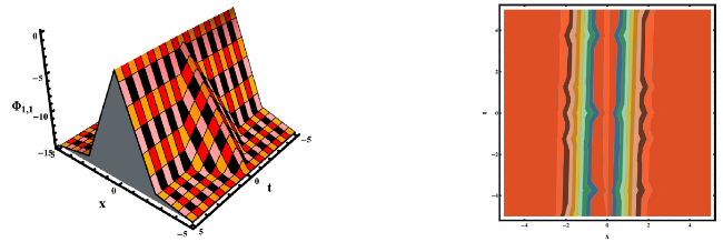
Fig. 1. The graphs of solution (7) for the parameters $\alpha=0.8, \beta=0.02, c=0.03, \zeta_{0}=-0.9, \zeta_{2}=0.4, \nu=0.9, y=0.09, z=0.04$ |
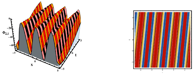
Fig. 2. The graphs of solution (8) for the parameters $\alpha=0.02, \beta=1, c=0.1, \zeta_{0}=-2.4, \zeta_{2}=-2, \nu=0.04, y=0.9, z=0.1$. |
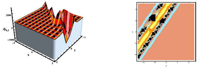
Fig. 3. The graphs of solution (14) for the parameters $\alpha=0.2, \beta=2, c=0.7, \zeta_{0}=0.3, \zeta_{2}=1.7, \nu=2.8, y=1.6, z=1.5$ |
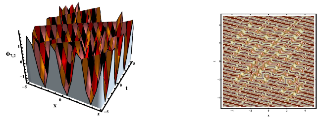
Fig. 4. The graphs of solution (17) for the parameters $\alpha=-1, \beta=0.4, c=-4, \zeta_{0}=-1.3, \zeta_{2}=0.7, \nu=0.7, y=0.4, z=0.2.$ |
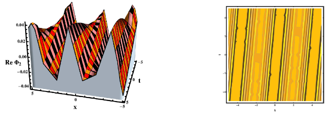
Fig. 5. The graphs of the real behavior of solution $\phi_{2}(x, y, z, t)$ for the parameters $\delta_{2}=0.0025, \delta_{3}=-0.78, \delta_{6}=1, \kappa_{0}=-0.03, \kappa_{1}=0.5, \kappa_{2}=0.07, y=0.7, z=0.1, c=0.09$. |
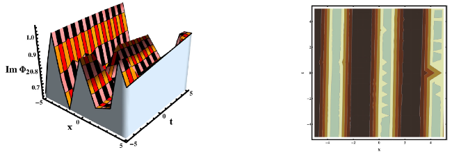
Fig. 6. The graphs of the imaginary behavior of the solution $\left|\phi_{2}(x, y, z, t)\right|$ for the parameters $\delta_{2}=0.5, \delta_{3}=-0.8, \delta_{6}=1.1, \kappa_{0}=0.03, \kappa_{1}=0.3, \kappa_{2}=0.7, y=1, z=0.4, c=0.02$ |

Fig. 7. The graphs of solution $\phi_{2}(x, y, z, t)$ for the parameters $\delta_{2}=1.5, \delta_{3}=0.8, \delta_{6}=2.1, \kappa_{0}=0.3, \kappa_{1}=1.3, \kappa_{2}=0.07, y=1.02, z=0.3, c=0.06$ |
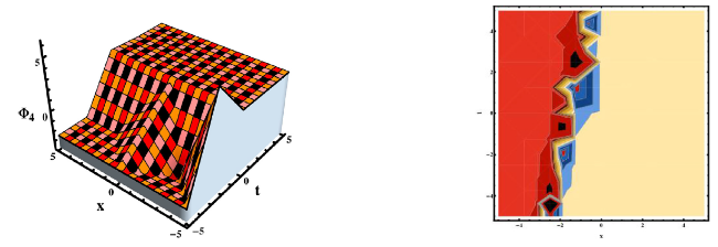
Fig. 8. The graphs of solution $\phi_{4}(x, y, z, t)$ for the parameters $\alpha=0.1, \delta_{2}=2, \delta_{4}=0.2, \kappa_{1}=-0.2, \kappa_{2}=0.7, y=0.09, z=1.7, c=0.198.$ |
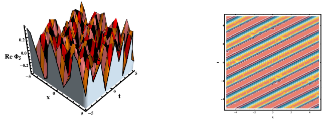
Fig. 9. The plots of real behavior of solution $\Phi_{5}(x, y, z, t)$ with the parameters $\delta_{2}=0.05, \delta_{5}=0.78, \delta_{6}=1, \kappa_{0}=3, \kappa_{0}=0.5, p=0.5, p_{1}=1, y=0.7, z=0.1, c=2$. |
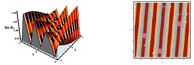
Fig. 10. The plots of imaginary behavior of solution $\Phi_{5}(x, y, z, t)$ for the parameters $\delta_{2}=0.5, \delta_{5}=1.008, \delta_{6}=-0.1, \kappa_{0}=0.3, \kappa_{0}=-0.05, p=1, p_{1}=-1, y=0.05, z=0.01, c=0.087$. |
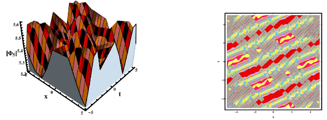
Fig. 11. The plots of solution $\Phi_{5}(x, y, z, t)$ for the parameters $\delta_{2}=1, \delta_{5}=1.8, \delta_{6}=-1.1, \kappa_{0}=2.3, \kappa_{0}=-0.005, p=2, p_{1}=-3, y=0.5, z=0.1 c=1.087$. |
Declaration of Competing Interest
The authors declare that they have no known competing financial interests or personal relationships that could have appeared to influence the work reported in this paper.
Acknowledgments
The authors would like to acknowledge the financial support provided for this research via Open Fund of State Key Laboratory of Power Grid Environmental Protection (No. GYW51202101374) and the National Natural Science Foundation of China (52071298), Zhong Yuan Science and Technology Innovation Leadership Program (214200510010). They also thank the reviewers for their valuable reviews and kind suggestions.
