
1. Introduction
It is well-known that tempered fractional derivatives is in a way a generalization of fractional calculus [1], [2], [3]. Recently, fractional derivatives have been used to describe several phenomena associated with memory and aftereffects due to their non-locality property. Such phenomena are commonplace in physical processes, biological structures, and cosmological phenomena [4], [5], [6]. Several numerical and analytical methods have been presented for this purpose [7], [8], [9]. For instance, the fractional diffusion model of non-Markovian type has been successfully used to characterize the stochastic processes of universal response of mechanical influences and acoustic [10], [11].
Non-linear time-fractional diffusion equations are considered to describe oil pollution in the water. Also, the diffusion equation is widely used in science and engineering as a mathematical model. In particular, tempered fractional derivative which involves fractional term is used in considered many mathematical models. Obtaining the exact solutions of these equations is very important for knowing the wave behavior in ocean engineering models and for the studies related to marine science and engineering. To name few; Marine biology, Biological oceanography and Coastal engineering.
If we multiply the fractional derivatives and integrals by an exponential factor, then this will lead to tempered integrals fractional derivatives [12], [13], [14], [15]. One of the most famous examples is the diffusion equations in terms of tempered fractional derivative, and if we change the standard derivative with respect to space by a tempered derivative, along with the limits of random-walk phenomena govern by distribution of exponential tempered power-law jump [6]. Tempered power-law waiting times lead to tempered fractional time derivatives. It has been proven to be useful for instance in geophysics [6].
The tempered diffusion model has already proven useful in applications to geophysics [6] and finance [16]. In finance, the tempered stable process models price fluctuations with semi-heavy tails, resembling a pure power law at moderate time scales, but converging to a Gaussian at long time scales [17]. Since the anomalous diffusion eventually relaxes into a traditional diffusion profile at late time, this model is also called transient anomalous diffusion. There are many methods that have been implemented to find exact and approximate analytical solutions for TFDEs, such as the fast predictor-corrector approach [7], the fractional spectral method [8], the fractional Jacobi-predictor-corrector algorithm [9], tempered Laplace fractional method [10], the Fractional Reduced Differential Transform Method (FRDTM) [17], [18], fractional natural decomposition method (FNDM) [19], [20], modified extended tanh-function method (METF) [21], fractional Adomian decomposition method (FADM) [22], time differencing methods for multi-dimensional [23] and Time Differencing Schemes [24].
We employed an efficient tool called the tempered fractional natural transform method (TFNTM) to find approximate analytical and exact solutions to tempered fractional linear partial differential equations [25]. This is a new integral transform technique. The method is faster and easy to implement. Indeed, all the calculations can be made with simple analytical manipulations. We have presented proofs of some theorems related to the existence and uniqueness along with error estimate for the TFNTM. We have also considered some classic examples of three tempered fractional diffusion problems and demonstrated that the TFNTM provide solutions, which agree with those obtained in the literature. A notable one is the solution to Black-Scholes equation with tempered fractional derivatives. These are outlined in Section 5.
In finance, see [26], the use of LȨvy processes instead of Gaussian distributions has proven to be an excellent tool in capturing some rare or extreme events in the dynamics of stock prices, such as large movement or jumps over small time step. The FMLS, KoBoL and CGMY models, that follow a jump process or a LȨvy process, have gradually become some of the best choices among practitioners and academics. Therefore, the problem of solving these three models has attracted more and more interest. In the current paper, we consider the tempered fractional BS model for European double-knock-out option. An estimate error along with the existence and uniqueness theorems is also considered. Three examples with exact solutions are chosen in order to illustrate the accuracy and efficiency of TFNT method. The numerical results are in a good agreement with the theoretical analysis. These three fractional models also exhibit higher prices than the classical BS model for in-the-money options which implies the fractional models following the LȨvy processes can more correctly capture the characteristics of a jump or large movement than the classical BS model. We believe that the scheme presented in this paper can also be used in other similar fractional models for pricing different options.
To support these theories and methods of solution, we will apply the (TFNTM) to solve the space and time TFDE of the form:
$\begin{array}{l} { }^{c} D_{t}^{\mu, \lambda}(\phi(x, t))+\alpha \phi(x, t)-\phi_{x x a}(x, t) \\ =h(x, t), \quad(x, t) \in(a, b) \times(0, T] \end{array}$
together with I.C: $\phi(x, 0)=\phi_{0}(x)$, where $h,ϕ_0$ are some given smooth functions, and $α≥0$ is the reaction rate constant.
Furthermore, the tempered BSE of the form Zhang et al. [26]:
$\begin{array}{l} b D_{x}^{\mu, \lambda}(\phi(x, t))-\left(k+b \lambda^{\mu}\right) \phi(x, t) \\ \quad+a \phi_{x}(x, t)+\phi_{t}(x, t)=h(x, t), \quad 1<\mu<2 \end{array}$
subject to the conditions:
$\begin{aligned} \phi(0, t) & =\phi_{x}(0, t)=\phi(1, t)=0,(x, t) \in(0,1) \times[0, T), \phi(x, T) \\ & =e^{-\lambda x} x^{2}(1-x) \end{aligned}$
Note that $D_{x}^{\mu, \lambda}$ is the Riemann-Liouville (R-L) tempered fractional derivative of the function $\phi(x, t)$. Also, $b=\frac{-1}{2} \sigma^{\mu} \sec \left(\frac{\mu \pi}{2}\right), a=r-b, k=r$, where σ represents the rapidly change of an underlying asset and r represents the annualized interest rate of risk-free. This is known to be the most popular application in the market of finance. It worth mentioning that the analysis remains unchanged if we choose an interval outside (0,1). We performed the analysis in the spatial interval (0,1) for the following reasons: given the region $\mathbb{R}^{+}$, after appropriate nondimensionalization (rescaling) of the equations, we can always rescale the finite dimensional domain to a dimensionless spatial interval (0,1). This is a standard procedure in applied science and engineering as referenced, for example, in [27], [28].
The outline of our paper will be as follows. First, we introduce some basic notations and preliminaries about tempered fractional derivatives in Section 2. Section 3 will be devoted to properties and N-transform definitions. Followed by Section 4 where we shall provide detailed proofs for the existence and uniqueness of solutions and perform error analysis for the TFNTM. In Section 5, we provide numerical examples to show effectiveness and reliability of our proposed scheme. In addition, we provide numerical results in Section 6 for the tested model applications. Finally, our conclusion of the present paper will be given in Section 7.
2. Background for tempered fractional derivatives
First, we survey some well-known definitions and properties of tempered fractional derivatives. If [a,b] is an interval on $\mathbb{R}$. Consider $L([a,b])$ to be the Lebesgue integrable on [a,b], i.e.,
$L([a, b])=\left\{\psi:\|\psi\|_{L([a, b])}=\int_{a}^{b}|\psi(s)| d s<\infty\right\}$
where ψ is Lebesgue measurable function.
Definition 1
$\begin{aligned} { }_{a} \mathbb{J}_{s}^{\mu, \lambda}(\psi(s)) & =e^{-\lambda s} a \mathbb{J}_{s}^{\mu}\left(e^{\lambda s} \psi(s)\right) \\ & =\frac{1}{\Gamma(\mu)} \int_{a}^{s} e^{-\lambda(s-\zeta)}(s-\zeta)^{\mu-1} \psi(\zeta) d \zeta, s>a \end{aligned}$
where $a. J_{s}^{\mu}$ denotes the R-L fractional integral:
${ }_{a} \mathbb{I}_{s}^{\mu} \psi(s)=\frac{1}{\Gamma(\mu)} \int_{a}^{s}(s-\zeta)^{\mu-1} \psi(\zeta) d \zeta, \mu>0, s>a$
Clearly, the tempered fractional integral in Eq. (2.1) becomes the R-L fractional integral if $λ=0$. In practical models, sometimes the fractional integral Eq. (2.1) is given as ${ }_{a} D_{s}^{-\mu, \lambda}(\psi(s))$.
Definition 2
$\begin{aligned} { }_{a} D_{s}^{\mu, \lambda}(\psi(s)) & =e^{-\lambda s}{ }_{a} D_{s}^{\mu}\left(e^{\lambda s} \psi(s)\right) \\ & =\frac{e^{-\lambda s}}{\Gamma(k-\mu)} \frac{d^{k}}{d s^{k}} \int_{a}^{s} e^{\lambda \zeta} \psi(\zeta)(s-\zeta)^{k-\mu-1} d \zeta, s>a \end{aligned}$
where ${ }_{a} D_{s}^{\mu}(\psi(s))$ denotes the R-L fractional derivative:
$\begin{aligned} { }_{a} D_{s}^{\mu}(\psi(s)) & =\frac{d^{k}}{d s^{k}}\left(a \mathbb{J}_{s}^{k-\mu}(\psi(s))\right) \\ & =\frac{1}{\Gamma(k-\mu)} \frac{d^{k}}{d s^{k}} \int_{a}^{s} \psi(\zeta)(s-\zeta)^{k-\mu-1} d \zeta, s>a \end{aligned}$
Definition 3
$\begin{array}{l} { }_{a}^{c} D_{s}^{\mu, \lambda}(\psi(s))= e^{-\lambda s}{ }_{a}^{c} D_{s}^{\mu}\left(e^{\lambda s} \psi(s)\right) \\ = \frac{e^{-\lambda s}}{\Gamma(k-\mu)} \int_{a}^{s}(s-\zeta)^{k-\mu-1} \frac{d^{k}}{d \zeta^{k}}\left(e^{\lambda \varsigma} \psi(\zeta)\right) d \zeta \\ s>a \end{array}$
where ${ }_{a}^{c} D_{s}^{\mu}(\psi(s))$ denotes the Caputo fractional derivative:
${ }_{a}^{c} D_{s}^{\mu}(\psi(s))=\frac{1}{\Gamma(k-\mu)} \int_{a}^{s}(s-\zeta)^{k-\mu-1} \frac{d^{d^{k}}}{d \zeta^{(}}(\psi(\zeta)) d \zeta, s>a.$
Definition 4
([7]) Other variants of R-L tempered fractional derivatives are given by:
${ }_{a} \mathbb{D}_{s}^{\mu, \lambda}(\psi(s))=\left\{\begin{array}{lc} { }_{a} D_{s}^{\mu, \lambda}(\psi(s))-\lambda^{\mu} \psi(s), & 0<\mu<1 \\ { }_{a} D_{s}^{\mu, \lambda}(\psi(s))-\mu \lambda^{\mu-1} \frac{d(\psi(s))}{d s}-\lambda^{\mu} \psi(s), 1<\mu<2 \end{array}\right.$
Definition 5
([18]) Let $Γ$ represent the Gamma function, which is given by:
$\Gamma(w)=\int_{0}^{\infty} e^{-s} s^{w-1} d s, w>0$
Remark 1
Throughout this paper, we will use $\Gamma(w+1)=w \Gamma(w)$.
Definition 6
([29]) The Two-parameter Mittag-Leffler function is given as:
$E_{\gamma, \eta}(w)=\sum_{m=0}^{\infty} \frac{w^{m}}{\Gamma(\gamma m+\eta)}, \gamma>0, \eta>0, w \in \mathbb{C}$
Definition 7
([30]) The Adomian polynomials $A_n$ are defined in the form:
$F(v)=\sum_{n=0}^{\infty} A_{n}\left(v_{0}, v_{1}, v_{2}, \ldots, v_{n}\right)$
where the $A_n$’s of the nonlinear term $F(v)$ can easily be computed by the following formula:
$A_{n}=\frac{1}{n!} \frac{d^{m}}{d \lambda^{n}}\left[F\left(\sum_{j=0}^{n} \lambda^{j} v_{j}\right)\right]_{\lambda=0}, n=0,1,2, \cdots$
3. The tempered fractional natural transform method
First, we define the natural transform (N-transform) along with the definition of exponential order function. Consider f(t) with $t \in \mathbb{R}$, then the general integral transform is defined by Belgacem and Silambarasan [31]:
$\mathbb{F}[f(t)](s)=\int_{-\infty}^{\infty} K(s, t) f(t) d t$
where $K(s,t)$ represent the kernel of the transform, s is the real (complex) number which is independent of t. Note that when $K(s,t)$ is $e^{-s t}, t J_{n}(s t)$ and $t^{s-1}(s t)$, then Eq. (3.1) gives, respectively, Laplace transform, Hankel transform and Mellin transform. Now, for $f(t), t \in(-\infty, \infty)$ consider the integral transforms defined by:
$\mathbb{F}[f(t)](u)=\int_{-\infty}^{\infty} K(t) f(u t) d t$
and
$\mathbb{F}[f(t)](s, u)=\int_{-\infty}^{\infty} K(s, t) f(u t) d t$
It is worth mentioning when $K(t)=e^{-t}$, Eq. (3.2) gives the integral Sumudu transform, where the parameter $s$ replaced by $u$. Moreover, for any value of $n$ the generalized Laplace and Sumudu transform are respectively defined by:
$\mathscr{L}[f(t)]=F(s)=s^{n} \int_{0}^{\infty} e^{-s^{n+1} t} f\left(s^{n} t\right) d t$
and
$\mathbb{S}[f(t)]=G(u)=u^{n} \int_{0}^{\infty} e^{-u^{n} t} f\left(t u^{n+1}\right) d t$
Definition 8
Let $f(t)$ be a piecewise continuous function on $\mathbb{R}$. For some $M,K,a,b>0$ with $a<b$, define $A=\left\{f(t):|f(t)|<M e^{a t} \chi_{\left(t_{2}, \infty\right)}(t)+K e^{b t} \chi_{\left(-\infty, t_{1}\right)}(t)\right\}.$. So, $|f(t)| \leq M e^{a t}$ for $t⟶∞$ i.e. $t>t_2$ and $|f(t)| \leq K e^{b t}$ for t⟶−∞ i.e. $t<t_1$.
Note that for any $f(t)$ in the class A with $s,u>0$ we have:
$\begin{array}{l} \left|\int_{-\infty}^{\infty} e^{-s t} f(t u) d t\right| \leq M \int_{0}^{\infty} e^{-s t} e^{a|t u|} d t+K \int_{-\infty}^{0} e^{-s t} e^{b|t u|} d t \\ =M \int_{t_{2}}^{\infty} e^{(a u-s) t} d t+K \int_{-\infty}^{t_{1}} e^{(b u-s) t} d t \end{array}$
Which is convergent provided that $au−s<0$ and $bu−s>0$, which implies that $au<s<bu$ i.e. $a<su<b$. Loosely speaking, $f(t) $ is a function of exponential order.
Then, we define the natural transform as:
$\mathbb{N}(f(t))=R(s, u)=\int_{-\infty}^{\infty} e^{-s t} f(u t) d t, s, u>0$
where $\mathbb{N}$ is the N-transform of $f(t)$ and s and u are the N-transform variables. Note that one can writes Eq. (3.6) as:
$\mathbb{N}(f(t))=\mathbb{N}^{+}(f(t))+\mathbb{N}^{-}(f(t))=R^{+}(s, u)+R^{-}(s, u)$
where,
$\mathbb{N}^{+}(f(t))=R^{+}(s, u)=\int_{0}^{\infty} e^{-s t} f(u t) d t, s, u \in(0, \infty)$
Tempered Fractional Natural Transform Properties
Here are some properties of tempered fractional N-transform:
Property 1. $\mathscr{N}^{+}\left[e^{-\lambda t} t^{\mu}\right]=\frac{u^{\mu}}{(r+\lambda u)^{\mu+1}} \Gamma(\mu+1), \mu>-1$.
Property 2. $\mathscr{N}^{-1}\left[\frac{u^{\eta-1}(r+\lambda u)^{\mu-\eta}}{(r+\lambda u)^{\mu}+\alpha u^{\mu}}\right]=e^{-\lambda t} t^{\eta-1} E_{\mu, \eta}\left(-\alpha t^{\mu}\right)$, where $|\alpha|<\left(\frac{r+\lambda u}{u}\right)^{\mu}$, and $\mu, \eta, \lambda>0$.
4. Convergence and uniqueness of the TFNTM
Here we give proofs to the existence and uniqueness theorems and we give the error analysis for the TFNTM following Picard iteration and the Banach fixed point theorem. Note that the authors of this paper proved Theorem (4.1) and Theorem (4.2) (see, [25]).
Theorem 1
If $m \in \mathbb{Z}^{+}$ such that $m-1<\mu<m$ and $G(r, u)$ is the N-transform of $ψ(s)$, then the N-transform of the R-L tempered fractional derivative is
$\begin{aligned} \mathscr{N}^{+} & {\left[{ }_{a} D_{s}^{\mu, \lambda}(\psi(s))\right]=\left(\frac{r+\lambda u}{u}\right)^{\mu} G(r, u) } \\ & -\sum_{k-0}^{m-1} \frac{(r+\lambda u)^{k}}{u^{k+1}}\left(D^{\mu-(k+1)}\left(e^{\lambda s} \psi(s)\right)\right)_{s=0} \end{aligned}$
Theorem 2
If $m \in \mathbb{Z}^{+}$ such that $m−1<μ<m$ and $G(r,u)$ is the N-transform of the function $ψ(s)$, then the N-transform of the Caputo tempered fractional derivative is:
$\begin{aligned} \mathscr{N}^{+} & {\left[{ }_{a}^{c} D_{s}^{\mu, \lambda}(\psi(s))\right]=\left(\frac{r+\lambda u}{u}\right)^{\mu} G(r, u) } \\ & -\sum_{k=0}^{m-1} \frac{(r+\lambda u)^{\mu-(k+1)}}{w^{\mu-k}}\left(D^{k}\left(e^{\lambda s} \psi(s)\right)\right)_{s=0} \end{aligned}$
Convergence Analysis.
We shall perform the convergence analysis on the nonlinear Riemann-Liouville tempered fractional diffusion equation of the form:
$D_{x}^{\mu_{1} \lambda \lambda}(\phi(x, t))+\phi_{x}(x, t)+\phi_{t}(x, t)-f(\phi(x, t))=h(x, t), 1<\mu<2$
together with conditions:
$\begin{array}{l} \phi(a, t)=\phi(b, t)=0, t \in[T] \\ \phi(x, 0)=\phi_{0}(x), \quad x \in[a, b]. \end{array}$
First, we apply Theorem (4.1) to Eq. (4.1) to obtain:
$\begin{aligned} \Phi(x, r, u)= & \left(\frac{u}{r+\lambda u}\right)^{\mu} \sum_{k=0}^{m-1} \frac{(r+\lambda u)^{k}}{u^{k+1}}\left(D^{\mu-(k+1)}\left(e^{\lambda x} \phi(x, t)\right)\right)_{x=0} \\ + & \left(\frac{u}{r+\lambda u}\right)^{\mu} \mathscr{N}^{+}[f(\phi(x, t)) \\ & \left.-\phi_{x}(x, t)-\phi_{t}(x, t)+h(x, t)\right]. \end{aligned}$
Taking the $\mathscr{N}^{-1}$ of Eq. (4.3) one can obtain:
$\begin{aligned} \phi(x, t)= & w(x, t)+\mathscr{N}^{-1}\left[\left(\frac{u}{r+\lambda u}\right)^{\mu} \mathscr{N}^{+}[f(\phi(x, t))\right. \\ & \left.\left.-\phi_{x}(x, t)-\phi_{t}(x, t)\right]\right] \end{aligned}$
where $w(x,t)$ is coming from the source term. Suppose that the solution is:
$\phi(x, t)=\sum_{n=0}^{\infty} \phi_{n}(x, t)$
The nonlinear term $f(ϕ(x,t))$ becomes:
$f(\phi(x, t))=\sum_{n=0}^{\infty} A_{n},$
where the $A_n$’s are the Adomian polynomials. Using Eq. (4.5), we rewrite Eq. (4.4) in the form:
$\begin{aligned} \sum_{n=0}^{\infty} \phi_{n}(x, t)= & w(x, t)+\mathscr{N}^{-1}\left[\left(\frac{u}{r+\lambda u}\right)^{\mu} \mathscr{N}^{+}\right. \\ & {\left.\left[\sum_{n=0}^{\infty} A_{n}-\sum_{n=0}^{\infty} \phi_{n x}(x, t)-\sum_{n=0}^{\infty} \phi_{n t}(x, t)\right]\right] } \end{aligned}$
Note that $w(x,t)$ represents the initial conditions and the non-homogeneous term.
Looking at both sides of Eq. (4.7), one can conclude that:
$\begin{array}{l} \phi_{0}(x, t)=w(x, t) \\ \phi_{n+1}(x, t)=\mathscr{N}^{-1}\left[\left(\frac{u}{r+\lambda v}\right)^{\mu} \mathscr{N}^{+}\left[A_{n}-\phi_{n t}(x, t)-\phi_{n t}(x, t)\right]\right], n \geq 0 \end{array}$
Finally, the solution is given by the infinite series:
$\phi(x, t)=\sum_{n=0}^{\infty} \phi_{n}(x, t)$
Theorem 3
(Uniqueness). Suppose $0<θ<1$ with, $\theta=\frac{\left(C_{1}+C_{2}+C_{3}\right) e^{-\lambda t} t^{\mu-1}}{\Gamma(\mu)}$. Then the nonlinear tempered fractional diffusion equation in Eq. (4.1) has a unique solution.
Proof
Suppose $\mathbf{B}=(C[\Omega],\|\cdot\|)$ is the Banach space of all continuous functions on $\Omega=[T]$, where $\|\cdot\|$ denotes the norm. We define a mapping $F: \mathbf{B} \rightarrow \mathbf{B}$ with:
$\begin{aligned} \phi_{n+1}(x, t)= & w(x, t)+\mathscr{N}^{-1}\left[\left(\frac{u}{r+\lambda u}\right)^{\mu} \mathscr{N}^{+}\right. \\ & {\left.\left[L\left(\phi_{n}(x, t)\right)+N\left(\phi_{n}(x, t)\right)+M\left(\phi_{n}(x, t)\right)\right]\right] } \end{aligned}$
where, $L[\phi(x, t)]=\phi_{x}(x, t), M[\phi(x, t)]=\phi_{t}(x, t)$ and $N[\phi(x, t)]=f(\phi(x, t))$. Suppose that $L,M$ and $N$ are Lipschitz continuous functions with:
$\begin{array}{l} |M(\phi)-M(\widehat{\phi})|<C_{1}|\phi-\widehat{\phi}|,|L(\phi)-L(\widehat{\phi})|<C_{2}|\phi-\widehat{\phi}| \\ |N(\phi)-N(\widehat{\phi})|<C_{3}|\phi-\widehat{\phi}| \end{array}$
where $C_{1}, C_{2}, C_{3}$ are the Lipschitz constants and $\phi, \widehat{\phi}$ are different solutions. Then:
$\begin{array}{l} \|F(\phi)-F(\widehat{\phi})\| \\ =\max _{t \in \Omega}\left|\begin{array}{l} \mathscr{N}^{-1}\left[\left(\frac{u}{r+\lambda u}\right)^{\mu} \mathscr{N}^{+}[L(\phi)+M(\phi)+N(\phi)]\right] \\ -\mathscr{N}^{-1}\left[\left(\frac{u}{r+\lambda u}\right)^{\mu} \mathscr{N}^{+}[L(\widehat{\phi})+M(\widehat{\phi})+N(\widehat{\phi})]\right] \end{array}\right| \\ =\max _{t \in \Omega}\left|\begin{array}{l} \mathscr{N}^{-1}\left[\left(\frac{u}{r+\lambda u}\right)^{\mu} \mathscr{N}^{+}[L(\phi)-L(\widehat{\phi})]\right] \\ +\mathscr{N}^{-1}\left[\left(\frac{u}{r+\lambda u}\right)^{\mu} \mathscr{N}^{+}[M(\phi)-M(\widehat{\phi})]\right] \\ +\mathscr{N}^{-1}\left[\left(\frac{u}{r+\lambda u}\right)^{\mu} \mathscr{N}^{+}[N(\phi)-N(\widehat{\phi})]\right] \end{array}\right| \end{array}$
So,
$\begin{array}{l} \|F(\phi)-F(\widehat{\phi})\| \leq \max _{t \in \Omega}\left[\begin{array}{l} C_{1} \mathscr{N}^{-1}\left[\left(\frac{u}{r+\lambda u}\right)^{\mu} \mathscr{N}^{+}[|\phi-\widehat{\phi}|]\right]+ \\ C_{2} \mathscr{N}^{-1}\left[\left(\frac{u}{r+\lambda u}\right)^{\mu} \mathscr{N}^{+}[|\phi-\widehat{\phi}|]\right]+ \\ \left.C_{3} \mathscr{N}^{-1}\left[\left(\frac{u}{r+\lambda u}\right)^{\mu} \mathscr{N}^{+}[|\phi-\widehat{\phi}|]\right]\right] \end{array}\right] \\ \left.\leq \max _{t \in \Omega}\left(C_{1}+C_{2}+C_{3}\right)\left[\mathscr{N}^{-1}\left[\left(\frac{u}{r+\lambda u}\right)^{\mu} \mathscr{N}^{+}[|\phi-\widehat{\phi}|]\right]\right]\right] \\ \leq\left(C_{1}+C_{2}+C_{3}\right)\left[\mathscr{N}^{-1}\left[\left(\frac{u}{r+\lambda u}\right)^{\mu} \mathscr{N}^{+}[\|\phi(x, t)-\widehat{\phi}(x, t)\|]\right]\right] \\ =\frac{\left(C_{1}+C_{2}+C_{3}\right) e^{-\lambda t} t^{\mu-1}}{\Gamma(\mu)}\|\phi(x, t)-\widehat{\phi}(x, t)\|. \end{array}$
Since $0<θ<1$, we obtain a contraction mapping. Thus, using the Banach fixed point theorem for contraction mapping, there exists a unique solution of Eq. (4.1). The proof of Theorem (4.3) is complete. □
Theorem 4
(Convergence Theorem). The series solution in Eq. (4.9) of Eq. (4.1) using TFNTM converges whenever, $0<θ<1$ and $\left|\phi_{1}\right|<\infty$.
Proof
Suppose $t_m$ is the $m$ th partial sum, say $t_{m}=\sum_{i=0}^{m} \phi_{i}(x, t)$. We need to show that ${t_m}$ is a Cauchy sequence in B. Using the new formulation of the Adomian polynomials as in [30], we get: $N\left(t_{m}\right)=\widehat{A}_{m}+\sum_{j=0}^{m-1} \widehat{A}_{j}$.
Let $t_n$ and $t_m$ be arbitrary partial sums with $m≥n$. Then:
$\begin{array}{l} \left\|t_{m}-t_{n}\right\|=\max _{t \in \Omega}\left|t_{m}-t_{n}\right| \\ =\max _{t \in \Omega}\left|\sum_{i=n+1}^{m} \widehat{\phi}_{\hat{\delta}}(x, t)\right| \\ \leq \max _{t \in \Omega}\left|\begin{array}{l} \mathscr{N}^{-1}\left[\left(\frac{u}{r+\lambda u}\right)^{\mu} \mathscr{N}^{+}\left[\sum_{i=n+1}^{m} L\left(\phi_{i-1}(x, t)\right)\right]\right]+ \\ \mathscr{N}^{-1}\left[\left(\frac{u}{r+\lambda u}\right)^{\mu} \mathscr{N}^{\prime}+\left[\sum_{i-n+1}^{m} M\left(\phi_{i-1}(x, t)\right)\right]\right]+ \\ \mathscr{N}^{-1}\left[\left(\frac{u}{r+\lambda u}\right)^{\mu} \mathscr{N}^{\mu}+\left[\sum_{i-n+1}^{m} A_{i-1}(x, t)\right]\right] \end{array}\right| \\ =\max _{t \in \Omega}\left|\begin{array}{l} \mathscr{N}^{-1}\left[\left(\frac{u}{r+\lambda u}\right)^{\mu} \mathscr{N}^{\prime}+\left[\sum_{i=n}^{m-1} L\left(\phi_{i}(x, t)\right)\right]\right]+ \\ \mathscr{N}^{-1}\left[\left(\frac{u}{r+\lambda u}\right)^{\mu} \mathscr{N}^{\mu}+\left[\sum_{i=n}^{m-1} M\left(\phi_{i}(x, t)\right)\right]\right]+ \\ \mathscr{N}^{-1}\left[\left(\frac{u}{r+\lambda u}\right)^{\mu} \mathscr{N}^{\mu}+\left[\sum_{i=n}^{m-1} A_{i}(x, t)\right]\right] \end{array}\right|. \end{array}$
Thus,
$\begin{aligned} \left\|t_{m}-t_{n}\right\| & \leq \max _{t \in \Omega}\left|\begin{array}{l} \mathscr{N}^{-1}\left[\left(\frac{u}{r+\lambda u}\right)^{\mu} \mathscr{N}^{+}\left[L\left(t_{m-1}\right)-L\left(t_{n-1}\right)\right]\right] \\ +\mathscr{N}^{-1}\left[\left(\frac{u}{r+\lambda u}\right)^{\mu} \mathscr{N}^{+}\left[M\left(t_{m-1}\right)-M\left(t_{n-1}\right)\right]\right] \\ +\mathscr{N}^{-1}\left[\left(\frac{u}{r+\lambda u}\right)^{\mu} \mathscr{N}^{+}\left[N\left(t_{m-1}\right)-N\left(t_{n-1}\right)\right]\right] \end{array}\right| \\ & \leq \max _{t \in \Omega}\left[\begin{array}{l} \left.C_{1} \mathscr{N}^{-1}\left[\left(\frac{u}{r+\lambda u}\right)^{\mu} \mathscr{N}^{+}\left[\left|t_{m-1}-t_{n-1}\right|\right]\right]+\right] \\ C_{2} \mathscr{N}^{-1}\left[\left(\frac{u}{r+\lambda u}\right)^{\mu} \mathscr{N}^{+}\left[\left|t_{m-1}-t_{n-1}\right|\right]\right]+ \\ C_{3} \mathscr{N}^{-1}\left[\left(\frac{u}{r+\lambda u}\right)^{\mu} \mathscr{N}^{+}\left[\left|t_{m-1}-t_{n-1}\right|\right]\right] \end{array}\right] \\ & \leq\left(C_{1}+C_{2}+C_{3}\right)\left[\mathscr{N}^{-1}\left[\left(\frac{u}{r+\lambda u s}\right)^{\mu} \mathscr{N}^{+}\left[\left\|t_{m-1}-t_{n-1}\right\|\right]\right]\right] \\ & =\frac{\left(C_{1}+C_{2}+C_{3}\right) e^{-\lambda t_{t} \iota^{-1}}}{\Gamma(\mu)}\left\|t_{m-1}-t_{n-1}\right\| \end{aligned}$
So, $\left\|t_{n}-t_{n}\right\| \leq \theta\left\|t_{m-1}-t_{n-1}\right\|.$. Choose $m=n+1$, then we have:
$\left\|t_{n+1}-t_{n}\right\| \leq \theta\left\|t_{n}-t_{n-1}\right\| \leq \theta^{2}\left\|t_{n-1}-t_{n-2}\right\| \leq \ldots \leq \theta^{n}\left\|t_{1}-t_{0}\right\|$
Similarly, using the triangle inequality:
$\begin{aligned} \left\|t_{m}-t_{n}\right\| & \leq\left\|t_{n+1}-t_{n}\right\|+\left\|t_{n+2}-t_{n+1}\right\|+\ldots+\left\|t_{m}-t_{m-1}\right\| \\ & \leq\left[\theta^{n}+\theta^{n+1}+\ldots+\theta^{m-1}\right]\left\|t_{1}-t_{0}\right\| \\ & \leq \theta^{n}\left[\frac{1-\theta^{m-n}}{1-\theta}\right]\left\|\phi_{1}\right\|. \end{aligned}$
But, $0<θ<1$, then $1-\theta^{m-n}<1$. Therefore,
$\left\|t_{m}-t_{n}\right\| \leq \frac{\theta^{n}}{1-\theta} \max _{t \in \Omega}\left|\phi_{1}\right|$
Since $ϕ(x,t)$ is bounded, then $|ϕ_1|<∞$. So, as $n→∞$, we have $\left\|t_{m n}-t_{n}\right\| \rightarrow 0$. Thus, the sequence ${tm}$ is a Cauchy in B. Hence, $\phi(x, t)=\sum_{n=0}^{\infty} \phi_{n}(x, t)$ converges. The proof of Theorem (4.4) is complete. □
Theorem 5
(Error Estimate). The maximum absolute truncation error of the series solution in Eq. (4.9) obtained from Eq. (4.1), is approximated to be:
$\max _{t \in \Omega}\left|\phi(x, t)-\sum_{m=0}^{n} \phi_{m}(x, t)\right| \leq \frac{\theta^{n}}{1-\theta} \max _{t \in \Omega}\left|\phi_{1}\right|.$
Proof
From inequality (4.10), in the proof of Theorem (4.4) we have:
$\left\|t_{m}-t_{n}\right\| \leq \frac{\theta^{n}}{1-\theta} \max _{t \in \Omega}\left|\phi_{1}\right|$
So as $m→∞$, we arrive at $t_{m} \rightarrow \phi(x, t)$. Then,
$\left\|\phi(x, t)-t_{n}\right\| \leq \frac{\theta^{n}}{1-\theta} \max _{t \in \Omega}\left|\phi_{1}(x, t)\right|$
Therefore, the maximum absolute truncation error in Ω is:
$\begin{array}{c} \max _{t \in \Omega}\left|\phi(x, t)-\sum_{m=0}^{n} \phi_{m}(x, t)\right| \leq \max _{t \in \Omega} \frac{\theta^{n}}{1-\theta}\left|\phi_{1}(x, t)\right| \\ =\frac{\theta^{n}}{1-\theta}\left\|\phi_{1}(x, t)\right\|. \end{array}$
This completes the proof of Theorem (4.5). □
Theorem 6
If $0<μ<1$ and $λ≥0$, the tempered fractional I.V.P
${ }^{c} D_{x}^{\mu, \lambda} y(x)+\alpha y(x)=\psi(x), \quad 0 \leq x<\infty$
together with initial condition: $y(0)=y_{0}$, has a solution in the form:
$y(x)=y_{0} e^{-\lambda x} E_{\mu, 1}\left(-\alpha x^{\mu}\right)+\int_{0}^{x} \psi(x-\zeta) e^{-\lambda \zeta} \zeta^{\mu-1} E_{\mu, \mu}\left(-\alpha \zeta^{\mu}\right) d \zeta.$
Proof
Let $\mathscr{N}^{+}[y(x)]=Y(r, u)$ and $\mathscr{N}^{+}[\psi(x)]=\Psi(r, u)$. Apply Theorem (4.2) and the N-transform to Eq. (4.11) to get:
$\begin{aligned} \left(\frac{r+\lambda u}{u}\right)^{\mu} Y(r, u)- & \sum_{k=0}^{n-1} \frac{(r+\lambda u)^{\mu-(k+1)}}{u^{\mu-k}}\left(D^{k}\left(e^{\lambda x} y(x)\right)\right)_{x=0} \\ & +\alpha Y(r, u)=\Psi(r, u) \end{aligned}$
Substituting the initial condition into Eq. (4.12) to arrive at:
$\left(\frac{r+\lambda u}{u}\right)^{\mu} Y(r, u)-y_{0} \frac{(r+\lambda v)^{\mu-1}}{w^{*}}+\alpha Y(r, u)=\Psi(r, u).$
Therefore,
$Y(r, u)=\frac{(r+\lambda u)^{\mu-1} y_{0}}{(r+\lambda u)^{\mu}+\alpha u \psi^{\mu}}+\frac{\Psi(r, u) u^{\psi}}{(r+\lambda u)^{\mu}+\alpha u^{\psi}}$
Using property 2 and taking the inverse operator of Eq. (4.14) and then recalling the property for convolution of the natural transform of two functions, we get:
$y(x)=y_{0} e^{-\lambda x} E_{\mu, 1}\left(-\alpha x^{\mu}\right)+\int_{0}^{x} \psi(x-\zeta) e^{-\lambda \zeta} \zeta^{\mu-1} E_{\mu, \mu}\left(-\alpha \zeta^{\mu}\right) d \zeta.$
This completes the proof of Theorem (4.6). □
5. Applications of TFNT method
To show the reliability and accuracy of our (TFNT) method for solving tempered FDEs, two tempered fractional diffusion equations are discussed, together with the tempered fractional Black-Scholes equation [26]. We present exact solutions to illustrate the efficiency and accuracy of the TFNTM.
Methodology for the Implementation of the TFNT Method
(i) Consider the general linear tempered fractional (PDE) given as:
${ }^{c} D_{t}^{\mu, \lambda} \phi(x, t)+L \phi(x, t)=g(x, t), 0<\mu<1$
together with:
$\phi(x, 0)=h(x)$
where $D_{t}^{\mu, \lambda} \phi(x, t)$ is the Caputo tempered fractional derivative of $ϕ(x,t)$. Here, L represents the linear differential operator and $g(x,t)$ is the non-homogeneous term.
(ii) Employ Theorem (4.2) to Eqs. (5.1) and (5.2) to get:
$\begin{array}{l} \Phi(x, r, u)=\left(\frac{u}{r+\lambda u}\right)^{\mu} \sum_{k=0}^{n-1} \frac{u^{k-\mu}}{(r+\lambda u)^{(k+1)-\mu}} D^{k}\left(e^{\lambda t} \phi(x, t)\right)_{t=0} \\ +\left(\frac{u}{r+\lambda u}\right)^{\mu}\left(\mathscr{N}^{+}[g(x, t)-L \phi(x, t)]\right) \end{array}$
.(iii) Substitute Eq. (5.2) into Eq. (5.3) to arrive at:
$\Phi(x, r, u)=\frac{h(x)}{r+\lambda u}+\left(\frac{u}{r+\lambda u}\right)^{\mu}\left(\mathscr{N}^{+}[g(x, t)-L \phi(x, t)]\right) \text {. }$
(iv) Take $\mathscr{N}^{-1}$-transform of Eq. (5.4) to arrive at:
$\phi(x, t)=\psi(x, t)-\mathscr{N}^{-1}\left[\left(\frac{u}{r+\lambda u}\right)^{\mu}\left(\mathcal{N}^{+}[L \phi(x, t)]\right)\right].$
(v) Assume a solution for $ϕ(x,t)$ of the form:
$\phi(x, t)=\sum_{n=0}^{\infty} \phi_{n}(x, t)$
(vi) Substitute Eq. (5.6) into Eq. (5.5) to get:
$\sum_{n=0}^{\infty} \phi_{n}(x, t)=\psi(x, t)-\mathscr{N}^{-1}\left[\left(\frac{u}{r+\lambda u}\right)^{\mu} \mathscr{N}^{+}\left[L \sum_{n=0}^{\infty} \phi_{n}(x, t)\right]\right].$
Note that $ψ(x,t)$ represents the non-homogeneous term and the initial condition.
(vii) By looking at the two-sides of Eq. (5.7), one obtain:
$\phi_{0}(x, t)=\psi(x, t)$.
(viii) For $n=0$, one gets:
$\phi_{1}(x, t)=-\mathscr{N}^{-1}\left[\left(\frac{u}{r+\lambda u}\right)^{\mu} \mathscr{N}^{+}\left[L \phi_{0}(x, t)\right]\right].$.
(ix) For $n=1$, we have:
$\phi_{2}(x, t)=-\mathscr{N}^{-1}\left[\left(\frac{u}{r+\lambda u}\right)^{\mu} \mathscr{N}^{+}\left[L \phi_{1}(x, t)\right]\right].$.
(x) Finally, in general,
$\phi_{n+1}(x, t)=-\mathscr{N}^{-1}\left[\left(\frac{u}{r+\lambda u}\right)^{\mu} \mathscr{N}^{+}\left[L \phi_{n}(x, t)\right]\right], n \geq 0$
(xi) Hence, our intended solution i.e. Eq. (5.6) is:
$\phi(x, t)=\sum_{n=0}^{\infty} \phi_{n}(x, t)$
Numerical Implementation
Now we apply the proposed methodology to find exact solutions for two tempered diffusion fractional differential equations and tempered fractional Black-Scholes equation.
Example 5.1 [8] Consider the Caputo tempered fractional diffusion equation on Ω=[0,3] with α=0 in Eq. (1.1)
$\begin{aligned} { }^{c} D_{t}^{i, \lambda}(\phi(x, t))- & \phi_{x x x}(x, t)=\frac{2 e^{-\lambda t} t^{2}-\mu}{\Gamma(3-\mu)} \sin (2 \pi x) \\ & +4 \pi^{2} e^{-\lambda t} t^{2} \sin (2 \pi x), 0<\mu<1 \end{aligned}$
together with initial condition:
$\phi(x, 0)=0$
Solution. Employ Theorem (4.2) and Property 1 to Eq. (5.9) to obtain:
$\left(\frac{r+\lambda u}{u}\right)^{\mu} \Phi(x, r, u)-\mathscr{N}^{+}\left[\phi_{x x z}(x, t)\right]=\frac{2 \sin (2 \pi x) u^{2+\mu}}{(r+\lambda u)^{3-\mu}}+\frac{8 \pi^{2} \sin (2 \pi x) u^{2}}{(r+\lambda u)^{3}}.$
Substituting the initial condition from Eq. (5.10) into Eq. (5.11) to get:
$\begin{aligned} \Phi(x, r, u)= & \frac{2 \sin (2 \pi x) u^{2}}{(r+\lambda u)^{3}}+\frac{8 \pi^{2} \sin (2 \pi x) u^{2+\mu}}{(r+\lambda u)^{3+\mu}} \\ & +\left(\frac{u}{r+\lambda u}\right)^{\mu} \mathscr{N}^{+}\left[\phi_{x x}(x, t)\right] \end{aligned}$
Then, apply $\mathscr{N}^{-1}$-transform to both sides of Eq. (5.12) to conclude:
$\begin{aligned} \phi(x, t)= & \mathrm{e}^{-\lambda t} t^{2} \sin (2 \pi x)+\frac{8 \mathrm{e}^{-\lambda t} \pi^{2} t^{2+\mu} \sin (2 \pi x)}{\Gamma(\mu+3)} \\ & +\mathscr{N}^{-1}\left[\left(\frac{u}{r+\lambda u}\right)^{\mu} \mathscr{N}^{+}\left[\phi_{x x}(x, t)\right]\right] \end{aligned}$
Suppose the series solution $ϕ(x,t)$ is of the form:
$\phi(x, t)=\sum_{n=0}^{\infty} \phi_{n}(x, t)$
Combine Eq. (5.14) and Eq. (5.13) to obtain:
$\begin{aligned} \sum_{n-0}^{\infty} \phi_{n}(x, t)= & \mathrm{e}^{-\lambda t} t^{2} \sin (2 \pi x)+\frac{8 \pi^{2} \mathrm{e}^{-\lambda t} t^{2+\mu} \sin (2 \pi x)}{\Gamma(\mu+3)} \\ & +\mathscr{N}^{-1}\left[\left(\frac{u}{r+\lambda u}\right)^{\mu} \mathscr{N}^{+}\left[\sum_{n=0}^{\infty} \phi_{n a x x}(x, t)\right]\right] \end{aligned}$
Looking at both sides of Eq. (5.15), we conclude:
$\begin{array}{l} \phi_{0}(x, t)=\mathrm{e}^{-\lambda t} t^{2} \sin (2 \pi x)+\frac{8 \pi^{2} \mathrm{e}^{-\lambda t} t^{2+\mu} \sin (2 \pi x)}{\Gamma(\mu+3)} \\ \phi_{1}(x, t)=\mathscr{N}^{-1}\left[\left(\frac{u}{r+\lambda u}\right)^{\mu} \mathscr{N}^{+}\left[\phi_{0 x x}(x, t)\right]\right] \\ \phi_{2}(x, t)=\mathscr{N}^{-1}\left[\left(\frac{u}{r+\lambda u}\right)^{\mu} \mathscr{N}^{+}\left[\phi_{1 x x}(x, t)\right]\right] \end{array}$
We proceed in the same manner to get:
$\phi_{n+1}(x, t)=\mathscr{N}^{-1}\left[\left(\frac{u}{r+\lambda u}\right)^{\mu} \mathscr{N}^{+}\left[\phi_{n t e x}(x, t)\right]\right], n \geq 0$
Then using Eq. (5.16) one can calculate the remaining components:
$\begin{aligned} \phi_{1}(x, t)= & \mathscr{N}^{-1}\left[\left(\frac{u}{r+\lambda u}\right)^{\mu} \mathscr{N}^{+}\left[\phi_{0 x x}(x, t)\right]\right] \\ = & \mathscr{N}^{-1}\left[( \frac { u } { r + \lambda u } ) ^ { \mu } \mathscr { N } ^ { + } \left[4 \pi^{2} \mathrm{e}^{-\lambda t} t^{2} \sin (2 \pi x)\right.\right. \\ & \left.\left.-\frac{32 \pi^{4} \mathrm{e}^{-\lambda t} t^{2+\mu} \sin (2 \pi x)}{\Gamma(\mu+3)}\right]\right] \\ = & \frac{-8 \pi^{2} \mathrm{e}^{-\lambda t} t^{2+\mu} \sin (2 \pi x)}{\Gamma(\mu+3)}-\frac{32 \pi^{4} \mathrm{e}^{-\lambda t} t^{2+2 \mu} \sin (2 \pi x)}{\Gamma(2 \mu+3)} \end{aligned}$
Similarly,
$\begin{aligned} \phi_{2}(x, t)= & \frac{-128 \pi^{8} \sin (2 \pi x) e^{-\lambda} t^{2+3 \mu}\left(4 \pi^{2} t^{\mu} \Gamma(2 \mu+3)+\Gamma(3 \mu+3)\right)}{\Gamma(3 \mu+3) \Gamma(2 \mu+3)} \\ \phi_{3}(x, t)= & \frac{-128 \pi^{6} \mathrm{e}^{-\lambda t} t^{2+3 \mu} \sin (2 \pi x)}{\Gamma(3 \mu+3)} \\ & -\frac{512 \pi^{8} \mathrm{e}^{-\lambda t} t^{2+4 \mu} \sin (2 \pi x)}{\Gamma(4 \mu+3)} \end{aligned}$
So, one can compute the other iterations to arrive at the exact solution:
$\begin{aligned} \phi(x, t)= & \phi_{0}(x, t)+\phi_{1}(x, t)+\phi_{2}(x, t)+\ldots \\ = & \mathrm{e}^{-\lambda t} t^{2} \sin (2 \pi x)+\frac{8 \pi^{2} \mathrm{e}^{-\lambda t} t^{2+\alpha} \sin (2 \pi x)}{\Gamma(\mu+3)} \\ & -\frac{8 \pi^{2} \mathrm{e}^{-\lambda t} t^{2+\mu} \sin (2 \pi x)}{\Gamma(\mu+3)} \\ & -\frac{32 \pi^{4} \mathrm{e}^{-\lambda t} t^{2+2 \mu} \sin (2 \pi x)}{\Gamma(2 \mu+3)}+\frac{32 \pi^{4} \sin (2 \pi x) \mathrm{e}^{-\lambda t} t^{2+2 \mu}}{\Gamma(2 \mu+3)} \\ & +\frac{128 \pi^{6} \mathrm{e}^{-\lambda t} \sin (2 \pi x) t^{2+3 \mu}}{\Gamma(3 \mu+3)} \\ & -\frac{128 \pi^{6} \mathrm{e}^{-\lambda t} t^{2+3 \mu} \sin (2 \pi x)}{\Gamma(3 \mu+3)} \\ & -\frac{512 \pi^{8} \mathrm{e}^{-\lambda t} t^{2+4 \mu} \sin (2 \pi x)}{\Gamma(4 \mu+3)}+\ldots \end{aligned}$
in which case the exact solution for Eq. (5.9) will be given by:
$\phi(x, t)=e^{-\lambda t} t^{2} \sin (2 \pi x)$
The exact solution is consistent with the one giving by the local discontinuous Galerkin method in [8].
Observation. Fig. 1 shows that the solution peak is high and one notices that the solutions peak for the tempered diffusion equation as the exponential factor λ increases, will become more smoother.
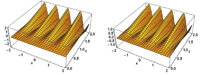
Fig. 1. Solutions for example 5.1 with λ=0.25 and λ=0.6, respectively.. |
Example 5.2 [32] Consider the Riemann-Liouville tempered space-fractional diffusion equation given as:
$\begin{aligned} { }_{0} D_{x}^{\mu, \lambda \lambda}(\phi(x, t))- & \phi_{t}(x, t)=\frac{\Gamma(3+\mu)}{2} e^{-\lambda x} x^{2} t^{2} \\ & -2 t e^{-\lambda x x} x^{2+j \omega}, 0<\mu<1 \end{aligned}$
together with both initial and boundary conditions
$\phi(x, 0)=0, \phi(0, t)=0, \phi(1, t)=e^{-\lambda} t^{2}$
Solution. Apply Theorem (4.1) and Property 1 to Eq. (5.17) to arrive at:
$\begin{aligned} \left(\frac{r+\lambda u}{u}\right)^{\mu} \Phi(x, r, u)- & \sum_{k=0}^{n-1} \frac{(r+\lambda u)^{k}}{u^{k+1}}\left(D^{\mu-(k+1)}\left(e^{\lambda x} \phi(x, t)\right)\right)_{x=0} \\ & -\mathscr{N}^{+}\left[\phi_{t}(x, t)\right]=\frac{\Gamma(3+\mu) u^{2} t^{2}}{(r+\lambda u)^{3}} \\ & -\frac{u^{2+\mu} \Gamma(3+\mu) 2 t}{(r+\lambda u)^{3+\mu}} \end{aligned}$
Substituting the initial conditions into Eq. (5.19) one can arrive easily at:
$\begin{aligned} \left(\frac{r+\lambda u}{u}\right)^{\mu} \Phi(x, r, u)= & \frac{\Gamma(3+\mu) u^{2} t^{2}}{(r+\lambda u)^{3}}-\frac{\Gamma(3+\mu) u^{2+\mu} 2 t}{(r+\lambda u)^{3+\mu}} \\ & +\mathscr{N}^{+}\left[\phi_{t}(x, t)\right] \end{aligned}$
Then,
$\begin{aligned} \Phi(x, r, u)= & \frac{\Gamma(3+\mu) t^{2} u^{2+\mu}}{(r+\lambda u)^{3+\mu}}-\frac{\Gamma(3+\mu) 2 t u^{2+2 \mu}}{(r+\lambda u)^{3+2 \mu}} \\ & +\left(\frac{u}{r+\lambda u}\right)^{\mu} \mathscr{N}^{+}\left[\phi_{t}(x, t)\right] \end{aligned}$
Applying the inverse operator to both sides of Eq. (5.20) one can conclude:
$\begin{aligned} \phi(x, t)= & e^{-\lambda x} x^{2+\mu} t^{2}-\frac{\Gamma(3+\mu)}{\Gamma(3+2 \mu)} 2 t e^{-\lambda x} x^{2 \mu+2} \\ & +\mathscr{N}^{-1}\left[\left(\frac{u}{r+\lambda u}\right)^{\mu} \mathscr{N}^{+}\left[\phi_{t}(x, t)\right]\right] \end{aligned}$
Suppose that the solution $ϕ(x,t)$ is of the form:
$\phi(x, t)=\sum_{n=0}^{\infty} \phi_{n}(x, t)$
Combine Eq. (5.22) and Eq. (5.21) to get:
$\begin{aligned} \sum_{n=0}^{\infty} \phi_{n}(x, t)= & e^{-\lambda z} x^{2+\mu} t^{2}-\frac{\Gamma(3+\mu) 2 t e^{-\lambda x} x^{2 \mu+2}}{\Gamma(3+2 \mu)} \\ & +\mathscr{N}^{-1}\left[\left(\frac{u}{r+\lambda u}\right)^{\mu} \mathscr{N}^{+}\left[\sum_{n=0}^{\infty} \phi_{n t}(x, t)\right]\right] \end{aligned}$
Looking at both sides of Eq. (5.23), one can conclude:
$\begin{array}{l} \phi_{0}(x, t)=e^{-\lambda x} x^{2+\mu} t^{2}-\frac{\Gamma(3+\mu) 2 t e^{-\lambda x} x^{2 \mu+2}}{\Gamma(3+2 \mu)} \\ \phi_{1}(x, t)=\mathscr{N}^{-1}\left[\left(\frac{u}{r+\lambda u}\right)^{\mu} \mathscr{N}^{+}\left[\phi_{0 t}(x, t)\right]\right] \\ \phi_{2}(x, t)=\mathscr{N}^{-1}\left[\left(\frac{u}{r+\lambda u}\right)^{\mu} \mathscr{N}^{+}\left[\phi_{1 t}(x, t)\right]\right] \end{array}$
Thus, we continue to arrive at:
$\phi_{n+1}(x, t)=\mathscr{N}^{-1}\left[\left(\frac{u}{r+\lambda u}\right)^{\mu} \mathscr{N}^{+}\left[\phi_{n t}(x, t)\right]\right], n \geq 0$
Using Eq. (5.24), one can calculate the remaining terms as:
$\begin{aligned} \phi_{1}(x, t)= & \mathscr{N}^{-1}\left[\left(\frac{u}{r+\lambda u}\right)^{\mu} \mathscr{N}^{+}\left[\phi_{0 t}(x, t)\right]\right] \\ = & \mathscr{N}^{-1}\left[\left(\frac{u}{r+\lambda u}\right)^{\mu}\right. \\ & \left.\mathscr{N}^{+}\left[2 t e^{-\lambda x} x^{2+\mu}-\frac{2 \Gamma(3+\mu) e^{-\lambda x} x^{2 \mu+2}}{\Gamma(3+2 \mu)}\right]\right] \\ = & \frac{2 t \Gamma(3+\mu)}{\Gamma(3+2 \mu)} e^{-\lambda x} x^{2+2 \mu}-\frac{2 \Gamma(3+\mu)}{\Gamma(3+3 \mu)} e^{-\lambda x} x^{2+3 \mu} \end{aligned}$
Similarly,
$\phi_{2}(x, t)=\mathscr{N}^{-1}\left[\left(\frac{u}{r+\lambda u}\right)^{\mu} \mathscr{N}^{+}\left[\phi_{1 t}(x, t)\right]\right]=\frac{2 \Gamma(3+\mu)}{\Gamma(3+3 \mu)} e^{-\lambda x} x^{2+3 \mu}$
So, we can compute the other iterations to find the exact solution given as:
$\begin{aligned} \phi(x, t)= & \phi_{0}(x, t)+\phi_{1}(x, t)+\phi_{2}(x, t)+\ldots \\ = & e^{-\lambda x} x^{2+\mu} t^{2}-\frac{\Gamma(3+\mu) 2 t e^{-\lambda x} x^{2 \mu+2}}{\Gamma(3+2 \mu)} \\ & +\frac{2 t \Gamma(3+\mu)}{\Gamma(3+2 \mu)} e^{-\lambda x} x^{2+2 \mu} \\ & -\frac{2 \Gamma(3+\mu)}{\Gamma(3+3 \mu)} e^{-\lambda x} x^{2+3 \mu}+\frac{2 \Gamma(3+\mu)}{\Gamma(3+3 \mu)} e^{-\lambda x} x^{2+3 \mu}+\ldots \end{aligned}$
in which case the exact solution for Eq. (5.17) will be given by:
$\phi(x, t)=e^{-\lambda x} x^{2+\mu} t^{2}$
$\begin{array}{l} b D_{x}^{\mu, \lambda}(\phi(x, t))-\left(k+b \lambda^{\mu}\right) \phi(x, t)+a \phi_{x}(x, t)+\phi_{t}(x, t) \\ \quad=h(x, t), \quad 1<\mu<2 \end{array}$
subject to the conditions:
$\begin{aligned} \phi(0, t) & =\phi_{x}(0, t)=\phi(1, t)=0,(x, t) \in(0,1) \times[0, T), \phi(x, T) \\ & =e^{-\lambda x} x^{2}(1-x) \end{aligned}$
In this model the non-homogeneous part is:
$\begin{aligned} h(x, t)=e^{-\lambda x+(T-t)} & {\left[C x^{2}(1-x)+a\left(2 x-3 x^{2}\right)\right.} \\ & \left.+\frac{\Gamma(3)}{\Gamma(3-\mu)} x^{2-\mu}-\frac{\Gamma(4)}{\Gamma(4-\mu)} x^{3-\mu}\right] \end{aligned}$
where $C=\left(-1-a \lambda-b \lambda^{\mu}-k\right)$.
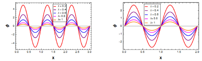
Fig. 2. Solutions for example 5.1 with t=2,3 and different values of λ, respectively. |
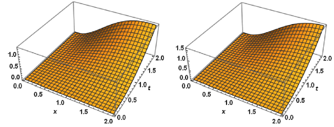
Fig. 3. Solutions for example 5.2 with λ=1.5 and μ=0.75 and μ=1, respectively. |
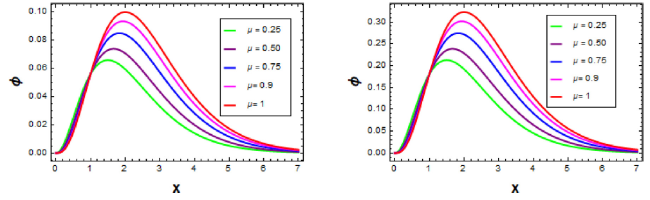
Fig. 4. Solutions for example 5.2 with λ=1.5 and t=0.5 and t=0.9, respectively. |
Solution. Applying Theorem (4.1) to Eqs. (5.25) and (5.26) we obtain:
$\begin{aligned} \Phi(x, r, u)= & \frac{1}{b}\left(\frac{u}{r+\lambda u}\right)^{\mu} \mathscr{N}^{+}\left[\left(k+b \lambda^{\mu}\right) \phi(x, t)\right. \\ & \left.-a \phi_{x}(x, t)-\phi_{t}(x, t)+h(x, t)\right] \end{aligned}$
Note that,
$\begin{aligned} \frac{\left(\frac{u}{r+\lambda u}\right)^{\mu} \mathscr{N}^{+}(h(x, t))}{b}= & \frac{e^{(T-t)}}{b}\left[\frac{2 a u^{\mu+1}}{(r+\lambda u)^{\mu+2}}+\frac{(2 C-6 a) u^{\mu+2}}{(r+\lambda u)^{\mu+3}}\right. \\ & \left.-\frac{6 C u^{\mu+3}}{(r+\lambda u)^{\mu+4}}+\frac{2 u^{2}}{(r+\lambda u)^{3}}-\frac{6 u^{3}}{(r+\lambda u)^{4}}\right] \end{aligned}$
Take the $\mathscr{N}^{-1}$-transform to Eq. (5.27) to get:
$\begin{aligned} \phi(x, t)= & \frac{e^{-\lambda x+(T-t)}}{b}\left[\frac{2 a x^{\mu+1}}{\Gamma(\mu+2)}+\frac{(2 C-6 a) x^{\mu+2}}{\Gamma(\mu+3)}\right. \\ & \left.-\frac{6 C x^{\mu+3}}{\Gamma(\mu+4)}+x^{2}-x^{3}\right] \\ & +\frac{1}{b} \mathscr{N}^{-1}\left[( \frac { u } { r + \lambda u } ) ^ { \mu } \mathscr { N } ^ { + } \left[\left(k+b \lambda^{\mu}\right) \phi(x, t)\right.\right. \\ & \left.\left.-a \phi_{x}(x, t)-\phi_{t}(x, t)\right]\right]. \end{aligned}$
Suppose that the solution $ϕ(x,t)$ is of the form:
$\phi(x, t)=\sum_{n=0}^{\infty} \phi_{n}(x, t)$
Combining Eq. (5.29) and Eq. (5.28), we come up with:
$\begin{aligned} \sum_{n=0}^{\infty} \phi_{n}(x, t)= & \frac{e^{-\lambda x+(T-t)}}{b}\left[\frac{2 a x^{\mu+1}}{\Gamma(\mu+2)}+\frac{(2 C-6 a) x^{\mu+2}}{\Gamma(\mu+3)}\right. \\ & \left.-\frac{6 C x^{\mu+3}}{\Gamma(\mu+4)}+x^{2}-x^{3}\right] \\ & +\frac{1}{b} \mathscr{N}^{-1}\left[( \frac { u } { r + \lambda u } ) ^ { \mu } \mathscr { N } ^ { + } \left[\left(k+b \lambda^{\mu}\right) \sum_{n 0}^{\infty} \phi_{n}(x, t)\right.\right. \\ & \left.\left.-a \sum_{n=0}^{\infty} \phi_{n x}(x, t)-\sum_{n=0}^{\infty} \phi_{n t}(x, t)\right]\right] \end{aligned}$
Looking at both sides of Eq. (5.30), one can conclude:
$\begin{aligned} \phi_{0}(x, t)= & \frac{e^{-\lambda x+(T-t)}}{b}\left[\frac{2 a x^{\mu+1}}{\Gamma(\mu+2)}+\frac{(2 C-6 a) x^{\mu+2}}{\Gamma(\mu+3)}\right. \\ & \left.-\frac{6 C x^{\mu+3}}{\Gamma(\mu+4)}+x^{2}-x^{3}\right] \\ \phi_{1}(x, t)= & \frac{1}{b} \mathscr{N}^{-1}\left[( \frac { u } { r + \lambda u } ) ^ { \mu } \mathscr { N } ^ { + } \left[\left(k+b \lambda^{\mu}\right) \phi_{0}(x, t)\right.\right. \\ & \left.\left.-a \phi_{0 x}(x, t)-\phi_{0 t}(x, t)\right]\right]. \\ \phi_{2}(x, t)= & \frac{1}{b} \mathscr{N}^{-1}\left[( \frac { u } { r + \lambda u } ) ^ { \mu } \mathscr { N } ^ { + } \left[\left(k+b \lambda^{\mu}\right) \phi_{1}(x, t)\right.\right. \\ & \left.\left.-a \phi_{1 x}(x, t)-\phi_{1 t}(x, t)\right]\right]. \end{aligned}$
We continue in this manner to arrive at:
$\begin{aligned} \phi_{n+1}(x, t)= & \frac{1}{b} \mathscr{N}^{-1}\left[( \frac { u } { r + \lambda u } ) ^ { \mu } \mathscr { N } ^ { + } \left[\left(k+b \lambda^{\mu}\right) \phi_{n}(x, t)\right.\right. \\ & \left.\left.-a \phi_{n x}(x, t)-\phi_{n t}(x, t)\right]\right], n \geq 0 \end{aligned}$
From Eq. (5.31), one can obtain:
$\begin{aligned} \phi_{1}(x, t)= & \frac{e^{-\lambda x+(T-t)}}{b^{2}}\left[\frac{-2 a x^{\mu+1}}{\Gamma(\mu+2)}-\frac{6 C\left(1+K+b \lambda^{\mu}\right) x^{\mu+3}}{\Gamma(\mu+4)}\right. \\ & +\frac{2\left(3 a+\left(1+K+b \lambda^{\mu}\right)\right) x^{\mu+2}}{\Gamma(\mu+3)} \\ & \left.+\frac{4 a^{2}(\mu+1)(2 \mu+1) x^{\mu+2}}{\Gamma(2 \mu+3)}\right] \\ & +\frac{e^{-\lambda x+(T-t)}}{b^{2}}\left[\frac{6\left(1+K+b \lambda^{\mu}\right) x^{2 \mu+3}}{\Gamma(2 \mu+4)}\right. \\ & -\frac{4 a(\mu+1)\left(3 a-C+1+K+b \lambda^{\mu}\right) x^{2 \mu+1}}{\Gamma(2 \mu+3)} \\ & \left.-\frac{2\left(C+(C-3 a)\left(K+b \lambda^{\mu}\right)\right) x^{2 \mu+2}}{\Gamma(2 \mu+3)}\right] \end{aligned}$
We proceed in a similar manner to get the remaining iterations using Eq. (5.31), and then the approximate solution will converge to:
$\phi(x, t)=x^{2}(1-x) e^{-\lambda x+(T-t)}.$
The exact solution is consistent with the fast bi-conjugate gradient stabilized method in [26].

Fig. 5. Solutions for example 5.3 for T=0.5 and T=1, respectively. |

Fig. 6. Solutions for example 5.3 for t=0.25 and t=1, respectively. |
6. Tables of numerical calculations
Table 1. Numerical values for example 5.1 for distinct λ′s. |
| x | t | λ=0.25 | λ=0.5 | λ=0.75 | λ=0.9 |
|---|---|---|---|---|---|
| 1/8 | 0.2 | 0.02690483 | 0.02508589 | 0.02434449 | 0.02362501 |
| 0.4 | 0.10237067 | 0.08899678 | 0.08381401 | 0.07893306 | |
| 0.6 | 0.21910048 | 0.17759939 | 0.16231363 | 0.14834349 | |
| 0.8 | 0.37051524 | 0.28002939 | 0.24836379 | 0.22027892 | |
| 1/6 | 0.2 | 0.03295156 | 0.03072382 | 0.02981579 | 0.02893461 |
| 0.4 | 0.12537795 | 0.10899835 | 0.10265078 | 0.09667287 | |
| 0.6 | 0.26834219 | 0.21751395 | 0.19879278 | 0.18168293 | |
| 0.8 | 0.45378665 | 0.34296457 | 0.30418228 | 0.26978548 | |
| 1/3 | 0.2 | 0.03295155 | 0.03072382 | 0.02981579 | 0.02893461 |
| 0.4 | 0.12537795 | 0.10899835 | 0.10265078 | 0.09667286 | |
| 0.6 | 0.26834219 | 0.21751395 | 0.19879278 | 0.18168292 | |
| 0.8 | 0.45378664 | 0.34296456 | 0.30418228 | 0.26978548 |
Table 2. Numerical values for example 5.2 for distinct λ′s. |
| x | t | λ=0.2 | λ=0.4 | λ=0.6 | λ=0.8 |
|---|---|---|---|---|---|
| 0.5 | 0.2 | 0.00639816 | 0.00578930 | 0.00523838 | 0.00473988 |
| 0.4 | 0.02559267 | 0.02315720 | 0.02095350 | 0.01895951 | |
| 0.6 | 0.05758350 | 0.05210371 | 0.04714538 | 0.04265891 | |
| 0.8 | 0.10237066 | 0.09262881 | 0.08381401 | 0.07583806 | |
| 1 | 0.2 | 0.03274923 | 0.02681280 | 0.02195246 | 0.01797316 |
| 0.4 | 0.13099692 | 0.10725120 | 0.08780986 | 0.07189263 | |
| 0.6 | 0.29474307 | 0.24131521 | 0.19757219 | 0.16175843 | |
| 0.8 | 0.52398768 | 0.42900483 | 0.35123944 | 0.28757054 | |
| 2 | 0.2 | 0.15167611 | 0.10167154 | 0.06815247 | 0.04568397 |
| 0.4 | 0.60670445 | 0.40668615 | 0.27260988 | 0.18273587 | |
| 0.6 | 1.36508501 | 0.91504385 | 0.61337223 | 0.41115570 | |
| 0.8 | 2.42681779 | 1.62674461 | 1.09043952 | 0.73094347 |
Table 3. Numerical values for example 5.3 for distinct T′s. |
| x | t | T=0 | T=0.25 | T=0.5 | T=0.75 |
|---|---|---|---|---|---|
| 0.25 | 0.2 | 0.0298888 | 0.0383780 | 0.0492783 | 0.0632746 |
| 0.4 | 0.0244709 | 0.0314213 | 0.0403457 | 0.0518049 | |
| 0.6 | 0.0200351 | 0.0257255 | 0.0330323 | 0.0424143 | |
| 0.8 | 0.0164033 | 0.0210623 | 0.0270445 | 0.0347259 | |
| 0.5 | 0.2 | 0.0620732 | 0.0797035 | 0.1023410 | 0.1314090 |
| 0.4 | 0.0508212 | 0.0652557 | 0.0837900 | 0.1075880 | |
| 0.6 | 0.0416089 | 0.0534269 | 0.0686015 | 0.0880860 | |
| 0.8 | 0.0340665 | 0.0437422 | 0.0561661 | 0.0721187 | |
| 0.75 | 0.2 | 0.0543855 | 0.0698323 | 0.0896665 | 0.1151340 |
| 0.4 | 0.0445270 | 0.0571739 | 0.0734127 | 0.0942638 | |
| 0.6 | 0.0364557 | 0.0468100 | 0.0601052 | 0.0771766 | |
| 0.8 | 0.0298474 | 0.0383248 | 0.0492100 | 0.0631869 |
7. Discussion and conclusion
In this paper, we proved the convergence and existence theorems of tempered fractional natural transform method and gave error estimates for the ensuring approximations. Also, we gave exact solutions for two tempered fractional diffusion equations and we successfully obtained exact solution for the tempered space fractional Black-Scholes equation. The present method obviates the computational difficulties encountered in other traditional methods and all the calculations can be made with simple manipulations. Therefore, it might be considered as a nice alternative to existing techniques and has the potential for wide applications. Clearly, the new scheme presented in this work is highly accurate and efficient: it is devoid of techniques such as linearization, discretization and perturbation. Our aim, in the near future, is to study the extended properties and applications of the proposed TFNTM, examine realistic series, which converge very rapidly, and employ it to nonlinear tempered fractional differential equation problems. This might necessitate the use of existing methods for finding approximate solutions to nonlinear fractional differential equation problems, such as the homotopy perturbation method and the Adomian decomposition method. We believe that our methodology is highly efficient and accurate because we tested our methodology (see examples 5.1-5.3) and obtained very good agreement with the theoretical analysis. We believe that the techniques we have presented in this manuscript, together with the three test examples we provided, can be used in other applied areas, such as in system theory. In our future work, we will apply our methodology to fractional system theoretical problems with sinusoidal initial conditions.
Declarations
Funding.NAO was supported in part by graduate teaching assistantship from the University of Vermont. DEB was supported in part bya Fulbright Scholar Fellowship (PS00289132), Carnegie African Diaspora Fellowship (P00214069), and the University of Vermont through a sabbatical leave.
Compliance with ethical standards
Conflicts of interest. The authors declare that they have no conflict of interest concerning the publication of this manuscript.
Availability of data and materials. Data sharing not applicable to this article as no data sets were generated or analyzed during the current study.
Consent to participate participants is aware that they can contact the University of Vermont Ethics Officer if they have any concerns or complaints regarding the way in which the research is or has been conducted.
Declaration of Competing Interest
The authors declare that they have no known competing financial interests or personal relationships that could have appeared to influence the work reported in this paper.
Acknowledgment
The authors are appreciative for anonymous referees for reading the paper and for their recommendations to improve the manuscript.
