
1. Introduction
Ocean wave information is valuable for a variety of tasks, including marine operations, maritime transport, and ocean environment monitoring. The X-band marine radar has been widely used for ocean wave remote sensing tasks due to its ability to image the sea surface with high temporal and spatial resolutions. Naaijen et al. [1] used X-band radar data to estimate wave elevation while combining a wave propagation and vessel response model to predict future vessel motions. Lyzenga et al. [2] employed X-band Doppler radar data to inverse phase-resolved wave field. Nieto-Borge et al. [3] used a wave monitoring system to derive sea state parameters and compared the results with buoy data. Al-Ani et al. [4] successfully applied a short-term deterministic sea wave prediction (DSWP) technique to the field radar data collected at North Atlantic. The radar sea clutter image is generated through the Bragg resonance interaction between the capillary waves and the electromagnetic waves [5]. It is well-known that gravity waves modulate the backscatter signals through tilt modulation, shadowing modulation, and hydrodynamic modulation [6], [7], and therefore the radar image does not measure the surface elevation directly. The traditional spectral analysis method based on the three-dimensional fast Fourier transform is used to extract wave parameters from radar images [8]. By applying 3D-FFT to a radar image sequence, the image spectrum is estimated, which can then be used to estimate wave spectrum and parameters. Various statistical parameters of the ocean environment can be extracted, such as significant wave height and period, wave direction, sea surface current, and wind speeds [8], [9], [10]. Radar images can also be used for bathymetry mapping [11]. As an example of practical applications, the Wave Monitoring System (WaMos) is based on the spectral analysis method [12], [13]. The statistical parameters provide useful information for relative long-term marine tasks and transport, but they cannot offer quantitative wave information in a specific temporal and spatial location [14]. Therefore, sea surface reconstruction is required, and there are many challenges for various short-term activities, such as ship motion prediction, vessel positioning, and helicopter landing [15].
Compared to statistical parameters, reconstructed sea surface elevation can provide more accurate wave height information in both spatial and temporal domains. The standard reconstruction method [7] is based on spectral analysis: using the dispersion relationship to filter the image spectrum and extract the wave-related signals, followed by the modulation transfer function to correct the shadowing modulation effect. The standard reconstruction method has been widely used in various studies for wave [13] and ship motion prediction [16]. However, the filtering process introduces several empirical parameters that need to be calibrated for a given radar system and wave environment. Moreover, to obtain the scaled sea surface elevation maps, significant wave height must be calculated, usually through signal-to-noise ratio. To address these issues, Qi et al. [17] proposed a parameter optimization method using concurrent phased-resolved wave field simulations based on the high-order spectral method [18]. This approach significantly improves the consistency and fidelity of the reconstruction.
Zinchenko et al. [14] introduced another modification to the standard method by transforming the radar image intensity from the non-negative range to a ”wave-elevation”-like representation with a near-zero mean. They also used the parameter optimization method based on the simulated wave field. In addition to the standard method, several alternative methods have been proposed over the years. Greenwood et al. [19] proposed a method to supplement the backscatter with an artificial second-order Stokes wave to fill the missing wave troughs caused by shadowing modulation. Dankert and Rosenthal [6] presented an empirical inversion method based on the determination of the surface tilt angle in the antenna look direction at each pixel of the radar images. This inversion method is useful in areas where the tilt modulation is more dominant and does not require external calibration to scale the wave amplitude. Naaijen and Wijaya [20] provided a beam-wise analysis to translate the image information to wave elevation. The basic idea is to apply the one-dimensional fast Fourier transform (1D-FFT) to each beam in the radar image in polar coordinates and then apply a high-pass filter when conducting the inverse transformation. Unlike the standard method or tilt angle-based method, the beam-wise analysis method can process radar images one by one, and thus a sequence of radar images is not required.
In the last few years, machine learning models have shown great potential to address scientific problems in various areas such as biological [21], human health [22], and e-commerce [23]. As an important branch of deep learning models, convolutional neural networks (CNN) have demonstrated great potential in handling various computer vision tasks [24], [25], [26]. As a result, multiple studies have implemented the CNN model to extract wave parameters from radar images. Duan et al. [27] researched the inversion of significant wave height and peak period from synthetic radar images using Alex-Net [28] and visual geometry group network (VGG-Net) [29]. Compared to the conventional spectral analysis method, the CNN-based models have produced higher accuracy. To extract both spatial and temporal features from radar images, the convolutional gated recurrent unit network (CGRUN) [30] and temporal convolutional network (TCN) [31], [32] are used for significant wave height estimation. In [30], CGRUN fundamentally connects the gated recurrent unit network (GRUN) to the end of the CNN, where the CNN is used for spatial feature extraction and GRUN for temporal feature extraction. In [31], a feature vector extracted from radar images is the direct input to the TCN. The feature vector is acquired by applying signal-to-noise ratio analysis [9], ensemble empirical mode decomposition [33], and gray level cooccurrence matrix methods [34] to radar images. Other machine learning methods, such as support vector machines [35], [36] and artificial neural networks [37], are also utilized for significant wave height estimation.
It has been demonstrated that it is possible to extract phased-averaged wave parameters using the CNN model. Drawing inspiration from this, we have proposed a novel approach to recover sea surface elevation maps from radar images using a CNN-based model. In this task, the inputs are radar images, and the outputs are sea surface elevation maps. This necessitates an image-to-image model for the CNN-based model, and thus, we have employed the U-Net model in this study. U-Net was first introduced in [38] for biomedical image segmentation and has since been developed and used in many other fields [39], [40], [41]. The CNN-based model is an end-to-end system that automatically learns to translate radar images into surface elevation maps. Therefore, it does not require external calibration or empirical parameters. The convolutional and pooling layers are utilized to learn the textural features in radar images and subsequently reconstruct the wave field.
The rest of this paper is organised as follows. Section 2 explains the numerical simulation approach used to produce artificial sea surface and radar images. Section 3 describes the proposed CNN approach and the benchmark method for comparison, which is the spectral analysis reconstruction technique. Section 4 displays the findings and discussion. Finally, Section 5 summarises the conclusions of the study.
2. Numerical simulation of radar images
2.1. Synthetic sea surface elevation maps
The standard linear wave model [42] is employed to generate sea surface elevation maps. The sea surface elevation is created as a linear sum of regular wave components with differing frequencies and directions. In this study, the ITTC (International Towing Tank Conference) two-parameter wave spectrum is selected as the target wave spectrum. This wave spectrum is expressed as:
$S(\omega)=\frac{173 H_{s}^{2}}{T_{p}^{4} \omega^{5}} \exp \left(-\frac{691}{T_{p}^{4} \omega^{4}}\right)$
Here, $H_s$ denotes the significant wave height, while $T_p$ represents the spectral peak period of the wave.
To compute the directional wave spectrum, a propagation direction is assigned to each wave component using a directional spreading function $G(θ)$:
$G(\theta)=\frac{2}{\pi} \cos ^{2}\left(\theta-\theta_{p}\right),\left|\theta-\theta_{p}\right|<\frac{\pi}{2}.$
Here, $θ_p$ denotes the primary direction. Consequently, the directional wave spectrum can be expressed as $S(\omega, \theta)=S(\omega) \cdot G(\theta)$.
Finally, the wave elevation η at spatial coordinate (x,y) and temporal coordinate t is expressed as follows:
$\eta(x, y, t)=\sum_{i=1}^{n} \sum_{j=1}^{m} a_{i j} \cos \left[\omega_{i} t-k_{i}\left(x \cos \theta_{j}+y \sin \theta_{j}\right)+\varepsilon_{i j}\right].$
Here, $ω_i$ is the frequency of the wave, and $k_i$ is the wavenumber, which is calculated using the dispersion relation: $\omega_{i}{ }^{2}=g k_{i}$. The amplitude $a_{i j}=\sqrt{S\left(\omega_{i}, \theta_{j}\right) \Delta \omega \Delta \theta}$ is calculated using the spectral density function $S\left(\omega_{i}, \theta_{j}\right)$, and Δω and Δθ are the frequency and directional bin widths, respectively. The phase $ε_{ij}$ is randomly selected from a uniform distribution between 0 and 2π.
The sea surface is modelled over an area of [−2000m,2000m]2 with a spatial resolution of dx=dy=5m for the x and y axes, and a temporal resolution of dt=1s. For simplicity, Fig. 1(a) shows a snapshot of the synthesised sea surface at a particular time using a specific parameter set. The snapshot has been transformed to polar coordinates (r,θ) on a grid with dr=5m and dθ=0.3∘.
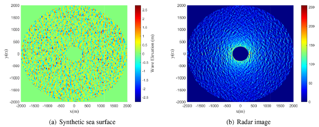
Fig. 1. Snapshot of the synthetic sea surface and the radar image. |
2.2. Shadowing and tilt modulation
The numerical simulation of shadowing and tilt modulation is based on [7]. To format the sea surface elevation map for radar imaging, it needs to be converted to the polar coordinate system. The wave field in polar coordinates is denoted as η(r,θ,t). In a given azimuth, the grazing incidence angle at different ranges is $\alpha(r, t)=\arctan (r /[H-\eta(r, \theta, t)])$, where H represents the height of the radar antenna above sea level. For each beam (where θ is constant), if there is a position where $r_0<r$ and the grazing incidence angle $\alpha_{0}\left(r_{0}, t\right) \geq \alpha(r, t)$, then the signal at coordinate (r,t) will be shadowed. The simulated shadowing modulation is given by
$\sigma_{\mathrm{sh}}(r, \theta, t)=\left\{\begin{array}{ll} \sigma(r, \theta, t) & \text { no shadowing occurs } \\ 0 & \text { otherwise } \end{array}\right.$
where σ(r,θ,t) is the result of scaling η(r,θ,t) into 256 gray levels.
Tilt modulation is caused by the local incidence, which is calculated using the scalar product between the 3D exterior normal vector $\mathbf{n}(r, \theta, t)=\left(-\partial_{r} \eta,-\partial_{\theta} \eta / r, 1\right)$ to the sea surface, and the 3D vector $\mathbf{u}(r, \theta, t)=(-\sin \alpha, 0, \cos \alpha)$. The vector u(r,θ,t) is defined as the vector from the observed position to the radar antenna, where α is the grazing incidence angle as defined above.
The simulated tilt image is given by
$\mathscr{T}(r, \theta, t)=\frac{\mathbf{n}(r, \theta, t) \cdot \mathbf{u}(r, \theta, t)}{|\mathbf{n}||\mathbf{u}|}$
After combining the shadowing and tilt modulation with the sea surface elevation map, the radar signal is given by
$\sigma_{\text {tilt }}(r, \theta, t)=\left\{\begin{array}{ll} \mathscr{T}(r, \theta, t) & \text { if } \mathscr{T}(r, \theta, t)>0 \text { and } \sigma_{\text {shh }}(r, \theta, t) \neq 0 \\ 0 & \text { otherwise. } \end{array}\right.$
Afterwards, the $\sigma_{\text {tilt }}$ values are encoded with 256 gray levels. Finally, white Gaussian noise is added to the synthetic radar image data to simulate the radar system noise. The mean and variance of the white Gaussian noise are 0 and 1, respectively. The radar antenna is assumed to be fixed at a height of 37m. The shadowing and tilt modulation are applied to the synthetic sea surface, with the radar blind area set to be r<300m. An example of the resulting radar image is shown in Fig. 1(b).
3. Reconstruction of sea surface from radar images
3.1. The spectral analysis method
The frequency and wavenumber of gravity waves, denoted by ω and $\mathbf{k}=\left(k_{x}, k_{y}\right)$, respectively, are related by the linear dispersion relationship $\omega^{2}(\mathbf{k})=g|\mathbf{k}|$, where g is the gravitational acceleration. The conventional approach to reconstructing wave fields from radar images involves using the three-dimensional fast Fourier transform to derive the radar image spectrum in the frequency-wavenumber domain and extracting wave-related signals by applying the dispersion relationship. To correct for the influence of shadowing and tilt modulation, a modulation transfer function is used to adjust the wave spectrum. The standard method for wave field reconstruction involves the following five main steps:
(1) To obtain the amplitude and phase spectrum of the radar image, the 3D-FFT method is applied to the radar image sequence, denoted as $A(\mathbf{k}, \omega)$ and $\phi(\mathbf{k}, \omega)$, respectively. The 3D-FFT method requires a sequence of 2N continuous radar images, where $N$ is an integer. In this paper, we selected a sequence of 128 continuous radar images for the 3D-FFT process.
(2) To extract the wave-related components from the radar image spectrum, a high-pass filter $\left(\omega>\omega_{0}\right)$ and a band-pass filter $\left(\omega_{1} \leq \omega \leq \omega_{2}\right)$ are utilized. The high-pass filter is used to reduce low-frequency signals caused by long-range dependence modulation effects, with a cutoff frequency of $\omega_{0}=0.06 \cdot \pi=0.188 \mathrm{rad} / \mathrm{s}$. For the band-pass filter, the cutoff frequencies are usually defined as $\omega_{1,2}(\mathbf{k})=\omega(\mathbf{k}) \pm b \cdot \Delta \omega$, where Δω is the frequency resolution after the 3D-FFT process. Because the radar sequence contains 128 images, the frequency resolution is relatively small, and we set the bandwidth as 8Δω with b=4. The filtered amplitude and phase spectrum are denoted as $\widehat{A}(\mathbf{k}, \omega)$ and $\widehat{\phi}(\mathbf{k}, \omega)$, respectively.
(3) A modulation transfer function (MTF) is utilized to mitigate the shadowing modulation effect, which is more pronounced in the far range of the radar image. The MTF is expressed as $M(k)=k^{-\beta}$, where β is an empirical coefficient dependent on the sea state. In the inversion process described in [7], β=1.2 was used. However, in our research, we observed that a value of β=0.7 yields significantly improved outcomes. Therefore, we apply this coefficient to correct the spectrum, which is expressed as $A_{\tilde{\eta}}(\mathbf{k}, \omega)=\widehat{A}(\mathbf{k}, \omega) \cdot k^{-0.7}$.
(4) To obtain the unscaled sea surface elevation $\tilde{\eta}(x, y, t)$, apply the inverse 3D-FFT to the wave amplitude spectrum $\mid A_{\tilde{\eta}}(\mathbf{k}, \omega)$ and phase spectrum $\widehat{\phi}(\mathbf{k}, \omega)$.
(5) The actual wave elevation η(x,y,t) can be obtained by scaling $\tilde{\eta}(x, y, t)$ using the relationship between the standard deviation of wave elevation ση˜ and the significant wave height $H_s$, given by
$\eta(x, y, t)=c \tilde{\eta}(x, y, t) \text {, }$
where $c=\frac{H_{8}}{4 \sigma_{i j}}$.
3.2. The CNN-based model
The concept of using a convolutional neural network to reconstruct the sea surface from the radar image involves an image-to-image process where the input to the network is the radar image, and the output is the sea surface elevation map. Compared to the spectral analysis method, the CNN-based model is a straightforward end-to-end model. To implement this, we adopted a classical image-to-image network proposed by Ronneberger et al. [38] and made modifications to the layers to match the size of the input and output images.
The U-Net model architecture, as depicted in Fig. 2, follows an image-to-image approach. The input of the network is the radar image, and the output is the sea surface elevation map. The model consists of a contracting path and an expansive path. The contracting path is a convolutional network comprising convolution layers and pooling layers. Each convolution layer is composed of two 3x3 convolutions, batch normalization, and rectified linear unit (ReLU). The feature channels are doubled after each convolution layer. The pooling layer performs a 2x2 max pooling operation with a stride of 2 to downsample. The expansive path involves upsampling of the feature map, followed by a 3x3 convolution that halves the number of feature channels, a concatenation with the corresponding feature map from the contracting path, and two 3x3 convolution operations, each followed by a ReLU. Finally, the output channel is obtained using a 1x1 convolution operation. The U-Net model comprises multi-channel feature maps, and the number of channels is indicated at the top of the blue box. The square’s size is shown at the lower left edge, and copied feature maps are represented by green squares.

Fig. 2. The architecture of the CNN-based model. |
The original radar image is in polar coordinates with varying widths and heights. To use the entire image as input, we convert the radar image to the Cartesian coordinate system with dx=dy=5m. The converted image size is 801x801. We remove the right column and bottom row pixel values to obtain an appropriate input size of 800x800 for the network. The blind area (r<300m) and outside area (r>2000m) are set to 0. To remove the influence of different display formats of radar images, we use the radar image gray level as the input, resulting in a single input channel. The output of the network is the surface elevation map, which contains only the wave height values at each position, resulting in a single output channel. During training, we set the value in the blind and outside areas to 0 in each output image before calculating the loss to remove their influence. Essentially, this is an image-to-image regression problem, and we choose the mean square error (MSE) function as the loss function.
The CNN-based model is trained and tested on a Linux operating system, using an NVIDIA A100 GPU with 80-GB memory.
3.3. Definition of evaluation parameters
In this paper, we selected the correlation coefficient (Corr), non-dimensional root mean square error (NDRMSE), and relative error (RE) as parameters to evaluate the performance of the spectral analysis method and the CNN-based model on wave field reconstruction. The correlation coefficient assesses the fidelity of the wave shape, while the non-dimensional root mean square error indicates the deviation of wave elevation values.
The definition of the correlation coefficient (Corr) is given by
$\text { Corr }=\frac{\sum_{\mathbf{x}}\left(\eta_{\mathrm{r}}(\mathbf{x})-\bar{\eta}_{\mathrm{r}}\right)(\eta(\mathbf{x})-\bar{\eta})}{\sqrt{\sum_{\mathbf{x}}\left(\eta_{\mathrm{r}}(\mathbf{x})-\bar{\eta}_{\mathrm{r}}\right)^{2} \sum_{\mathbf{x}}(\eta(\mathbf{x})-\bar{\eta})^{2}}}$
On the other hand, the non-dimensional root mean square error (NDRMSE) is given by
$\mathrm{NDRMSE}=\sqrt{\frac{\sum_{\mathrm{x}}\left(\eta_{+}(\mathrm{x})-\eta(\mathrm{x})\right)^{2}}{N}} / H_{s}$
Here, $η_r$ represents the reconstructed sea surface, while η represents the actual synthetic sea surface. $\bar{\eta}_{\tau}$ and $\bar{\eta}$ represent the means of the reconstructed sea surface and the actual sea surface, respectively. $N$ is the total number of points used to represent the simulated sea surface area.
The point-to-point relative error (RE) is used to assess the accuracy of wave height reconstruction at individual locations in the radar image. It is defined as:
$\operatorname{RE}(\mathbf{x})=\frac{\left|\eta_{r}(\mathbf{x})-\eta(\mathrm{x})\right|}{H_{y}}$
where $\eta_{r}(\mathbf{x})$ is the reconstructed wave height at position $\mathbf{x}, \eta(\mathbf{x})$ is the actual wave height at that position, and $H_s$ is the significant wave height. The RE provides insight into the reconstruction differences across different areas of the radar image.
4. Results and discussion
4.1. Comparisons of the CNN-based model and spectral analysis method
In order to achieve optimal performance from the CNN-based model, a significant amount of data is required for the training process. As such, we generated 3075 radar images across various sea states for this purpose. To simplify the process of data generation, we utilized the wave steepness parameter, denoted by s, to control the relationship between the significant wave height $H_s$ and the wave peak period $T_p$. This parameter is defined as follows:
$s=\frac{H_{s}}{\lambda_{p}}=\frac{2 \pi H_{3}}{g T_{y}^{2}}$
Here, $\lambda_{p}=2 \pi / k_{p}=2 \pi g / \omega_{p}^{2}=2 \pi g /\left(2 \pi / T_{p}\right)^{2}=g T_{p}^{2} / 2 \pi$ represents the wavelength of the wave component relative to the peak frequency.
For the training data, we selected a value of s=0.04, with $T_p$ ranging from 6s to 10s, and generated 75 images every 0.1s. Using the wave steepness parameter, $H_s$ can be calculated accordingly. The primary propagation direction in the training data is $θ_p=0^∘$. The training dataset was randomly divided into a training and validation set at an 8:2 ratio. The training options for the CNN-based model are outlined in Table 1. The learning rate begins to decrease after the epoch reaches 30, with a decay factor of 1/70.
Table 1. Training options for the CNN-based model. |
| Network | U-Net |
|---|---|
| Solver | Adam[43] |
| Number of epochs | 100 |
| Size of mini-batch | 4 |
| Initial learning rate | 0.0002 |
To compare the effectiveness of the spectral analysis method and the CNN-based model, we generated an additional 1024 radar images using the same wave steepness. To ensure that the sea state parameters did not overlap with those of the training data, we varied the peak period from 6.13s to 9.77s and generated 128 images at intervals of 0.52s. Details regarding the sea state parameters for the test data can be found in Table 2.
Table 2. The sea state parameters for the test dataset with s=0.04. |
| Sequence Number (sea state) | $H_s$(m) | $T_p$(s) |
|---|---|---|
| 1 | 2.344 | 6.13 |
| 2 | 2.759 | 6.65 |
| 3 | 3.207 | 7.17 |
| 4 | 3.689 | 7.69 |
| 5 | 4.205 | 8.21 |
| 6 | 4.755 | 8.73 |
| 7 | 5.338 | 9.25 |
| 8 | 5.955 | 9.77 |
After applying both the conventional method and the CNN-based method, we calculated Corr and NDRMSE for each radar image snapshot. The averaged evaluation parameters across different sea states are presented in Fig. 3, while Table 3 displays the average Corr and NDRMSE values for all 1024 images. To demonstrate the accuracy changes in different ranges, we selected two typical areas, Area1 (300m<r<800m) and Area2 (300m<r<2000m), for visualisation purposes. Area1 corresponds to the near radar area, while Area2 represents the entire radar image. In Fig. 3, the CNN-based model and spectral analysis method are respectively represented by blue lines with circles and red lines with squares. The solid line denotes the value of Area1, while the dashed line denotes the value of Area2.
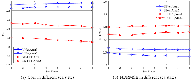
Fig. 3. Comparisons between the CNN-based model and spectral analysis method in various sea states. |
Table 3. The average Corr and NDRMSE values after applying the CNN-based model and the conventional spectral analysis method. |
| Area1 | Area2 | |||
|---|---|---|---|---|
| Corr | NDRMSE | Corr | NDRMSE | |
| 3D-FFT | 0.8701 | 0.1243 | 0.7898 | 0.1515 |
| U-Net | 0.9874 | 0.0390 | 0.9676 | 0.0624 |
The findings indicate that the CNN-based model outperforms the spectral analysis method across various sea states. Specifically, the Corr in Area2 improved from 0.78−0.80 to 0.96−0.97, and the NDRMSE in Area2 decreased from 0.148−0.155 to 0.061−0.067. Additionally, according to the results, rescaling will not have a significant impact on the CNN prediction, as described in detail in Appendix A. The conventional method’s accuracy slightly decreases with an increase in significant wave height due to shadowing modulation, leading to more shadowed areas in the radar image. In contrast, the CNN-based model performs better in higher significant wave height sea states. This indicates that the CNN-based model can learn the wave distribution characteristic from the texture of radar images, enabling it to fill shadowed areas with reasonable wave elevation values. However, as $H_s$ and $T_p$ change in different sea states, this conclusion is based on preliminary observations of experimental results. Thus, we cannot determine whether $T_p$ or $H_s$ has a greater influence on the accuracy.
According to Table, the spectral analysis method achieved Corr values of 0.8701 and 0.7898 in Area1 and Area2, respectively. As shown in Fig. 4, the spectral analysis method had better accuracy in the near radar area, where the effects of shadowing modulation and tilt modulation were relatively weak. This indicates that sufficient wave elevation information remains in the near radar area. However, as the area expands to the outer range, the accuracy drops significantly and the relative error is much higher. On the other hand, the difference in Corr between Area1 and Area2 for the CNN-based model is smaller (0.0198) compared to the spectral analysis method (0.0803), despite the NDRMSE in Area2 still being relatively higher than in Area1. The relative error map shows that the error is higher in the far-range area. Nevertheless, the CNN-based model has obvious advantages over the conventional spectral analysis method.
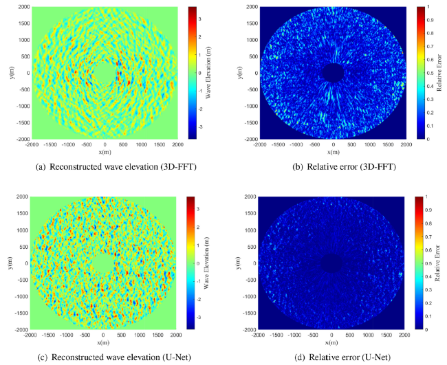
Fig. 4. Comparisons between the outcomes of the spectral analysis method and the CNN-based model. |
4.2. Dependence of CNN-based model on training data
The performance of the CNN-based model is highly dependent on the characteristics of the training data, and it may produce poor results when tested on data with different characteristics. In this section, we assess the generalization ability of the model by testing it on different test data. The main propagation direction of the training data is $\theta_{p}=0^{\circ}$, and the wave steepness is s=0.04. First, we test the model’s performance with and without random rotation using data from various main propagation directions. Random rotation is used to enhance the model’s generalization ability. Next, we test the model’s performance on four sets of data with varying wave steepness to assess its ability to perform outside the coverage of the training data. To improve the accuracy of data beyond the initial training data coverage, we generated two sets of expanded training data for further training of the model.
As mentioned above, the training data has a main propagation direction of $\theta_{p}=0^{\circ}$. However, to cover a wider range of main propagation directions, radar images are randomly rotated before being fed into the network. The rotation angles used are $\left[-90^{\circ},-40^{\circ}, 0^{\circ}, 45^{\circ}, 90^{\circ}\right]$, allowing the CNN-based model to recognize wave patterns in different directions. To test the CNN-based model, eight sets of test data are used, with main propagation directions of $-90^{\circ},-60^{\circ},-45^{\circ},-20^{\circ}, 20^{\circ}, 45^{\circ}, 60^{\circ}, 90^{\circ}$. The corresponding sea state parameters are listed in Table 4, and 20 radar images are generated for each sea state.
Table 4. Sea state parameters of test data for each main propagation direction. |
| Sequence number | $H_s$(m) | $T_p$(s) |
|---|---|---|
| 1 | 3.189 | 7.15 |
| 2 | 3.463 | 7.45 |
| 3 | 3.747 | 7.75 |
| 4 | 4.043 | 8.05 |
| 5 | 4.350 | 8.35 |
| 6 | 4.668 | 8.65 |
| 7 | 4.997 | 8.95 |
The wave steepness of all the data tested previously was 0.04, which is identical to that of the training data. To evaluate the model’s performance under different wave steepness, we selected four additional wave steepness values (s=0.02, s=0.03, s=0.05 and s=0.06) to generate test data. For s=0.02 and s=0.03, $T_p$ ranged from 8.5s to 10s with an interval of 0.1s, whereas for s=0.05 and s=0.06, $T_p$ ranged from 6s to 7.5s with the same interval of 0.1s. The variation in wave peak periods for different wave steepness was to prevent the parameters from exceeding the range of the training data. The $H_s$ value corresponded one-to-one with the $T_p$ value through Eq. 11. Each $T_p$ and $H_s$ pair was regarded as a sea state.
Fig. 5(a) and Fig. 5(b) depict the reconstruction results without and with random rotation, respectively. It is evident that incorporating random rotation in the image can significantly enhance the accuracy in different primary directions. The Corr has improved from 0.77−0.95 to 0.95−0.97. Furthermore, the NDRMSE has decreased from 0.077−0.160 to 0.061−0.076. By including random rotation during the training process, the model can also perform well on data with different wave directions. This method is highly beneficial when the amount of data for training is limited. The results in Fig. 5(b) indicate that the accuracy in ±90∘ and ±20∘ is higher than in other directions. The accuracy is higher for results with the main direction as ±90∘ because the images after random rotation with angles as −90∘ and 90∘ have similar patterns. Similarly, the accuracy is higher for results with the main direction as ±20∘ because they are closer to the main direction of the training data. Overall, the CNN-based model’s accuracy in different primary directions is satisfactory, which implies that we do not require more data to train the model, but only need to add random rotation to the training process.
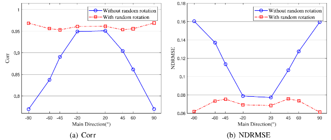
Fig. 5. The Corr and NDRMSE of all the test images in varying main propagation directions. The blue lines with circles represent the results without random rotation. The red lines with squares represent the results with random rotation. |
As we can see from Table 6, there is a decline in the reconstruction accuracy as the wave steepness increases which is similar to the results in [44]. When the wave steepness is s=0.02, the Corr is 0.9681 which is satisfactory, whilst the NDRMSE has increased a lot: from 0.0624 to 0.1360. From Figs. 6(a) and Figs. 7(a), we can see that the reconstructed wave amplitude at the far range of the radar image is overestimated compared to the actual wave, but the wave shape between the reconstructed wave and actual wave is consistent. This explains why high Corr and high NDRMSE exist at the same time. As for the wave steepness s=0.03, the Corr is improved to 0.9769, yet the NDRMSE is increased from 0.06246 to 0.0647. But because it is close to s=0.04, the difference in accuracy is rather small. In the large wave steepness sea state (s=0.05,0.06), the Corr becomes smaller while the NDRMSE is slightly higher than the results at s=0.04. From Figs. 6(b) and Figs. 7(b) we can see that the CNN-based model tends to underestimate the wave amplitude at wave trough at wave steepness s=0.06, which can lead to the inconsistency of the wave shape and a higher error regarding the wave elevation values. Although the accuracy decreased, the correlation coefficient remained above 0.94.
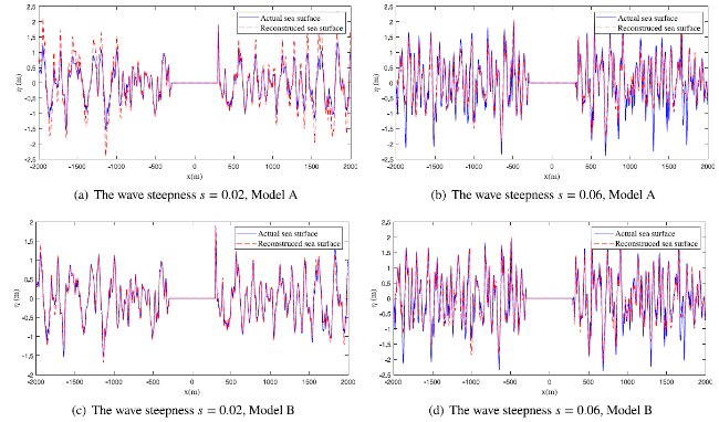
Fig. 6. The comparison between the reconstructed and actual wave elevation of the cross-section at y=0. The results of Model A and Model B with wave steepness levels of 0.02 and 0.06 are presented. |
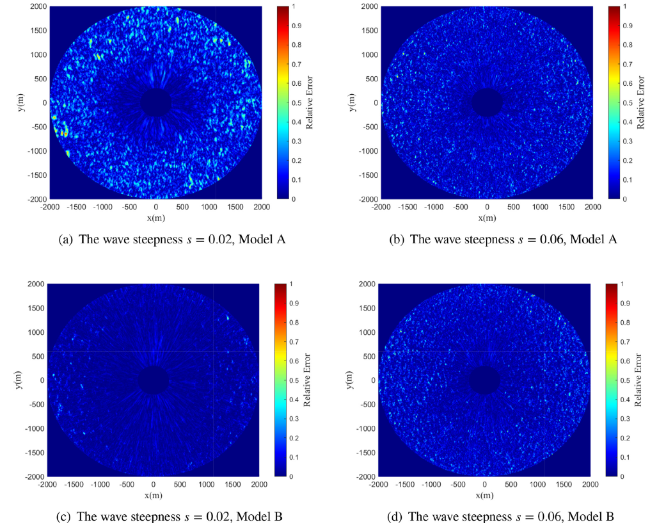
Fig. 7. The relative error at various wave steepness levels. The results of Model A and Model B with wave steepness levels of 0.02 and 0.06 are presented. |
To address this issue, we expanded the training data by generating radar images at wave steepness values of s=0.02,0.03,0.05, and 0.06, with $T_p$ ranging from 8.55s to 9.95s for s=0.02 and 0.03, and $T_p$ ranging from 6.05s to 7.45s for s=0.05 and 0.06. Thirty images were generated at each sea state when steepness s=0.04,0.06. Twenty images were generated at each sea state when steepness s=0.03,0.05 because these values are close to s=0.04. To demonstrate the model’s reliance on the training data, three training datasets were established: the first dataset (Dataset 1) contains data with wave steepness values of s=0.04, the second dataset (Dataset 2) contains data with wave steepness values of s=0.02,0.04, and 0.06, the third dataset (Dataset 3) contains data with wave steepness values of s=0.02,0.03,0.04,0.05 and 0.06. After training the CNN-based model with different training datasets, as shown in Table 5, Model A refers to the model trained with Dataset 1, Model B refers to the model trained with Dataset 2, and Model C refers to the model trained with Dataset 3.
Table 5. Models with different training data. |
| Models | Model A | Model B | Model C |
|---|---|---|---|
| Training datasets | Dataset 1 | Dataset 2 | Dataset 3 |
| Wave steepness in training data | 0.04 | 0.02,0.04,0.06 | 0.02,0.03,0.04,0.05,0.06 |
| Total samples | 3075 | 3975 | 4575 |
The results are shown in Fig. 8 and Table 6. In Fig. 8, the blue lines with circles represent results at wave steepness s=0.02; The red lines with squares represent results at wave steepness s=0.03; The green lines with crosses represent results at wave steepness s=0.05; The black lines with stars represent results at wave steepness s=0.06. We can see that the NDRMSE of the smaller wave steepness (s=0.02) data reduced to 0.04 for Model B, and 0.0414 for Model C. And the Corr increased to 0.9869 and 0.9861, respectively. From the comparison of Figs. 8(a), (c) and (e), we can see that the Corr of the model trained by the expanded data set is more stable. The Corr of the data with higher wave steepness (s=0.06) is improved slightly: from 0.9405 to 0.9482. Figs. 6(c) and Figs. 6(d) show the comparison of the wave elevation of Model B. It can be seen that when the wave steepness is 0.02, the consistency between the reconstructed sea surface and the actual sea surface is improved significantly. For wave steepness is 0.06, the consistency is improved, but the reconstructed wave elevation at the wave trough is still inconsistent with the actual wave elevation. Figs. 7(c) and Figs. 7(d) show the relative error of Model B, and the relative error of wave steepness of 0.02 decreased more than that of wave steepness of 0.06. For s=0.03 and s=0.05, the accuracy is hard to improve because the data are close to Dataset 1(s=0.04) and the accuracy is already high. For all the models, the accuracy decreases as the wave steepness increases. The difference between Model B and Model C shows that the U-Net model performs slightly better when trained with Dataset 2. This means that the model is better trained with fewer data with wider wave steepness intervals.
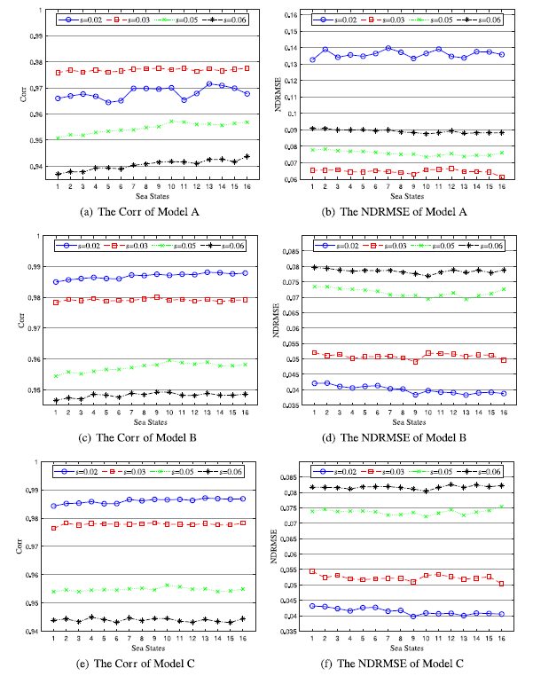
Fig. 8. The reconstruction outcomes with varying training data. |
Table 6. The reconstruction outcomes under varying wave steepness levels using different models. |
| Wave steepness | Model A | Model B | Model C | |||
|---|---|---|---|---|---|---|
| Corr | NDRMSE | Corr | NDRMSE | Corr | NDRMSE | |
| 0.02 | 0.9681 | 0.1360 | 0.9869 | 0.0400 | 0.9861 | 0.0414 |
| 0.03 | 0.9769 | 0.0647 | 0.9791 | 0.0509 | 0.9778 | 0.0523 |
| 0.05 | 0.9546 | 0.0757 | 0.9573 | 0.0715 | 0.9547 | 0.0736 |
| 0.06 | 0.9405 | 0.0891 | 0.9482 | 0.0785 | 0.9439 | 0.0817 |
4.3. Influence of sea state parameters on CNN-based model
As we can see from the previous section, changes in $H_s$ and $T_p$ may have varying effects on the model. Therefore, in this section, we investigate the trend of reconstruction accuracy as one parameter changes while the other remains fixed. Firstly, we generate three test sets of radar images with $T_p=6s,8s,10s$ and $H_s$ ranging from 2.2m to 6.07m with 0.43m increments. Then, we generate another three test sets of radar images with Hs=2.2m,4.2m,6.2m and $T_p$ ranging from 6s to 9.87s with 0.43s increments. Ten images are produced for each $T_p$ and $H_s$ pair. Given that the previous models are trained with data under fixed wave steepness, which means that $H_s$ and $T_p$ change simultaneously, it is necessary to broaden the data range to eliminate the impact of training data on the outcomes. The expanded training data are presented in Fig. 9. $T_p$ ranges from 6s to 10s with 0.1s increments, and $H_s$ ranges from 2.2m to 6.2m with 0.2m increments. With one image generated at each sea state, there are 861 images in total for the expanded training data. We observe that the parameter ranges of the expanded training data encompass the test data employed in this section.
The test results of the model trained with expanded training data are shown in Figs. 10 and 11. It is evident that there is a certain pattern in the performance of the model as the sea state parameters change: when $T_p$ is fixed, the reconstruction accuracy declines as the significant wave height increases; And when $H_s$ is fixed, the reconstruction accuracy increases as the peak wave period increases. In order to explain the cause of this phenomenon, radar images in four typical sea states are shown in Fig. 12. The parameters of the four typical sea states are $ T_{p}=10 \mathrm{~s}, H_{s}=2.2 \mathrm{~m} ; T_{p}=10 \mathrm{~s}, H_{s}=6.07 \mathrm{~m} $; $ T_{p}=6 \mathrm{~s}, H_{s}=2.2 \mathrm{~m} $ and $ T_{p}=6 \mathrm{~s}, H_{s}=6.2 \mathrm{~m} $.
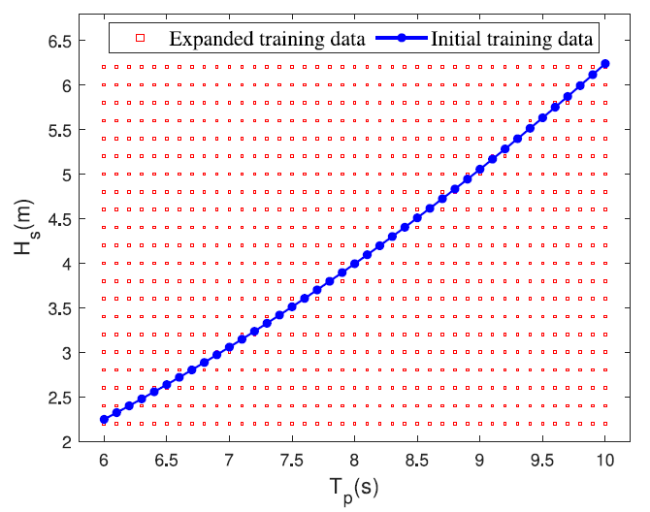
Fig. 9. The expanded training data. |
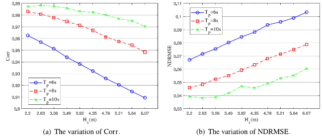
Fig. 10. Variation of Corr and NDRMSE with a fixed $T_p$. |
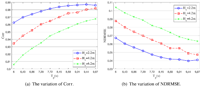
Fig. 11. Variation of Corr and NDRMSE with a fixed $H_s$. |
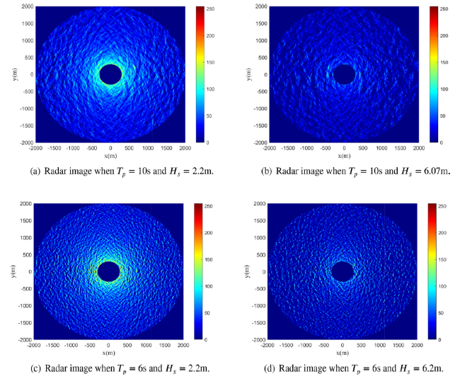
Fig. 12. Radar images in four typical sea states. |
As evident from the radar images, the significant wave height primarily affects the shaded regions while the peak wave period determines the wavelength. When the significant wave height increases, the shaded areas become more pronounced. Consequently, there is less wave information retained in the image, and the signal intensity weakens. Although the CNN-based model can discern wave information in shaded areas, the accuracy tends to decrease as the shaded area expands. The relative error maps in Fig. 13 demonstrate that the error is greater in shaded areas. The shading modulation frequently occurs in the wave trough, indicating that it is challenging for the CNN-based model to reconstruct wave elevation in wave troughs. Nonetheless, the radar signal is usually stronger in the wave crest, which facilitates easier reconstruction in those regions.
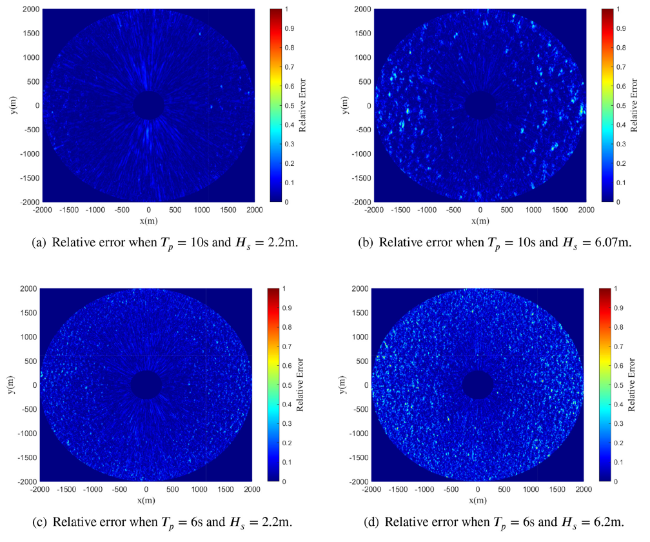
Fig. 13. Relative error in four typical sea states. |
As is apparent from the comparison of Figs. 12(a) and (c), as the peak period increases, so does the wavelength, resulting in noticeable differences in the wave patterns in radar images. The results suggest that the CNN-based model performs better when larger values of $T_p$, implying that the network’s architecture is better equipped to reconstruct the sea surface with longer wavelengths. When the wavelength is small, the texture of the wave becomes more intricate and detailed, making it challenging for the network to recognize and reconstruct the small wave. As can be seen from the comparison between Figs. 13(a) and (c), the relative error in the entire area with small peak period or wavelength is higher. A small significant wave height and a large perk period indicate low wave steepness. As shown in Table 6, the accuracy is higher when the wave steepness is low.
Although the accuracy has fluctuated, the Corr remains between the range of 0.90 to 0.99, and the NDRMSE remains between 0.03−0.11. For the test data in Fig. 10, the significant wave height ranges from 2.2m to 6.07m, and for Fig. 11, the peak period ranges from 6s to 9.87s. The model can ensure that the correlation coefficient is above 0.9 in such a wide range of wave parameters, and even reaches 0.988 in some sea states.
5. Conclusions
In this paper, we employed a deep learning model to reconstruct sea surfaces from radar images. The conventional method is based on spectral analysis, which may be limited by the assumption of linear wave theory and empirical parameters. In contrast, deep learning models, especially the CNN model, can tackle complex image problems. Hence, we proposed a new reconstruction method based on CNN. To achieve the image task’s goal, we chose U-Net, which is an image-to-image network, as the network structure.
Firstly, we compare the reconstruction outcomes of the conventional method and the CNN-based model U-Net. The CNN-based model exhibits significantly higher Corr and lower NDRMSE. Furthermore, in varying sea states and ranges, the CNN-based model displays greater stability. This not only demonstrates the practicability of employing the CNN-based model for sea surface reconstruction from radar images but also highlights the potential for higher accuracy using the CNN-based model.
Since the CNN-based model is a data-driven approach, we conducted several experiments to evaluate the model’s performance on various datasets. The training data primarily propagates in the θp=0∘ direction. However, by introducing random rotations to the image before the training process, the U-Net model can perform exceptionally well in different directions. Subsequently, the model was tested under varying wave steepness. Due to the test data’s distribution being beyond the training data, the accuracy dropped, although the Corr remained above 0.94, but the NDRMSE exceeded 0.13. To address this issue, we generated additional training data with varying wave steepness to train the model. With the expanded training data, the NDRMSE reduced by 0.096, and the maximum increase in Corr was 0.019.
Finally, we investigate the impact of significant wave height and peak period on the CNN-based model. The findings reveal that when the peak period remains constant, the accuracy decreases as the significant wave height increases, and when the significant wave height remains constant, the accuracy improves as the peak period increases. Although the accuracy fluctuates, the Corr remains above 0.90, and the NDRMSE remains less than 0.11.
Nonetheless, all experiments are carried out using synthetic radar images in this paper. It is essential to verify whether the CNN-based model is suitable for actual radar images. Meanwhile, for real waves, due to the second-order bound waves, the trough will be flatter compared to the linear wave model that was used in our experiments, thus the shadowing effect will be less severe which suggests that the performance of the CNN might be slightly better. Moreover, in reality, measuring actual sea surface elevation maps is challenging, implying that the label in the training data can only be acquired through other reconstruction methods or equipment. Thus, the quality of the label may impact the CNN-based model. Obtaining high-quality labels and applying the CNN-based model in practice will be crucial aspects of our subsequent study.
CRediT authorship contribution statement
Mingxu Zhao: Writing - original draft, Software, Data curation. Yaokun Zheng: Writing - review & editing, Software, Data curation. Zhiliang Lin: Conceptualization, Writing - review & editing.
Declaration of competing interest
The authors declare that they have no known competing financial interests or personal relationships that could have appeared to influence the work reported in this paper.
Acknowledgments
The authors acknowledge support from the National Natural Science Foundation of China (grant no. 51979162 and no. 52088102) and the Fundamental Research Funds for the Central Universities of China. This research was also sponsored by the Oceanic Interdisciplinary Program of Shanghai Jiao Tong University (project number SL2021MS019).
Appendix A. Influence of rescaling and noise
The last two steps of generating radar images are rescaling the $\sigma_{\text {tilt }}$ values to 256 gray levels and adding white Gaussian noise. The purpose of rescaling is to simulate the real radar images which are 256 gray level images according to [6], [7]. We denote the results of converting the $\sigma_{\text {tilt }}$ values to 256 gray levels without noise and the results of converting to 256 gray levels with noise as $ \sigma_{\text {no_noise }} $ and $ \sigma_{\text {noise }} $, respectively. To justify that converting $\sigma_{\text {tilt }}$ to a grayscale with only 256 levels will not have a significant impact on the predictions, we calculate the NDRMSE between the original intensity ($\sigma_{\text {tilt }}$) and rescaled intensities ($ \sigma_{\text {no_noise }} $ and $ \sigma_{\text {noise }} $) to measure the difference between them. Fig. A1 depicts $\sigma_{\text {tilt }}$, $ \sigma_{\text {no_noise }} $ and $ \sigma_{\text {noise }} $. From Fig. A1, it can be seen that the distribution of these three intensities is almost consistent, but the amplitudes are different due to the rescaling. Thus, to correctly compare these values, we need to rescale the rescaled intensities back to the range of the original intensity. The results are shown in Table A1. The NDRMSE between $\sigma_{\text {tilt }}$ and rescaled intensities is much smaller than the prediction which indicates that rescaling will not increase prediction error significantly. Meanwhile, it can be interpreted that the CNN-based model will learn the scaling mechanism from the data.
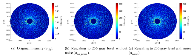
Fig. A1. Different intensity values. |
Table A1. NDRMSE between rescaled intensities and the original intensity, and the NDRMSE of CNN prediction. |
| $\sigma_{\text {no noise }}\left(\sigma_{\text {tilt }}+\text { rescale }\right)$ | $\sigma_{\text {noise }}\left(\sigma_{\text {tilt }}+\right.\text { rescale } \text { + noise) }$ | CNN prediction | |
|---|---|---|---|
| NDRMSE | 0.0001 | 0.0022 | 0.0624 |
