
1. Introduction
Internal solitary and periodic waves commonly exist in the density transition layer of real ocean, which causes reverse shear flow destroying the marine engineering structures nearby, such as fatigue damage to the risers of a spar platform caused by internal waves with large amplitudes [1], [2]. Therefore, it is necessary to study the internal wave loads on structures in order to reduce the destruction.
Two-layer fluid model with fixed densities of the upper and lower layers is a reasonable approximation of the continuous stratified water below sea level, which is widely applied in the internal wave problems. Internal waves in a two-layer fluid are usually called as interfacial waves.
The riser of a marine structure is often regarded as a cylindrical pile when computing the corresponding wave loads. The forces and torques on cylinders induced by internal waves is an interesting research area [3], [4], where much attention has been focused on internal solitary wave loads rather than on internal periodic wave loads.
For internal solitary wave loads, Cai et al. [3] calculated wave forces on cylinders by the classical Morison’s empirical formula [5] and concluded that detailed observation data of current provides accurate estimation. Cai et al. [6] further emphasized that wave force exerted by the first mode of internal solitary waves is much bigger than the rest of modes, and proposed an simpler wave force computation method. Then [7] considered loads of the internal solitary wave and shear flow on cylindrical piles, and found that the shear flow leads to a substantial increase of the wave loads. Xie et al. [8] conducted numerical simulations of wave forces and found that the force produced by tidal current on a cylindrical pile can be neglected compared with that caused by internal solitons. Si et al. [9] indicated that the crest of shear force on a cylinder locates at the zero point of horizontal velocity in an internal solitary wave system. Cai et al. [10] computed the wave loads on a cylindrical pile exerted by various internal solitary waves in different vertical distributions of density resulting from the seasonal variation. Based on the experiment research, Wang et al. [11] obtained coefficients of drag and inertial forces by the classical Morison equation and proposed a new Keulegan-Carpenter number. For internal solitary wave forces on a cylindrical pile, Zan and Lin [12] proposed a modified Morison’s formula and confirmed that the forces predicted by the modified Morison equation are more accurate than those evaluated by the classical one. Lin and Zan [4] proved the significance of convective acceleration in the modified Morison’s formula [12] on the loads of internal solitary waves.
For internal periodic wave loads, Ye and Shen [13] calculated the forces on a cylindrical pile based on linear wave solutions by the classical Morison equation, and found that the internal wave load of tidal frequency is of the same order of magnitude as the internal wave load of high frequency. Xu et al. [14] considered the interaction between a horizontal cylinder and internal periodic waves by experiment, and found that the horizontal drag force in the density transition layer is smaller compared with the force outside the corresponding layer. Wang et al. [15] experimentally studied the internal periodic wave forces on several vertical cylinders distributed in various depths, and emphasized that cyclic shear load can lead to fatigue damage. For the loads on a vertical cylinder with a plate, Lin et al. [16] considered the wave system governed by linearized potential flow theory, and found that the plate enlarges the horizontal loads on the cylindrical pile. Li et al. [17] theoretically investigated the fully nonlinear interfacial wave loads on a cylinder with a rigid upper surface by the classical Morison’s formula, and obtained more accurate results of the wave loads than previously ones based on the linear or weakly nonlinear wave solutions.
So far, most previously theoretical studies about the interfacial or internal periodic wave loads on vertical cylindrical piles were based on linear or weakly nonlinear wave model, with only a few research work considered the fully nonlinear wave model (see e.g. Li et al. [17]). Until now, the fully nonlinear interfacial periodic waves in a two-layer fluid with free surface have not been obtained theoretically, and the loads estimation of the nonlinear interfacial waves by the modified Morison equation [12] have not been studied, too.
This paper investigates interfacial periodic gravity waves on the basis of fully nonlinear potential flow equations including the free-surface boundary conditions, and evaluates the wave forces on a cylinder in a two-layer fluid. For internal waves in the real ocean, the density ratio between upper and lower fluid layers is a constant near 1. Hence we only consider the Boussinesq wave forces [18] here. The wave steepness of free surface and internal interface, surface and interface wave profiles and corresponding forces on a cylinder are analysed with different nonlinearities, upper and lower layer depths.
The homotopy analysis method (HAM) [19], [20], [21], [22], an analytic approximation method for nonlinear ODE and PDE, is applied in this paper to obtain convergent series solutions of interfacial periodic gravity waves. The wave forces on the cylindrical pile are predicted by the classical [5] and the modified [12] Morison’s formulae.
The contributions of this paper are summarized as follows: firstly, we develop the solution procedure in the HAM for a fully nonlinear interfacial periodic wave model from the rigid upper boundary [17] to the free-surface boundary conditions. Compared with the physical model with fixed upper surface, the model with free surface represents better the real ocean environment; secondly, wave forces on a cylindrical pile are estimated by both the classical and modified Morison equations. The investigation of wave forces on a cylinder evaluated by the modified Morison formula is extended from the internal solitary waves to the interfacial periodic waves; finally, the total inertial forces or global forces predicted by the classical and modified Morison equations are analyzed for various physical parameters.
The structure of this paper is: Section 2 shows the mathematical description of the governing equations of nonlinear interfacial periodic waves, related solution procedures in the HAM, and the classical and modified Morison equations. Section 3 analyzes the results for wave forces on a cylinder with the variation of nonlinearity, upper and lower layer depths. Section 4 concludes the main findings.
2. Mathematical formulae
2.1. Governing equations
We consider a system of two inviscid, incompressible fluid layers with constant densities under gravity. The upper layer, with $h_1$ thickness, has a free surface. Depth of the lower layer is $h_2$. The flow is assumed irrotational inside each fluid layer. Figure 1 illustrates the layered system for densities $\rho_{1}<\rho_{2}$. Here $(x,y,z)$ represents the Cartesian coordinate system, in which $z=0$ and $z=−h_1$ are horizontal planes located at the undisturbed free surface and interface between the fluid layers, respectively. z is measured vertically upwards. The governing equations for both layers read
$\nabla^{2} \phi_{1}=0, \quad-h_{1}+\zeta_{2}<z<\zeta_{1}$
$\nabla^{2} \phi_{2}=0, \quad-h_{1}-h_{2}<z<-h_{1}+\zeta_{2}$
subject to kinematic and dynamic boundary conditions at the free surface $z=\zeta_{1}$
$\frac{\partial^{2} \phi_{1}}{\partial t^{2}}+g \frac{\partial \phi_{1}}{\partial z}+\frac{\partial\left(\left|\nabla \phi_{1}\right|^{2}\right)}{\partial t}+\nabla \phi_{1} \cdot \nabla\left(\frac{1}{2}\left|\nabla \phi_{1}\right|^{2}\right)=0$
$\zeta_{1}+\frac{1}{g}\left(\frac{\partial \phi_{1}}{\partial t}+\frac{1}{2}\left|\nabla \phi_{1}\right|^{2}\right)=0$
kinematic and dynamic boundary conditions at the interface $z=-h_{1}+\zeta_{2}$
$ \begin{aligned} \frac{\partial^{2} \phi_{2}}{\partial t^{2}} & +g(1-\Delta) \frac{\partial \phi_{2}}{\partial z}-\Delta \frac{\partial^{2} \phi_{1}}{\partial t^{2}}+\frac{\partial\left(\left|\nabla \phi_{2}\right|^{2}\right)}{\partial t}-\Delta \frac{\partial\left(\frac{1}{2}\left|\nabla \phi_{1}\right|^{2}\right)}{\partial t} \\ & +\nabla \phi_{2} \cdot \nabla\left(\frac{1}{2}\left|\nabla \phi_{2}\right|^{2}\right)-\Delta \nabla \phi_{2} \cdot \nabla\left(\frac{\partial \phi_{1}}{\partial t}+\frac{1}{2}\left|\nabla \phi_{1}\right|^{2}\right)=0 \end{aligned}$
$\begin{aligned} g(1 & -\Delta) \frac{\partial\left(\phi_{2}-\phi_{1}\right)}{\partial z}+\frac{\partial\left(\frac{1}{2}\left|\nabla \phi_{2}\right|^{2}\right)}{\partial t}+\nabla \phi_{2} \cdot \nabla\left(\frac{1}{2}\left|\nabla \phi_{2}\right|^{2}\right) \\ & -\nabla \phi_{1} \cdot \nabla\left(\frac{\partial \phi_{2}}{\partial t}+\frac{1}{2}\left|\nabla \phi_{2}\right|^{2}\right)+\Delta\left[\frac{\partial\left(\frac{1}{2}\left|\nabla \phi_{1}\right|^{2}\right)}{\partial t}\right. \\ & \left.+\nabla \phi_{1} \cdot \nabla\left(\frac{1}{2}\left|\nabla \phi_{1}\right|^{2}\right)-\nabla \phi_{2} \cdot \nabla\left(\frac{\partial \phi_{1}}{\partial t}+\frac{1}{2}\left|\nabla \phi_{1}\right|^{2}\right)\right]=0 \end{aligned}$
$\zeta_{2}-\frac{1}{g(1-\Delta)}\left[\Delta\left(\frac{\partial \phi_{1}}{\partial t}+\frac{1}{2}\left|\nabla \phi_{1}\right|^{2}\right)-\left(\frac{\partial \phi_{2}}{\partial t}+\frac{1}{2}\left|\nabla \phi_{2}\right|^{2}\right)\right]=0$
and a kinematic boundary condition at the bottom $z=-h_{1}-h_{2}$
$\frac{\partial \phi_{2}}{\partial z}=0$
where $\phi_{1}(x, y, z, t)$ and $\phi_{2}(x, y, z, t)$ denote velocity potentials of the upper and lower fluid layers, $z=\zeta_{1}(x, y, t)$ is the free surface elevation and $z=-h_{1}+\zeta_{2}(x, y, t)$ is the interface level between the two layers, g is the acceleration due to gravity, t is time, $\Delta=\rho_{1} / \rho_{2}$ is the density ratio between the upper and lower layers, and $\nabla=e_{x} \frac{\partial}{\partial z}+e_{y} \frac{\partial}{\partial y}+e_{z} \frac{\partial}{\partial z}$ is the gradient operator. Appendix A presents a detailed derivation of the interface deformation conditions (5)–(7).
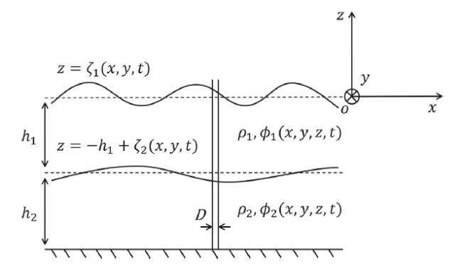
Fig. 1. The physical sketch of the two-fluid system with related notations.Consider a steady-state interfacial wave system with one primary periodic progressive wave component. Let $k$ denote the wave vector, $k=|k|$ the wave number, and $σ$ the actual angular frequency of the primary component. Since the amplitude of each component in a steady-state interfacial wave system is time-independent, the following transformation is introduced to eliminate the time variable t |
$\xi=\boldsymbol{k} \cdot \boldsymbol{r}-\sigma t$
where $r=e_{x} x+e_{y} y$, and define
$\varphi_{i}(\xi, z)=\phi_{i}(x, y, z, t), \quad \eta_{i}(\xi)=\zeta_{i}(x, y, t), \quad i=1,2$
in the new coordinate system $(\xi, z)$. The original initial/boundary-value problem (1)–(8) in the coordinate system $(x, y, z, t)$ is then transformed into a boundary-value problem in the coordinate system $(\xi, z)$. The governing equations in the coordinate system $(\xi, z)$ are
$\widehat{\nabla}^{2} \varphi_{1}=0, \quad-h_{1}+\eta_{2}<z<\eta_{1}$
$\widehat{\nabla}^{2} \varphi_{2}=0, \quad-h_{1}-h_{2}<z<-h_{1}+\eta_{2}$
subject to two (one kinematic and one dynamic) boundary conditions at the unknown free surface $z=\eta_{1}$
$\mathscr{N}_{1}\left[\varphi_{1}\right]=\sigma^{2} \frac{\partial^{2} \varphi_{1}}{\partial \xi^{2}}+g \frac{\partial \varphi_{1}}{\partial z}-2 \sigma \frac{\partial f_{1}}{\partial \xi}+\widehat{\nabla} \varphi_{1} \cdot \widehat{\nabla} f_{1}=0$
$\mathscr{N}_{2}\left[\varphi_{1}, \eta_{1}\right]=\eta_{1}-\frac{1}{g}\left(\sigma \frac{\partial \varphi_{1}}{\partial \xi}-f_{1}\right)=0$,
three (two kinematic and one dynamic) boundary conditions at the unknown interface $z=-h_{1}+\eta_{2}$
$\begin{array}{l} \mathscr{N}_{3}\left[\varphi_{1}, \varphi_{2}\right]=\sigma^{2} \frac{\partial^{2} \varphi_{2}}{\partial \xi^{2}}+g(1-\Delta) \frac{\partial \varphi_{2}}{\partial z}-\Delta \sigma^{2} \frac{\partial^{2} \varphi_{1}}{\partial \xi^{2}}+\widehat{\nabla} \varphi_{2} \cdot \widehat{\nabla} f_{2} \\ -2 \sigma \frac{\partial f_{2}}{\partial \xi}+\Delta\left(\sigma \frac{\partial f_{1}}{\partial \xi}-h_{21}-\widehat{\nabla} \varphi_{2} \cdot \widehat{\nabla} f_{1}\right)=0 \end{array}$
$\begin{aligned} \mathscr{N}_{4}\left[\varphi_{1}, \varphi_{2}\right] & =g(1-\Delta) \frac{\partial\left(\varphi_{2}-\varphi_{1}\right)}{\partial z} \\ & +\widehat{\nabla}\left(\varphi_{2}-\varphi_{1}\right) \cdot \widehat{\nabla} f_{2}-h_{12}-\sigma \frac{\partial f_{2}}{\partial \xi}-\Delta\left[\sigma \frac{\partial f_{1}}{\partial \xi}+h_{21}\right. \\ & \left.+\widehat{\nabla}\left(\varphi_{2}-\varphi_{1}\right) \cdot \widehat{\nabla} f_{1}\right]=0 \end{aligned}$
$\mathscr{N}_{5}\left[\varphi_{1}, \varphi_{2}, \eta_{2}\right]=\eta_{2}-\frac{1}{g(1-\Delta)}\left[\sigma \frac{\partial \varphi_{2}}{\partial \xi}-f_{2}-\Delta\left(\sigma \frac{\partial \varphi_{1}}{\partial \xi}-f_{1}\right)\right]=0$
and a bottom boundary condition
$\frac{\partial \varphi_{2}}{\partial z}=0, \quad z=-h_{1}-h_{2}$
where $\mathscr{N}_{i}$ with i=1,2,...,5 are nonlinear differential operators and
$\widehat{\nabla}=\boldsymbol{k} \frac{\partial}{\partial \xi}+\boldsymbol{e}_{z} \frac{\partial}{\partial z}, \quad f_{i}=\frac{1}{2}\left|\widehat{\nabla} \varphi_{i}\right|^{2}, \quad i=1,2$
$h_{i j}=-\sigma \widehat{\nabla} \varphi_{i} \cdot \widehat{\nabla}\left(\frac{\partial \varphi_{j}}{\partial \xi}\right), \quad i, j=1,2$
The disturbed free surface elevation$η_1$, the disturbed interface elevation $η_2$, and the velocity potentials in the upper and lower fluid layers $φ_i$ of the steady-state interfacial wave system can be expressed in the form
$\eta_{1}(\xi)=\sum_{i=0}^{+\infty} C_{i}^{\eta_{1}} \cos (i \xi)$
$\eta_{2}(\xi)=\sum_{i=0}^{+\infty} C_{i}^{\eta_{2}} \cos (i \xi)$
$\varphi_{1}(\xi, z)=\sum_{i-1}^{+\infty}\left(C_{i}^{\varphi_{1 a}} \psi_{i}^{1 a}+C_{i}^{\varphi_{1 b}} \psi_{i}^{1 b}\right)$
$\varphi_{2}(\xi, z)=\sum_{i=1}^{+\infty} C_{i}^{\varphi_{2}} \psi_{i}^{2}$
in which
$\psi_{i}^{1 a}(\xi, z)=\cosh \left[k_{i}\left(z+h_{1}\right)\right] \sin (i \xi)$
$\psi_{i}^{1 b}(\xi, z)=\sinh \left[k_{i}\left(z+h_{1}\right)\right] \sin (i \xi)$
$\psi_{i}^{2}(\xi, z)=\cosh \left[k_{i}\left(z+h_{1}+h_{2}\right)\right] \sin (i \xi)$
with the definition $k_{i}=|i \boldsymbol{k}|.$ In all cases, prescribed values of $\Delta, \boldsymbol{k}, \sigma, h_{1}$ and $h_2$ are used to determine the otherwise unknown constants $C_{i}^{\eta_{1}}, C_{i}^{\eta_{2}}, C_{i}^{\varphi_{12}}, C_{i}^{\varphi_{18}}$ and $C_{i}^{\varphi_{2}}$ as follows. Eqs. (11), (12) and (18) are automatically satisfied by the form of $η_i$ and $φ_i$ given by (21)–(24), and the unknown constants are hence obtained by solving the two boundary conditions (13) and (14) at the free surface $z=\eta_{1}$ and the three boundary conditions (15)–(17) at the internal interface $z=-h_{1}+\eta_{2}$.
2.2. Approach based on the HAM
The general idea behind the homotopy analysis method (HAM) is the continuous deformation of initial guesses in achieving the solutions of nonlinear differential equations. Comprehensive introductions to the HAM are given by Liao [19], [20]. The fundamental concept and important details of the HAM are briefly summarised below.
Given that the expressions for $φ_1$ (23) and $φ_2$ (24) automatically satisfy the governing Eqs. (11) and (12) and boundary condition (18), it is sufficient solely to consider the free surface and interface conditions (13)–(17). We set q∈[0,1] as an embedding homotopy parameter, $c_0≠0$ as a convergence-control parameter, and $\mathscr{L}_{i}$ with i=1,3,4 as the auxiliary linear operators. Besides, $\eta_{0,1}=\eta_{0,2}=0$ are taken to be initial approximations of vertical disturbances to the free surface $η_1$ and the interface $η_2$, and $\varphi_{0,1}(\xi, z)$ and $\varphi_{0,2}(\xi, z)$ as initial approximations of the potential functions $φ_1$ and $φ_2$. Then, based on the free surface and interface conditions (13)–(17), we construct the following parameterized family of equations (called the zeroth-order deformation equations):
$(1-q) \mathscr{L}_{1}\left[\check{\varphi}_{1}-\varphi_{0,1}\right]=q c_{0} \mathscr{N}_{1}\left[\check{\varphi}_{1}\right], \quad \text { at } z=\check{\eta}_{1},$
$(1-q) \check{\eta}_{1}=q c_{0} \mathscr{N}_{2}\left[\breve{\varphi}_{1}, \check{\eta}_{1}\right], \quad \text { at } z=\check{\eta}_{1}$
$(1-q) \mathscr{L}_{3}\left[\check{\varphi}_{1}-\varphi_{0,1}, \check{\varphi}_{2}-\varphi_{0,2}\right]=q c_{0} \mathscr{N}_{3}\left[\check{\varphi}_{1}, \breve{\varphi}_{2}\right] ; \quad \text { at } z=-h_{1}+\check{\eta}_{2} \text {, }$
$(1-q) \mathscr{L}_{4}\left[\check{\varphi}_{1}-\varphi_{0,1}, \check{\varphi}_{2}-\varphi_{0,2}\right]=q c_{0} \mathscr{N}_{4}\left[\check{\varphi}_{1}, \breve{\varphi}_{2}\right] ; \quad \text { at } z=-h_{1}+\check{\eta}_{2}$
$(1-q) \check{\eta}_{2}=q c_{0} \mathscr{N}_{5}\left[\breve{\varphi}_{1}, \breve{\varphi}_{2}, \breve{\eta}_{2}\right], \quad \text { at } z=-h_{1}+\breve{\eta}_{2}$
where
$\check{\varphi}_{i}(\xi, z ; q)=\sum_{n=0}^{+\infty} \varphi_{n, i} q^{n}, \quad \varphi_{n, i}(\xi, z)=\left.\frac{1}{n!} \frac{\partial^{n} \check{\varphi}_{i}}{\partial q^{n}}\right|_{q 0}, \quad i=1,2$
$\check{\eta}_{i}(\xi ; q)=\sum_{n=1}^{+\infty} \eta_{n, i} q^{n}, \quad \eta_{n, i}(\xi)=\left.\frac{1}{n!} \frac{\partial^{n} \check{\eta}_{i}}{\partial q^{n}}\right|_{q=0}, \quad i=1,2$
Considering the auxiliary linear operators $\mathscr{L}_{i}$ which have the property $\mathscr{L}_{1}[0]=\mathscr{L}_{3}[0,0]=\mathscr{L}_{4}[0,0]=0$, we obtain the following relationships when $q=0$:
$\breve{\varphi}_{i}(\xi, z ; 0)=\varphi_{0, i}, \quad \check{\eta}_{i}(\xi ; 0)=0, \quad i=1,2.$
When $q=1$, Eqs. (28)–(32) are equivalent to the original Eqs. (13)–(17), respectively. Thus
$\breve{\varphi}_{i}(\xi, z ; 1)=\varphi_{i}, \quad \check{\eta}_{i}(\xi ; 1)=\eta_{i}, \quad i=1,2$
Hence, (28)-(32) define four homotopies:
$\check{\varphi}_{i}:=\varphi_{0, i} \sim \varphi_{i} ; \quad \check{\eta}_{i}:=0 \sim \eta_{i}, \quad \text { when } q:=0 \sim 1, \quad i=1,2$
Letting $q=1$, the solutions for disturbed free surface and interface $η_i$ and velocity potentials in the upper and lower fluid layers $φ_i$ are expressed by
$\eta_{i}(\xi)=\breve{\eta}_{i}(\xi ; 1)=\sum_{m=1}^{+\infty} \eta_{m, i}(\xi), \quad i=1,2$
$\varphi_{i}(\xi, z)=\breve{\varphi}_{i}(\xi, z ; 1)=\sum_{m=0}^{+\infty} \varphi_{n, \dot{i}}(\xi, z), \quad i=1,2$
The sum indexes of $η_1$ and $η_2$ commence from $m=1$ because the initial guesses $\eta_{0,1}=\eta_{0,2}=0$.
2.2.1. Solution procedure
The unknown $φ_{m,i}$ and $η_{m,i}$ are governed by the high-order deformation equations(40)L‾1[φm,1]=c0Δm−1,1φ+χm(Sm−1,1−S‾m,1),m≥1,(41)L‾i+1[φm,1,φm,2]=c0Δm−1,iφ+χm(Sm−1,i−S‾m,i),i=2,3,m≥1,(42)ηm,i=c0Δm−1,iη+χmηm−1,i,i=1,2,m≥1,in which χ1=0 and χm=1 for m≥2; L‾1=L1|z=0, L‾3=L3|z=−h1, and L‾4=L4|z=−h1 are auxiliary linear operators.
Up to the mth-order of approximation, all of the terms Δm−1,iφ, S‾m,i, Sm−1,i and Δm−1,iη on the right side of the high-order deformation Eqs. (40)-(42) have been already predetermined by φn,i and ηn,i, with n=0,1,2,…,m−1 and m≥1. More detailed expressions for the high-order deformation Eqs. (40)-(42) are provided in Appendix B and the next section. Although ηm,1 and ηm,2 can be obtained directly from (42), to obtain the expressions of φm,1 and φm,2 needs to solve coupled Eqs. (40) and (41) with the solving process shown in the next section.
2.2.2. Choice of auxiliary linear operators
The model given by Eqs. (11)-(18) has two modes corresponding to different linear dispersion relationships. Linear angular frequency for surface wave mode(43)ωS(ki)=gkiCT1+CT2+(CT1+CT2)2−4(1−Δ)(Δ+CT1CT2)2(Δ+CT1CT2),and linear angular frequency for internal wave mode(44)ωI(ki)=gkiCT1+CT2−(CT1+CT2)2−4(1−Δ)(Δ+CT1CT2)2(Δ+CT1CT2),in which CT1=coth(kih1) and CT2=coth(kih2). Referring to the linear parts of Eqs. (13), (15) and (16), we choose the following auxiliary linear operators(45)L1[φ1]=ω2∂2φ1∂ξ2+g∂φ1∂z,(46)L3[φ1,φ2]=ω2∂2φ2∂ξ2+g(1−Δ)∂φ2∂z−Δω2∂2φ1∂ξ2,(47)L4[φ1,φ2]=g(1−Δ)(∂φ2∂z−∂φ1∂z),where ω=σ/ϵ denotes the linear angular frequency of the primary component corresponding to either ωS(k) or ωI(k), and ϵ denotes the dimensionless angular frequency. Since [23] found that the interfacial waves with ω=ωS(k) behave like surface gravity waves, ω=ωI(k) is chosen for all cases considered in this paper. For a wave system with components all travelling in the same direction, ϵ>1 and larger ϵ means greater nonlinearity. Expressions for Sm,i and S‾m,i can be obtained as(48)Sm,1=ω2β2,1,1m,0+gγ0,1,1m,0+S‾m,1,(49)S‾m,1=∑n=1m−1(ω2β2,1,1m−n,n+gγ0,1,1m−n,n),(50)Sm,2=ω2β2,2,2m,0+g(1−Δ)γ0,2,2m,0−Δω2β2,1,2m,0+S‾m,2,(51)S‾m,2=∑n=1m−1[ω2β2,2,2m−n,n+g(1−Δ)γ0,2,2m−n,n−Δω2β2,1,2m−n,n],(52)Sm,3=g(1−Δ)(γ0,2,2m,0−γ0,1,2m,0)+S‾m,3,(53)S‾m,3=∑n=1m−1[g(1−Δ)(γ0,2,2m−n,n−γ0,1,2m−n,n)],with detailed formulae of βi,k‾,pn,m and γi,k‾,pn,m shown in Appendix B. Following the series expressions (23) and (24), we define φm,1 and φm,2 in the general forms(54)φm,1=∑i(Ciφ1a,mψi1a+Ciφ1b,mψi1b),φm,2=∑iCiφ2,mψi2.The mth-order deformation Eqs. (40) and (41) are then simplified as(55)L‾1[∑i(Ciφ1a,mψi1a+Ciφ1b,mψi1b)]=∑iRi1,msin(iξ),(56)L‾3[∑i(Ciφ1a,mψi1a+Ciφ1b,mψi1b),∑iCiφ2,mψi2]=∑iRi3,msin(iξ),(57)L‾4[∑i(Ciφ1a,mψi1a+Ciφ1b,mψi1b),∑iCiφ2,mψi2]=∑iRi4,msin(iξ),where Ciφ1a,m, Ciφ1b,m and Ciφ2,m are all constants to be determined form the already known Ri1,m, Ri3,m and Ri4,m. Equating the terms on both sides of the Eqs. (55)-(57), the following three linear algebraic equations are obtained(58)gki[Ciφ1b,mcosh(kih1)+Ciφ1a,msinh(kih1)]−i2ω2[Ciφ1a,mcosh(kih1)+Ciφ1b,msinh(kih1)]=Ri1,m,(59)Ciφ2,m[gki(1−Δ)sinh(kih2)−i2ω2cosh(kih2)]+i2ω2ΔCiφ1a,m=Ri3,m,(60)gki(1−Δ)[Ciφ2,msinh(kih2)−Ciφ1b,m]=Ri4,m.The solutions for Ciφ1a,m, Ciφ1b,m and Ciφ2,m are(61)Ciφ1a,m=Ri3,m+[i2ω2cosh(kih2)−gki(1−Δ)sinh(kih2)]Ciφ2,mi2ω2Δ,(62)Ciφ1b,m=Ciφ2,msinh(kih2)−Ri4,mgki(1−Δ),(63)Ciφ2,m=DiRi1,m+AiRi3,m+BiRi4,m[Δ+coth(kih1)coth(kih2)]λiSλiI,where(64)Ai=1Δ[cosh(kih1)−gkisinh(kih1)i2ω2],(65)Bi=11−Δ[cosh(kih1)−i2ω2sinh(kih1)gki],(66)Di=−i2ω2Δsinh(kih1)sinh(kih2),(67)λiS=(iω)2−ωS2(ki),(68)λiI=(iω)2−ωI2(ki).For non-primary component cos(iξ), λiS and λiI are not small real numbers. Ciφ2,m can be obtained directly from (63), and Ciφ1a,m and Ciφ1b,m are then calculated from (61), (62). For the primary component cos(ξ), λ1Sλ1I=0. Therefore, C1φ2,m cannot be obtained directly from (63). Instead, to eliminate the singularity, we force the numerator of the right-hand side of (63) to be equal to 0, such that(69)R11,m+A1R13,m+B1R14,m=0,from which the value of C1φ2,m−1 is determined. Similarly, C1φ2,m is determined from the right-hand side of (63) via(70)R11,m+1+A1R13,m+1+B1R14,m+1=0.Once the value of C1φ2,m is determined, we can obtain C1φ1a,m and C1φ1b,m directly from (61), (62).
2.2.3. Choice of initial guesses
Based on the linearized solutions of Eqs. (11)-(18), we choose the following initial guesses(71)φ0,1=1Δ[cosh(kh2)−gk(1−Δ)ω2sinh(kh2)]C1φ2,0ψ11a+C1φ2,0sinh(kh2)ψ11b,(72)φ0,2=C1φ2,0ψ12,for velocity potentials and η0,1=η0,2=0 for disturbed free surface and interface elevations. When m=1, Eq. (69) is a nonlinear algebraic equation, from which unique value of |C1φ2,0| is determined. Without loss of generality, negative C1φ2,0 is chosen for all computed cases because the positive or negative value merely implies different initial phase in ξ (9). When m>1, Eq. (69) is a linear algebraic equation for C1φ2,m−1.
2.2.4. Choice of convergence-control parameter
In order to guarantee the convergence of series (38) and (39) to the solution of Eqs. (13)-(17), the following averaged residual squares are defined(73)ϵm=ϵmφ,1+ϵmφ,2+ϵmφ,3+ϵmη,1+ϵmη,2,in which(74)ϵmφ,i=12π∫02π(∑n=0mΔn,iφ)2dξ,i=1,2,3,represent the residuals of Eqs. (13), (15) and (16), respectively, and(75)ϵmη,i=12π∫02π(∑n=0mΔn,iη)2dξ,i=1,2,represent the residuals of Eqs. (14) and (17). Note that Δn,1φ, Δn,2φ, Δn,3φ, Δn,1η and Δn,2η could be obtained in the (n+1)th-order deformation Eqs. (40)-(42).
Figure 2 shows the averaged residual squares log10ϵm−1 and the convergence-control parameter c0 with different orders of approximation for ϵ=1.02. The residual in the range of −1.2<c0<0 decreases with the order of approximation increasing, and the value of c0 near the minimum point of each residual is chosen to accelerate the convergence of series solutions. Table 1 shows the corresponding amplitudes of wave components |Ciη1| and |Ciη2| and averaged residual squares ϵm−1 for c0=−0.8. The residual decreases as the order of approximation increases, and the wave amplitudes with three significant digits can be obtained up to the 41st-order approximation.
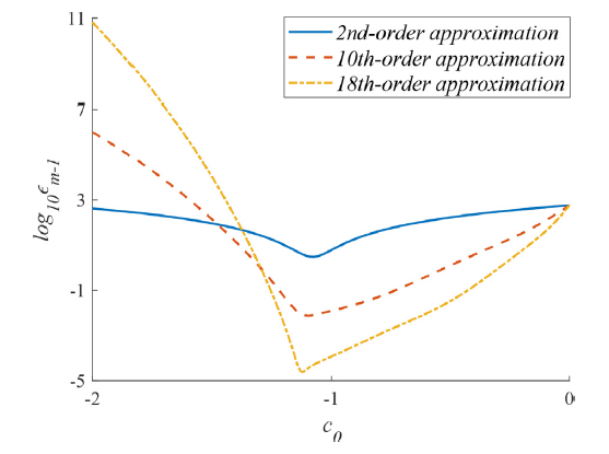
Fig. 2. Averaged residual squares versus convergence-control parameter in the case of,, and. Solid line for 2nd-order approximation, dashed line for 10th-order approximation, dash-dotted line for 18th-order approximation. |
Table 1. Amplitudes of wave components and |Ciη2| and averaged residual squares ϵm−1 in the case of kh1=0.942, kh2=12.566, Δ=0.996, ϵ=1.02 and c0=−0.8. |
| order | |C1η1|(m) | |C2η1|(m) | |C1η2|(m) | |C2η2|(m) | ϵm−1 |
|---|---|---|---|---|---|
| 1 | 0.0415 | 0.00192 | 26.5 | 0.477 | 5.77×10² |
| 11 | 0.0761 | 0.00893 | 47.4 | 5.19 | 2.93×10⁻² |
| 21 | 0.0773 | 0.00912 | 48.0 | 5.45 | 2.83×10⁻⁴ |
| 31 | 0.0774 | 0.00914 | 48.0 | 5.48 | 4.13×10⁻⁶ |
| 41 | 0.0775 | 0.00914 | 48.0 | 5.49 | 7.76×10⁻⁸ |
| 51 | 0.0775 | 0.00914 | 48.0 | 5.49 | 1.66×10⁻⁹ |
| 61 | 0.0775 | 0.00914 | 48.0 | 5.49 | 3.88×10⁻¹¹ |
To sum up, a suitable value of convergence-control parameter c0 can guarantee and accelerate the convergence of series solutions (38)-(39) to the Eqs. (13)-(17), and the choice of convergence-control parameters for all cases considered in this paper follows the same procedure as described in this subsection.
2.3. Wave forces evaluated by the classical and modified Morison equations
The classical Morison equation [5] and modified Morison equation [12] are used to estimate the forces on a cylindrical pile along the z-axis caused by Boussinesq periodic waves [18] in the case Δ=0.996. This pile is located in the coordinate (0,0,−h1−h2≤z≤ζ1(0,0,t)) as shown in Fig. 1. Letting λ=2π/k represent the wave length of the primary component, we assume that the diameter D of the pile is small enough and satisfied with D/λ≤0.15 to ensure that the interfacial wave field is undisturbed.
2.3.1. Classical Morison equation
Referring to Morison et al. [5] and Cai et al. [7], the wave force contains drag and inertial components. For a slice of the pile:(76)dFDi=12ρiCDDui|ui|dz,(77)dFIi=ρiCMπD24∂ui∂tdz,i=1,2,where dFD1 and dFI1 are upper layer drag and inertial forces, dFD2 and dFI2 are lower layer drag and inertial forces, CD and CM are hydrodynamic coefficients determined experimentally (see e.g. [7], [24], [25]), u1=∂ϕ1/∂x and u2=∂ϕ2/∂x are x− velocity components at (0,0,z) in upper and lower layers, respectively. Then a series of wave forces on the pile are obtained:(78)FD(t)=∫−h1+ζ2ζ1dFD1+∫−h1−h2−h1+ζ2dFD2,(79)FI(t)=∫−h1+ζ2ζ1dFI1+∫−h1−h2−h1+ζ2dFI2,(80)Fg(t)=FD+FI,where FD is the total drag force, FI the total inertial force, and Fg the global force. The above formulae of wave forces are based on the classical Morison Eq. (76) and (77).
2.3.2. Modified Morison equation
Zan and Lin [12] proposed a modified Morison equation which provides more accurate predictions of wave forces than the classical Morison equation, exerted by internal solitary waves on a cylinder. The difference between the classical and modified Morison equations results from the different derivatives of x− velocity component ui with respect to time t in the inertial force formula (77). Substantial derivative in the modified equation replaces the partial derivative in the classical equation, given by(81)dFIi′=ρiCMπD24duidtdz,i=1,2,(82)duidt=∂ui∂t+ui∂ui∂x+vi∂ui∂y+wi∂ui∂z,where (ui,vi,wi)=∇ϕi. The neglected convective acceleration in the classical Morison equation is re-added to the modified formula (81). By replacing (77) with (81), the wave forces based on the modified Morison equation are obtained following the same process in Section 2.3.1 with a prime in the upper right corner like FI′.
3. Results and discussion
Wave steepness of free surface Hs1 and internal interface Hs2 are defined as follows(83)Hsi=kmax[ηi(ξ)]−min[ηi(ξ)]2,ξ∈[0,2π],i=1,2,in which max[ηi(ξ)]−min[ηi(ξ)] denotes the maximal wave height.
The relative error between the total inertial forces estimated by the classical and modified Morison equations shown in Section 2.3 is defined as(84)reFI=||FI′|max−|FI|max||FI|max,and similarly, the relative error between the global forces estimated by the classical and modified Morison equations is(85)reFg=||Fg′|max−|Fg|max||Fg|max,where the “max” in the lower right corner represents the maximum value.
The fixed physical parameters for the fluid layers, interfacial waves and cylindrical pile in this paper are chosen as:(86)Δ=0.996,λ=2πk=1000(m),α=0,g=9.8(m·s−2),ρ1=1023.5(kg·m−3),ρ2=ρ1Δ,D=5(m),where D/λ=0.005<0.15, and α is the angle between the wave vector of the primary component k and the unit vector ex.
3.1. Wave forces with increased nonlinearity
First, we consider the effects of nonlinearity on interfacial waves and wave forces. Since the wave steepness is positively correlated with the dimensionless angular frequency $ϵ$ for a unidirectional wave system, the cases with increased ϵ are calculated.
Figure 3 presents the relationship between wave steepness and dimensionless angular frequency $ϵ$. The wave steepness of free surface $H_{s1}$ and interface $H_{s2}$ both increase with $ϵ$. The value of $H_{s1}$ is three orders of magnitude smaller than that of $H_{s2}$ due to the similar densities of upper and lower fluid layers. This phenomenon has also been shown in Thorpe [26].
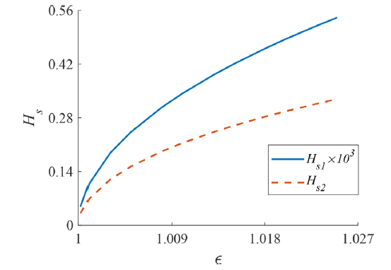
Fig. 3. The wave steepness of free surface Hs1 and internal interface Hs2 versus dimensionless angular frequency ϵ in the case of (86) when kh1=0.942 and kh2=12.566. |
Figure 4 shows the spatial profiles of free surface z=ζ1 and interface z=−h1+ζ2 with different dimensionless angular frequencies ϵ in one wave length. There is no doubt that increased ϵ leads to larger wave height. The wave height of internal interface is over 500 times larger than that of free surface for the case ϵ=1.025.

Fig. 4. The spatial profiles of (a) free surface z=ζ1(m) and (b) interface z=−h1+ζ2(m) at t=0(s) with dimensionless angular frequency ϵ in the case of (86) when kh1=0.942 and kh2=12.566. |
To determine the values of hydrodynamic coefficients CD and CM, the standard case kh1=0.942, kh2=12.566 and ϵ=1.025 with other parameters in (86) is selected here. For this case, the computed interfacial waves has the properties: wave steepness of the internal interface Hs2=0.329, wave height of the interface waves H2=105(m), maximum value of x− velocity component umax≈1.1(m/s), and wave period T=599(s). Since the kinematic viscosity of seawater ν≈10−6(m2/s), the Reynolds number Re=umaxD/ν≈5.5×106 and the Keulegan-Carpenter number Kc=πH2/D≈66. According to the experimental data in [27], the empirical coefficients are chosen as CD=0.6 and CM=1.8 for a smooth cylinder.
Figure 5 (a) displays the dependence on time t of the total drag and inertial forces estimated by the classical and modified Morison equations FD, FI, FI′ in one wave period. The curve of total drag force FD is symmetric about the minimum point, while the curves of total inertial forces FI and FI′ lack this symmetry. The peak value of FD is more than three times that of FI for the case kh1=0.942, kh2=12.566 and ϵ=1.025. The predicted value of inertial force peak of the modified Morison equation is slightly larger than that of the classical Morison equation in deep water for the case with strong nonlinearity.

Fig. 5. The total drag and inertial forces estimated by the classical and modified Morison equations FD(kN), FI(kN), FI′(kN) (a) and the global forces evaluated by the classical and modified Morison equations Fg(kN), Fg′(kN) (b) versus time t(s) in one wave period in the case of kh1=0.942, kh2=12.566 and ϵ=1.025, with other parameters in (86). |
Figure 5 (b) presents the global forces evaluated by the classical and modified Morison equations Fg and Fg′ versus time t in one wave period. The curves of the global forces estimated by the classical and modified Morison equations almost coincide with each other.
Figure 6 (a) provides the relationships between the maximum absolute values of forces (FD, FI, FI′, Fg and Fg′) and dimensionless angular frequency ϵ. All forces increase with ϵ, and it should be emphasized that the maximum absolute values of these two inertial forces both increase linearly with the dimensionless angular frequency. When the nonlinearity is small, the values of the drag force and these two global forces are all similar. The difference between the drag force and the global forces increases with nonlinearity, as well as the difference between the drag force and the inertial forces.
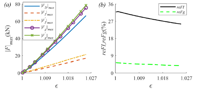
Fig. 6. The maximum absolute values of total drag and inertial forces |FD|max(kN), |FI|max(kN), |FI′|max(kN), and global forces |Fg|max(kN), |Fg′|max(kN) estimated by the classical and modified Morison equations (a) and the relative error between the total inertial forces and global forces reFI, reFg (b) versus dimensionless angular frequency ϵ in the case of kh1=0.942 and kh2=12.566, with other parameters in (86). |
Figure 6 (b) shows the relative errors between the total inertial forces and global forces reFI and reFg with various dimensionless angular frequencies ϵ. When the nonlinearity is weak, reFI is over 30%. As the nonlinearity increases, reFI decreases gradually. For strong nonlinearity, the value of reFI is still over 25%. The value of reFg remains small for different ϵ in the range of 3%∼6%. The difference between the inertial forces predicted by the classical and modified Morison equations cannot be neglected for interfacial periodic waves with any wave steepness in deep water.
3.2. Wave forces at various upper layer depths
Next, the influences of upper layer depth on interfacial waves and wave forces are computed and analysed in detail.
Figure 7 presents the relationship between wave steepness and upper layer depth parameter kh1. The wave steepness of free surface Hs1 first increases then decreases with kh1. The maximum value of Hs1 is at kh1=0.861. Similarly, the wave steepness of interface Hs2 increases first and then slowly decreases with kh1. The maximum value of Hs2 is at kh1=1.1. The free surface can be approximated as a rigid boundary for large water depth of upper layer, as shown in [17].
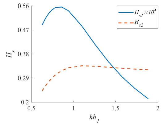
Fig. 7. The wave steepness of free surface Hs1 and internal interface Hs2 versus upper layer depth parameter kh1 in the case of (86) when ϵ=1.025 and kh2=12.566. |
Figure 8 shows the spatial profiles of free surface z=ζ1 and interface z=−h1+ζ2 with different upper layer depth parameters kh1 in one wave length. As the upper layer depth increases, the trough of surface waves becomes sharper while the crest of surface waves is almost unchanged. However, the corresponding crest and trough are both flattened with further growth of the upper layer depth. For interface waves, the crest is rather flat in the case kh1=0.628 due to the shallow upper water layer.
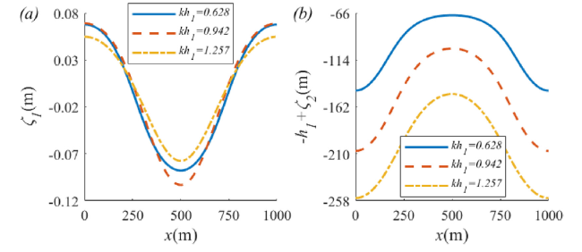
Fig. 8. The spatial profiles of (a) free surface z=ζ1(m) and (b) interface z=−h1+ζ2(m) at t=0(s) with upper layer depth parameter kh1 in the case of (86) when ϵ=1.025 and kh2=12.566. |
Figure 9 displays the dependence on time t of the total drag and inertial forces estimated by the classical and modified Morison equations FD, FI, FI′ for (a) and the dependence on time t of the global forces evaluated by the classical and modified Morison equations Fg and Fg′ for (b) in one wave period. Compared with Fig. 5, it is found that peaks of all wave forces decrease as the upper layer depth decreases from kh1=0.942 to kh1=0.628.
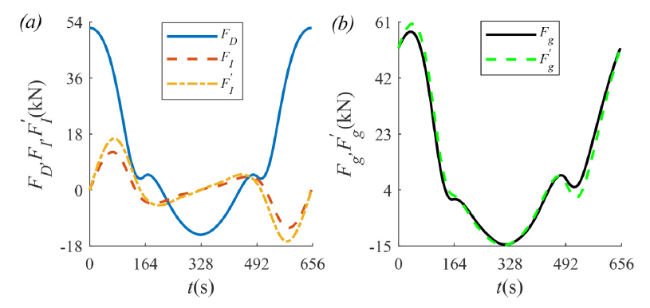
Fig. 9. The total drag and inertial forces estimated by the classical and modified Morison equations FD(kN), FI(kN), FI′(kN) (a) and the global forces evaluated by the classical and modified Morison equations Fg(kN), Fg′(kN) (b) versus time t(s) in one wave period in the case of kh1=0.628, kh2=12.566 and ϵ=1.025, with other parameters in (86). |
Figure 10 (a) provides the relationships between the maximum absolute values of forces (FD, FI, FI′, Fg and Fg′) and upper layer depth parameter kh1. FD, FI, FI′, Fg and Fg′ all first increase and then decrease with kh1, owning the same maximum point kh1=0.861 corresponding to that of Hs1. The estimated values of the global forces are both larger than that of the drag force for any given kh1. When the upper layer depth is small, the total drag force FD is far larger than the total inertial force FI or FI′. Nevertheless, the difference between total drag and inertial forces has decreased a lot when the upper layer depth is large.
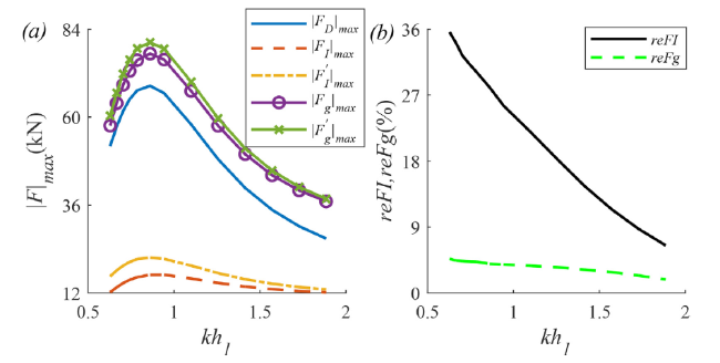
Fig. 10. The maximum absolute values of total drag and inertial forces |FD|max(kN), |FI|max(kN), |FI′|max(kN), and global forces |Fg|max(kN), |Fg′|max(kN) estimated by the classical and modified Morison equations (a) and the relative error between the total inertial forces and global forces reFI, reFg (b) versus upper layer depth parameter kh1 in the case of ϵ=1.025 and kh2=12.566, with other parameters in (86). |
Figure 10 (b) shows the relative errors between the total inertial forces and global forces reFI and reFg with various upper layer depth parameters kh1. reFI declines rapidly with kh1 from 35% to 6%. reFg remains below 5% for any upper layer depth. The difference between the inertial forces predicted by the classical and modified Morison equations is rather large for strongly nonlinear interfacial periodic waves with shallow upper fluid layer in deep water.
3.3. Wave forces at different lower layer depths
Finally, we focus on the cases with various lower layer depths from finite water depth to deep water.
Figure 11 presents the relationship between wave steepness and lower layer depth parameter kh2. As kh2 increases, the wave steepness of free surface and interface Hs1 and Hs2 both decrease rapidly when kh2<2.5, and then they stay almost the same in the range of kh2>3.1. The lower layer depth has obvious influence on the wave steepness of interfacial waves in finite water depth.
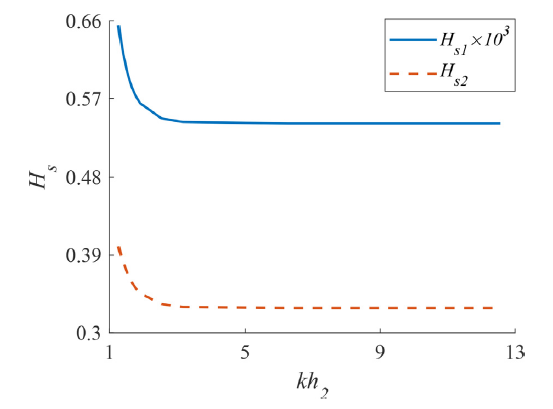
Fig. 11. The wave steepness of free surface Hs1 and internal interface Hs2 versus lower layer depth parameter kh2 in the case of (86) when ϵ=1.025 and kh1=0.942. |
Figure 12 shows the spatial profiles of free surface z=ζ1 and interface z=−h1+ζ2 with different lower layer depth parameters kh2 in one wave length. All crests and troughs decrease obviously with kh2 increasing from 1.257 to 2.513 while the shapes of free surface and interface are both nearly unchanged with kh2 further increasing from 2.513 to 12.566.
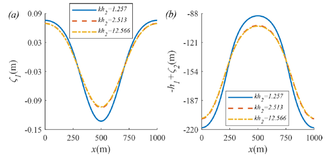
Fig. 12. The spatial profiles of (a) free surface z=ζ1(m) and (b) interface z=−h1+ζ2(m) at t=0(s) with lower layer depth parameter kh2 in the case of (86) when ϵ=1.025 and kh1=0.942. |
Figure 13 (a) displays the dependence on time t of the total drag and inertial forces estimated by the classical and modified Morison equations FD, FI, FI′ in one wave period. The symmetry of FD, and the asymmetry of FI and FI′ are the same as those in Fig. 5(a). Compared Fig. 13(a) with Fig. 5(a), the number of small fluctuations with time for all the three forces increases when the depth of lower water layer decreases. The predicted value of inertial force peak of the modified Morison equation is obviously larger than that of the classical Morison equation in finite water depth for strongly nonlinear cases.
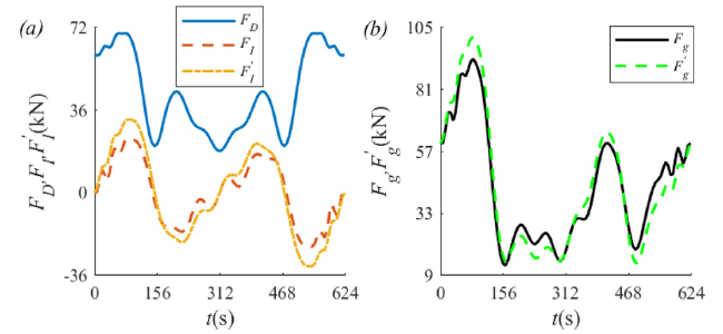
Fig. 13. The total drag and inertial forces estimated by the classical and modified Morison equations FD(kN), FI(kN), FI′(kN) (a) and the global forces evaluated by the classical and modified Morison equations Fg(kN), Fg′(kN) (b) versus time t(s) in one wave period in the case of kh1=0.942, kh2=1.257 and ϵ=1.025, with other parameters in (86). |
Figure 13 (b) presents the global forces evaluated by the classical and modified Morison equations Fg and Fg′ versus time t in one wave period. It is found that the difference between the global forces estimated by the classical and modified Morison equations decreases with the water depth by comparing Fig. 5(b) with Fig. 13(b).
Figure 14 (a) provides the relationships between the maximum absolute values of forces (FD, FI, FI′, Fg and Fg′) and lower layer depth parameter kh2. When kh2<3.1, FD first decreases and then increases with kh2; FI, FI′, Fg and Fg′ all decrease with kh2. However, these five forces are all nearly unchanged for the case kh2>3.1. The total drag force FD is more than twice the total inertial force FI or FI′ for any kh2. The variation of forces is concentrated in the cases with finite water depth.
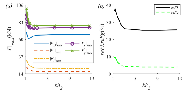
Fig. 14. The maximum absolute values of total drag and inertial forces |FD|max(kN), |FI|max(kN), |FI′|max(kN), and global forces |Fg|max(kN), |Fg′|max(kN) estimated by classical and modified Morison equations (a) and the relative error between the total inertial forces and global forces reFI, reFg (b) versus lower layer depth parameter kh2 in the case of ϵ=1.025 and kh1=0.942, with other parameters in (86). |
Figure 14 (b) shows the relative errors between the total inertial forces and global forces reFI and reFg with various lower layer depth parameters kh2. In the range of kh2<3.1, reFI first slightly rises to 38% at kh2=1.382 and then declines rapidly with kh2; reFg first slightly increases to 10% and then decreases with kh2. When kh2>3.1, the relative errors both change very little where the value of reFI is stable around 25% and the value of reFg is less than 4%. The difference between the inertial forces predicted by the classical and modified Morison equations is large for strongly nonlinear interfacial periodic waves in any water depth, and this relative error is particularly large for the case with shallow lower fluid layer in finite water depth. The difference between the global forces estimated via the classical and modified Morison equations can not be ignored when the lower layer depth is very small.
To sum up, every force evaluated by the modified Morison equation is inevitably larger than the corresponding force estimated via the classical Morison formula; the difference between the inertial forces predicted by the classical and modified Morison equations could be ignored only when the upper and lower layer depths are both large enough; the difference between the global forces estimated via the classical and modified Morison formulae could be neglected unless both the upper and lower layer depths are sufficiently small.
4. Concluding remarks
Series solutions of interfacial periodic gravity waves with a single primary component have been obtained in a two-layer fluid with free-surface boundary conditions. The physical parameters of fluid layers are chosen based on the real ocean enviroment. Both the classical and modified Morison equations are used to evaluate the forces on a cylindrical pile exerted by Boussinesq interfacial periodic waves. This paper extends the study of wave loads on a cylinder predicted by the modified Morison equation [12] from internal solitary wave loads to interfacial periodic wave loads.
The governing equations of fully nonlinear interfacial periodic waves with free surface are solved by the HAM. The solution procedure for the interfacial wave model with rigid upper boundary [17] has been developed to consider the free-surface boundary conditions. Convergent series solutions are obtained in the frame of the HAM.
For wave forces with increased nonlinearity, each inertial force peak increases linearly with the dimensionless angular frequency; the maximal inertial forces obtained by the modified Morison formulae is at least 25% larger than that obtained by the classical Morison formulae and this difference cannot be neglected for any wave steepness in deep water.
For wave forces with different upper layer depths, the maximum absolute values of total drag, inertial forces and global forces have the same maximum point at kh1=0.861, which is also the maximum point of the free surface steepness; the difference between the maximal inertial forces calculated by the classical and modified Morison equations is large (35% at kh1=0.628) for strongly nonlinear waves with thin upper fluid layer in deep water.
For wave forces with various lower layer depths, the difference between the maximal inertial forces predicted by the classical and modified Morison formulae stays above 25% for strongly nonlinear waves in any water depth, and this difference is rather large (38% at kh2=1.382) in finite water depth with thin lower fluid layer; the difference between the maximal global forces evaluated via the classical and modified Morison formulae reaches 10% and cannot be ignored for very small lower layer thickness in finite water depth. In addition, the number of small fluctuations for total drag and inertial forces in a wave period decreases with the lower layer depth.
To summarize, the results above indicate that the convective acceleration ignored in the classical Morison equation has significant influence on the riser’s inertial force caused by internal periodic waves, and this effect could be eliminated only in the case that the distance between the sea level and the density transition layer is sufficiently large in the deep sea. Therefore, for the prediction of internal periodic wave forces on marine risers in all shallow sea areas, the classical Morison equation is suggested to be replaced by the modified one.
In addition, Thorpe [26] pointed out that the free surface is equivalent to a rigid surface when the densities of these two fluid layers only have a small difference for a progressive interfacial wave system, which is the reason that the amplitude of the free surface is far smaller than that of the interface in this paper. Hence, wave profiles of the interface and related wave forces between rigid upper surface and free surface for the density ratio Δ=0.996 are similar. However, the free surface may have significant influences on other cases, such as interfacial waves with harmonic resonance [28], interfacial waves with triad resonance [29] and so on. Therefore, the HAM-based solution procedure in this manuscript for the interfacial wave model with free surface boundary conditions provides a way for future studies on interfacial wave resonances.
Declaration of Competing Interest
The authors declare that they have no known competing financial interests or personal relationships that could have appeared to influence the work reported in this paper.
Acknowledgments
This work was partly supported by the National Natural Science Foundation of China (Approval nos. 12202166, 12072126) and State Key Laboratory of Ocean Engineering (Shanghai Jiao Tong University) (Grant no. GKZD010087) in the study design, analysis and interpretation of data, writing of the report, and decision to submit the article for publication. This work was also partly supported by the Natural Science Foundation of Jiangsu Province, China (approval nos. BK20201006, BK20220652) in the collection of data.
Appendix A. Derivation of interface conditions
The two kinematic interface conditions at z=−h1+ζ2 are(A.1)∂ζ2∂t+∇ϕ1·∇ζ2−∂ϕ1∂z=0,and(A.2)∂ζ2∂t+∇ϕ2·∇ζ2−∂ϕ2∂z=0.The dynamic interface condition at z=−h1+ζ2 is(A.3)ρ1(∂ϕ1∂t+gζ2+12|∇ϕ1|2)−ρ2(∂ϕ2∂t+gζ2+12|∇ϕ2|2)=0.Given that Δ=ρ1/ρ2, the interface disturbance ζ2 is obtained by solving Eq. (A.3) to give at z=−h1+ζ2(A.4)ζ2=1g(1−Δ)[Δ(∂ϕ1∂t+12|∇ϕ1|2)−(∂ϕ2∂t+12|∇ϕ2|2)].
Carrying out partial differentiation of (A.4) with respect to x, y, and t, and substituting into Eqs. (A.1) and (A.2), ζ2 is then eliminated to give at z=−h1+ζ2(A.5)∂2ϕ2∂t2+g(1−Δ)∂ϕ2∂z−Δ∂2ϕ1∂t2+∂(|∇ϕ2|2)∂t−Δ∂(12|∇ϕ1|2)∂t+∇ϕ2·∇(12|∇ϕ2|2)−Δ∇ϕ2·∇(∂ϕ1∂t+12|∇ϕ1|2)=0,and(A.6)∂2ϕ2∂t2+g(1−Δ)∂ϕ1∂z−Δ∂2ϕ1∂t2+∂(12|∇ϕ2|2)∂t−Δ∂(|∇ϕ1|2)∂t−Δ∇ϕ1·∇(12|∇ϕ1|2)+∇ϕ1·∇(∂ϕ2∂t+12|∇ϕ2|2)=0.
Subtracting (A.6) from (A.5), we obtain at z=−h1+ζ2(A.7)g(1−Δ)∂(ϕ2−ϕ1)∂z+∂(12|∇ϕ2|2)∂t+∇ϕ2·∇(12|∇ϕ2|2)−∇ϕ1·∇(∂ϕ2∂t+12|∇ϕ2|2)+Δ[∂(12|∇ϕ1|2)∂t+∇ϕ1·∇(12|∇ϕ1|2)−∇ϕ2·∇(∂ϕ1∂t+12|∇ϕ1|2)]=0.
Subsequent derivation is then based on the kinematic interface conditions (A.5), (A.7) and dynamic interface condition (A.4). Note that Eq. (A.5) is (5), (A.7) is (6), and (A.4) is (7).
Appendix B. Expressions of high-order deformation equations in the HAM
Substituting the series (33) and (34) into the zeroth-order deformation Eqs. (28)-(32), and then equating like-powers of q, the following five linear equations (called high-order deformation equations) are obtained(B.1)L‾1[φm,1]=c0Δm−1,1φ+χm(Sm−1,1−S‾m,1),m≥1,(B.2)L‾i+1[φm,1,φm,2]=c0Δm−1,iφ+χm(Sm−1,i−S‾m,i),i=2,3,m≥1,(B.3)ηm,i=c0Δm−1,iη+χmηm−1,i,i=1,2,m≥1,where the auxiliary linear operators L‾1=L1|z=0, L‾3=L3|z=−h1, L‾4=L4|z=−h1, and(B.4)Δm,1φ=σ2ϕ¯m2,1,1+gϕ¯z,m0,1,1+Λm,11,1,1−2σΓm,11,1,(B.5)Δm,2φ=σ2ϕ¯m2,2,2+g(1−Δ)ϕ¯z,m0,2,2−Δσ2ϕ¯m2,1,2+Λm,12,2,2−2σΓm,12,2+Δ(σΓm,11,2−Λm,22,1,2−Λm,12,1,2),(B.6)Δm,3φ=g(1−Δ)(ϕ¯z,m0,2,2−ϕ¯z,m0,1,2)−σΓm,12,2+Λm,12,2,2−Λm,21,2,2−Λm,11,2,2+Δ(Λm,11,1,2−Λm,22,1,2−Λm,12,1,2−σΓm,11,2),(B.7)Δm,1η=ηm,1−1g(σϕ¯m1,1,1−Γm,01,1),(B.8)Δm,2η=ηm,2+1g(1−Δ)[Γm,02,2−σϕ¯m1,2,2+Δ(σϕ¯m1,1,2−Γm,01,2)],with the definition(B.9)Γm,0k‾,p=∑n=0m(k22ϕ¯n1,k‾,pϕ¯m−n1,k‾,p+12ϕ¯z,n0,k‾,pϕ¯z,m−n0,k‾,p),k‾,p=1,2,(B.10)Γm,1k‾,p=∑n=0m(k2ϕ¯n1,k‾,pϕ¯m−n2,k‾,p+ϕ¯z,n0,k‾,pϕ¯z,m−n1,k‾,p),k‾,p=1,2,(B.11)Γm,2k‾,p=∑n=0m(k2ϕ¯n1,k‾,pϕ¯z,m−n1,k‾,p+ϕ¯z,n0,k‾,pϕ¯zz,m−n0,k‾,p),k‾,p=1,2,(B.12)Λm,1i,j,p=∑n=0m(k2ϕ¯n1,i,pΓm−n,1j,p+ϕ¯z,n0,i,pΓm−n,2j,p),i,j,p=1,2,(B.13)Λm,2i,j,p=−σ∑n=0m(k2ϕ¯n1,i,pϕ¯m−n2,j,p+ϕ¯z,n0,i,pϕ¯z,m−n1,j,p),i,j,p=1,2,(B.14)μm,n,p={ηn,p,m=1,n≥1,∑i=m−1n−1μm−1,i,pηn−i,p,m≥2,n≥m,(B.15)ψi,k‾,1n,m=∂i∂ξi(1m!∂mφn,k‾∂zm|z=0),k‾=1,2,(B.16)ψi,k‾,2n,m=∂i∂ξi(1m!∂mφn,k‾∂zm|z=−h1),k‾=1,2,(B.17)βi,k‾,pn,m={ψi,k‾,pn,0,m=0,∑s=1mψi,k‾,pn,sμs,m,p,m≥1,(B.18)γi,k‾,pn,m={ψi,k‾,pn,1,m=0,∑s=1m(s+1)ψi,k‾,pn,s+1μs,m,p,m≥1,(B.19)δi,k‾,pn,m={2ψi,k‾,pn,2,m=0,∑s=1m(s+1)(s+2)ψi,k‾,pn,s+2μs,m,p,m≥1,(B.20)ϕ¯ni,k‾,p=∑m=0nβi,k‾,pn−m,m,ϕ¯z,ni,k‾,p=∑m=0nγi,k‾,pn−m,m,ϕ¯zz,ni,k‾,p=∑m=0nδi,k‾,pn−m,m.
Expressions for Li, Sm−1,i and S‾m,i, are given in Section 2.2.2.
