
1. Introduction
1.1. Aims, scope and origin of the problem
It is worth remembering that nonlinear partial differential equations (NPDEs) have stirred up researchers’ interest because NPDEs are used to govern a number of complex phenomena in applied and mathematical physics, which include ocean science [1], [2], [3], [4], heat flow in nano-fluids flows [5], [6], [7], [8], [9], [10], [11], [12], [13], [14], magnetohydrodynamics [15], [16], [17], [18], [19], [20], [21], plasma physics, fluid dynamics [22], [23], [24], [25], [26], [27], [28], [29], [30], [31], biomedical engineering [32], oceanography [33], [34], and cosmology etc.
In this research, analytical solutions of the following form of the system of (2+1)-coupled dispersive long wave equations (DLWEs) are obtained, which is governed by
$\begin{matrix} {} & {{u}_{yt}}+{{h}_{xx}}+{{u}_{x}}{{u}_{y}}+u{{u}_{xy}}=0, \\ {} & {{h}_{t}}+{{u}_{x}}+h{{u}_{x}}+u{{h}_{x}}+{{u}_{xxy}}=0. \\\end{matrix}$
One of the nonlinear evolution equations (NEEs) is the DLWE system. Inverse spectral transform (IST) in two spatial dimensions successfully solves NEEs [35]. The deviation height of the surface water wave transmitting along the x-axis is h in this system [35], with u being the horizontal wave velocity. System (1) represents dispersive water waves transmitting in an infinitely long channels with constant depth. These equations can be observed in open seas or in wide channels [36], [37].
Besides above, it is important to mention here that external and internal impulsive disturbances in an open ocean causes a wave motion. In such a motion, a water column from bottom to water surface propagates in the direction of wave motion. These waves are the result of interaction between resonance and shearing forces which occur in oceans due to the action of wind in water. Its impact can be observed on the water surface [4]. Such surface waves usually have a very longer wavelength than that of the depth of the propagating ocean basis. One can call them as long water waves. If depth-averaged approximations [33] of Navier-Stokes equation (NSEs) is performed, then NSEs are termed as shallow water wave equations (SWWEs). Long water waves are an approximation of the Boussinesq type and such equations are stable with respect to short perturbations [38]. The long water wave travels faster in the deep water. Gravity waves have a faster phase speed in deeper water than they do in shallower water. Such waves usually have differences in heights, wave lengths and time durations advancing in different directions [35].
These equations satisfy Lax pair compatibility condition [40]
[T1,T2]≡0 between two operators viz. principle spectral operator, T1 and auxiliary spectral operator, T2. The operator T1 involves only spatial variables in coefficients function and T2 gives evolution of spectral transform of the potential functions [35].
It is imperative to mention that the Lax pair condition [T1,T2]≡0 is compatible only for trivial NEEs [41]. This difficulty is resolved [35] by compatibility condition $\left[ {{T}_{1}},{{T}_{2}} \right]L\left( x,y,t \right)\equiv 0$, where L is a tempo-spatial functional and operators T1 and T2 commute on the functional subspace L(x, y, t). For a function ϕ, the pair of equations $\left[ {{T}_{1}},{{T}_{2}} \right]\phi =0$ and ${{T}_{1}}\phi =0$ yields Eq. (1), when substitutions are taken as u=2R and $h=-1-4Q+2{{R}_{y}}$, Q, R are potential functions [35].
$\begin{matrix} {} & {{u}_{t}}+g{{h}_{x}}+u{{u}_{x}}=0, \\ {} & {{h}_{t}}+{{u}_{x}}{{H}_{avg}}+H_{avg}^{\prime }u+{{u}_{x}}h+u{{h}_{x}}=0, \\\end{matrix}$
where u(x, t) is the zonal velocity, h(x, t) represents the height deviation or surface elevation, ${{H}_{avg}}\left( x \right)$ is the sea depth near the coast and g is the gravitational acceleration. Prime on ${{H}_{avg}}$ denotes its derivative [34].
The term dispersion of wave refers to the phenomenon of frequency dispersion, in which waves of different wavelengths travel at varying phase speeds on the free water surface, with gravity and surface tension acting as restoring forces.
Moreover, in dispersion long wave travels faster than shorter ones. If the depth of water <$\frac{1}{20}$ of the wavelength of wave, the wave is long gravity wave, and its wavelength is directly proportional to its periodic time.
1.2. Literature review
To get the exact solutions of a system of NPDEs is not an easy task. Considering different issues in different methods/tools, a good number of researches [38], [39], [40], [41], [42], [43], [44], [45], [46], [47], [48], [49], [50], [51], [52], [53], [54], [55], [56], [57], [58], [59], [60], [61], [62], [63], [64], [65], [66], [67], [68] are listed in Table 1 citing analytical and some particular solutions of the test system (1). The table provides exclusive information about the nature of these solutions which are obtained by using some techniques/tools notably Hamiltonian theory [38], inverse spectral transform [35], expansion method [39], extended mapping transformations [42], [43], generalized direct [44], direct method and non-classical Lie group theory [45], extended tanh method [46], extended mapping [47], tanh method [48], Lie point symmetries with Kac-Moody-Virasoro symmetry algebra [49], homogeneous balance method [50], [51], [52], Clarkson-Kruskal direct and similarity reduction [45], [53], [54], [55], [56], standard Painlevé truncation [57], Painlevé Bäcklund transformation and simplified Hirota method [58], Bäcklund transformation [59], Hirota bilinear [60], [61], F-expansion and balance method [62], [63], Mapping approach via Riccati equation [64], [65], optimal subalgebra [36], [37], generalized symmetries and algebra [66], singular manifold [67] and successive approximation method [68]. Furthermore, Kumar et al. [36] and Sharma et al. [37] generated optimal classes of subalgebra for system (1) and found some solitons and exact solutions.
Table 1. Different types of solutions derived for system of DLWEs. |
| Author | Method | Solutions |
|---|---|---|
| Boiti et al. [35] | Inverse spectral transform | Soliton-like |
| Kumar et al. [36], | Optimal subalgebra | Soliton, |
| Sharma et al. [37], | ” | Exact |
| Broer [38] | Hamiltonian theory | Wave travelling |
| Lou [39] | Expansion | Lumps, movable singularity manifold |
| Bai and Zhao [42], | Extended mapping transformation | Dromion, ring, foldon, peakon |
| Bai and Niu [43] | ” | compacton; quasi-periodic |
| non-periodic | ||
| Dong and Chen [44] | Generalized Direct | Oscillated dromions, soliton |
| Lou [45] | Direct method & non-classical | Trivial |
| Lie group theory | ||
| Zhi et al. [46] | Further extended tanh | Soliton, Periodic, rational |
| Fang et al. [47] | Extended mapping | Dromion, ring, peakon, compacton |
| Wang et al. [48] | tanh | Soliton, rational, periodic |
| Zhang et al. [49] | Lie point symmetries Kac-Moody- | DLWEs Eq. is reduced only |
| Virasoro symmetry algebra | ||
| Zhang and Niu [50], | Homogeneous balance | Multisoliton, solitary wave |
| Wang et al. [51], | ” | Dromions, lumps, breathers |
| Zhang and Chen [52] | instantons, ring solitons | |
| Tang et al. [53], | Clarkson-Kruskal direct | Periodic, chaotic |
| Tian et al. [54], | & similarity reduction | soliton-like |
| Liu et al. [55], | ” | dromion |
| Ma et al. [56] | ” | explicit reduction |
| Tang et al. [57], | Standard Painlevé truncation | Ring, soliton, chaotic, |
| fractal, dromions | ||
| Wazwaz [58] | Painlevé Bäcklund transformation, | Multiple solitons |
| simplified Hirota method | ||
| Wen [59], | Backlund transformation | Dromions compactons, peakons |
| Xue et al. [60], | Hirota bilinear | m- soliton, travelling wave, one-, |
| Ma [61] | “ | two-, three- and N-soliton, dromion |
| Tian et al. [62], [63] | F-expansion & balance | Periodic wave, solitary wave, |
| triangular periodic, wave | ||
| Ma et al. [64], | Mapping approach via Riccati Eq. | Multiple-soliton, Weierstrass function |
| Ma and Hu [65] | “ | periodic soliton, |
| Lou [66] | Generalized symmetries & algebra | Non-trivial |
| Peng and Krishnan [67] | Singular manifold | Periodic & solitary waves, |
| dromion, solitoff-like | ||
| Manaa et al. [68] | Successive approximation | Solitary waves |
1.3. Motivation and objective
Being motivated by the above researches, the authors derived some new solutions using similarity transformations method (STM) via one-parameter Lie group theory. The Lie group theory or Lie-symmetry analysis was developed by Sophus Lie in 1881 to integrate the partial and ordinary differential equations (ODE) analytically. The STM enables to reduce the number of independent variables in a system of PDEs with or without boundary conditions. Obviously, repeated use of the STM can transform or reduce the system of PDEs into system of ODEs. In case of ODE, if STM is employed then order of ODE is reduced by one in once reduction. In each similarity reduction, the system of differential equations remains unchanged, this phenomenon is called invariance. Invariance condition for the system of PDEs along with use of PDEs, can provide an over-determining system of new PDEs involving infinitesimal generators which are the functions of independent variables and dependent variables and such transformations give similarity variables and similarity functions with the help of Lagrange’s equations. Similarity variables are the new variables connecting original variables to produce one less number of variables. Similarity functions are able to produce similar forms of the solutions. As a result, the STM is a useful tool for obtaining analytical solutions to nonlinear/linear PDEs and ODEs. One can go through the rich literature Kumar et al. [36], Sharma et al. [37], Lou [66], Peng and Krishnan [67], Manaa et al. [68], Novikov et al. [41], Lax [40], Paquin and Winternitz [69], Kumar and Rani [70], Kumar et al. [71], Kumar and Kumar [72], Kumar et al. [73], Kumar and Tiwari [74], Kumar and Tiwari [75], Kumar [76], Kumar et al. [77], Kumar and Kumar [78] and references therein for the description of the STM and applications.
This article is structured as follows: In the next section, invariant solutions are obtained using Lie symmetry analysis. Physical analysis of solutions is discussed in Section 3. This section includes comparison of results derived in this article with the previous findings [36], [37]. The last section of the paper contains concluding remarks.
2. Similarity transformations method and invariant solutions
This section provides a basic overview of the STM using one-parameter Lie group theory. Because in a system of PDEs, the STM reduces the number of independent variables by one, it can be used repeatedly to convert the system of PDEs into an ODE system. In each similarity reduction process, the system of PDEs (1) remains unchanged. The invariance criteria produces an over-determining system of PDEs with infinitesimal generators satisfying the system of PDEs (1). Infinitesimals are helpful to get similarity variables and similarity functions. The number of independent variables in the test system (1) is reduced by one using these variables.
Introducing the required derivatives of the dependent variables into the system (1), it generates a new reduced system of PDEs, which may then be used repeatedly to generate a new system of ODEs. Ultimately, a solution of such ODEs after using back substitution gives an analytical solution of the system of PDEs (1). To achieve the analytical solutions of the system (1), Let us take the one-parameter (ϵ) Lie-group of transformations as:
$\begin{array}{l} x^{*}=\chi+\epsilon \xi^{(1)}(\chi)+O\left(\epsilon^{2}\right) \\ y^{*}=y+\epsilon \xi^{(2)}(\chi)+O\left(\epsilon^{2}\right) \\ t^{*}=t+\epsilon \tau(\chi)+O\left(\epsilon^{2}\right) \\ u^{*}=u+\epsilon \eta^{(1)}(\chi)+O\left(\epsilon^{2}\right) \\ h^{*}=h+\epsilon \eta^{(2)}(\chi)+O\left(\epsilon^{2}\right) \end{array}$
where ξ(1),ξ(2), τ, ηu and ${{\eta }_{h}}$ are the infinitesimals for the variables x, y, t, u and h respectively. Notation (χ) denotes (x, y, t, u, h) and star equipped with superscript of a variable denotes the value of the variable in transformed space. Basic characteristics of the similarity transformations is invariance, i.e. a derivative remains unaltered after employing the transformations [71], [73], [75], [77], [79], [80].
The vector field V be corresponding to the transformations, and can be written as:
$V={{\xi }^{\left( 1 \right)}}\frac{\partial }{\partial x}+{{\xi }^{\left( 2 \right)}}\frac{\partial }{\partial y}+\tau \frac{\partial }{\partial t}+{{\eta }^{\left( 1 \right)}}\frac{\partial }{\partial u}+{{\eta }^{\left( 2 \right)}}\frac{\partial }{\partial h}.$
$\begin{aligned} \operatorname{Pr}^{(2)} V= & V+\left[\eta_{x}^{(1)}\right] \frac{\partial}{\partial\left(u_{x}\right)}+\left[\eta_{y}^{(1)}\right] \frac{\partial}{\partial\left(u_{y}\right)}+\left[\eta_{y t}^{(1)}\right] \frac{\partial}{\partial\left(u_{y t}\right)} \\ & +\left[\eta_{x x}^{(2)}\right] \frac{\partial}{\partial\left(h_{x x}\right)}+\left[\eta_{x y}^{(1)}\right] \frac{\partial}{\partial\left(u_{x y}\right)} \end{aligned}$,
$\begin{aligned} \operatorname{Pr}^{(3)} V= & V+\left[\eta_{t}^{(2)}\right] \frac{\partial}{\partial\left(h_{t}\right)}+\left[\eta_{x}^{(1)}\right] \frac{\partial}{\partial\left(u_{x}\right)} \\ & +\left[\eta_{x}^{(2)}\right] \frac{\partial}{\partial\left(h_{x}\right)}+\left[\eta_{x x y}^{(1)}\right] \frac{\partial}{\partial\left(u_{x x y}\right)} \end{aligned}$,
where extensions of different orders like $\left[ \eta _{x}^{\left( 1 \right)} \right]$, $\left[ \eta _{y}^{\left( 1 \right)} \right]$, $\left[ \eta _{t}^{\left( 2 \right)} \right],$ $\left[ \eta _{xx}^{\left( 2 \right)} \right]$,$\left[ \eta _{xy}^{\left( 1 \right)} \right]$, $\left[ \eta _{yt}^{\left( 1 \right)} \right]$, and $\left[ \eta _{xxy}^{\left( 1 \right)} \right]$ can be referred from Bluman and Cole [79], Olver [80].
The invariance condition for the system (1) can be written as:
$\begin{matrix} {} & P{{r}^{\left( 2 \right)}}V\left[ {{u}_{yt}}+{{h}_{xx}}+{{u}_{x}}{{u}_{y}}+u{{u}_{xy}} \right]=0, \\ {} & P{{r}^{\left( 3 \right)}}V\left[ {{h}_{t}}+{{u}_{x}}+h{{u}_{x}}+u{{h}_{x}}+{{u}_{xxy}} \right]=0. \\\end{matrix}$
It recasts as:
$\begin{matrix} {} & \left[ \eta _{yt}^{\left( 1 \right)} \right]+\left[ \eta _{xx}^{\left( 2 \right)} \right]+{{\theta }_{y}}\left[ \eta _{x}^{\left( 1 \right)} \right]+{{\theta }_{x}}\left[ \eta _{y}^{\left( 1 \right)} \right]+{{\theta }_{xy}}{{\eta }^{\left( 1 \right)}}+u\left[ \eta _{xy}^{\left( 1 \right)} \right]=0, \\ {} & \left[ \eta _{t}^{\left( 2 \right)} \right]+\left( h+1 \right)\left[ \eta _{x}^{\left( 1 \right)} \right]+{{\theta }_{x}}{{\eta }^{\left( 2 \right)}}+{{\phi }_{x}}{{\eta }^{\left( 1 \right)}}+u\left[ \eta _{x}^{\left( 2 \right)} \right]+\left[ \eta _{xxy}^{\left( 1 \right)} \right]=0. \\ \end{matrix}$
Making use of the system (1) into invariant conditions represented by (8) and solving them, the following overdetermined system of PDEs can be obtained
$\begin{array}{l} \xi_{y}^{(1)}=\xi_{u}^{(1)}=\xi_{h}^{(1)}=\xi_{x}^{(2)}=\xi_{u}^{(2)}=\xi_{h}^{(2)}=0 \\ \tau_{x}=\tau_{y}=\tau_{u}=\tau_{h}=0 \\ \xi_{x}^{(1)}=\frac{1}{2} \tau_{t}, \eta^{(1)}=\xi_{t}^{(1)}-\frac{u}{2} \tau_{t} \\ \eta^{(2)}=-(1+h)\left(\frac{1}{2} \tau_{t}+\xi_{y}^{(2)}\right) \end{array}$
After solving it, the following infinitesimals of the system (1) can be obtained:
$\begin{array}{l} \xi^{(1)}=\frac{1}{2} x f_{1}^{\prime}(t)+f_{3}(t), \xi^{(2)}=f_{2}(y), \tau=f_{1}(t) \\ \eta^{(1)}=\frac{1}{2} x f_{1}^{\prime \prime}(t)+f_{3}^{\prime}(t)-\frac{1}{2} u f_{1}^{\prime}(t) \\ \eta^{(2)}=-\left(\frac{1+h}{2}\right)\left(2 f_{2}^{\prime}(y)+f_{1}^{\prime}(t)\right) \end{array} $
where prime denotes the derivative of fi’s, 1≤i≤3. f1, f3 are regular functions of temporal variable t, while f2(y) involves only space variable.
In this work, infinitesimals of the system (1) are same as found in Kumar et al. [36] and Sharma et al. [37], but here, authors found the analytical solutions without choosing particular forms of ${{f}_{1}}\left( t \right)$ and ${{f}_{2}}\left( y \right)$ as done in Kumar et al. [36] and Sharma et al. [37] to generate optimal classes of subalgebra for the system (1). It is well-known fact that different choices of such functions can generate many similarity reductions. In this research, all invariant solutions are derived without taking particular forms of ${{f}_{1}}\left( t \right)$, ${{f}_{2}}\left( y \right)$ while ${{f}_{3}}\left( t \right)$ is taken as $\frac{{{a}_{0}}}{2}f_{1}^{\prime }\left( t \right)$(a0 being a constant).
Now, generator of Lie algebra is given by
$v={{v}_{1}}\left( {{f}_{1}} \right)+{{v}_{2}}\left( {{f}_{2}} \right)+{{v}_{3}}\left( {{f}_{3}} \right),$, where vi’s, i=1, 2, 3 can be represented as
$\begin{matrix} {{v}_{1}}\left( {{f}_{1}} \right) & =\frac{x}{2}f_{1}^{\prime }\left( t \right)\frac{\partial }{\partial x}+{{f}_{1}}\left( t \right)\frac{\partial }{\partial t}+\frac{1}{2}\left( xf_{1}^{\prime\prime }\left( t \right)-uf_{1}^{\prime }\left( t \right) \right)\frac{\partial }{\partial u} \\ {} & -\frac{1}{2}\left( 1+h \right)f_{1}^{\prime }\left( t \right)\frac{\partial }{\partial h}, \\ {{v}_{2}}\left( {{f}_{2}} \right) & ={{f}_{2}}\left( y \right)\frac{\partial }{\partial y}-\left( 1+h \right)f_{2}^{\prime }\left( y \right)\frac{\partial }{\partial h}, \\ {{v}_{3}}\left( {{f}_{3}} \right) & ={{f}_{3}}\left( t \right)\frac{\partial }{\partial x}+f_{3}^{\prime }\left( t \right)\frac{\partial }{\partial u}. \\ \end{matrix}$
Following commutator table (Table 2) shows the complete information of the Lie group ().
Table 2. Commutator table for (1). |
| v1 | v2 | v3 | |
|---|---|---|---|
| v1 | 0 | 0 | $v_{3}\left(f_{1} f_{3}^{\prime}-\frac{1}{2} f_{3} f_{1}^{\prime}\right) $ |
| v2 | 0 | 0 | 0 |
| v3 | $-v_{3}\left(f_{1} f_{3}^{\prime}-\frac{1}{2} f_{3} f_{1}^{\prime}\right)$ | 0 | 0 |
Therefore, the above discussion provides the following characteristic equation by means of Lagrange for the system of Eq. (1) as:
$\begin{matrix} {} & \frac{2dx}{xf_{1}^{\prime }\left( t \right)+2{{f}_{3}}\left( t \right)}=\frac{dy}{{{f}_{2}}\left( y \right)}=\frac{dt}{{{f}_{1}}\left( t \right)} \\ {} & =\frac{2du}{xf_{1}^{\prime\prime }\left( t \right)+2f_{3}^{\prime }\left( t \right)-uf_{1}^{\prime }\left( t \right)}=-\frac{2dh}{\left( 1+h \right)\left( 2f_{2}^{\prime }\left( y \right)+f_{1}^{\prime }\left( t \right) \right)}. \\ \end{matrix}$
To proceed the further integration, we have restricted ${{f}_{3}}\left( t \right)=\frac{{{a}_{0}}}{2}f_{1}^{\prime }\left( t \right)$, which follows the similarity reduction as:
$\begin{matrix} u & =\frac{\left( x+{{a}_{0}} \right)}{2}\frac{f_{1}^{\prime }\left( t \right)}{{{f}_{1}}\left( t \right)}+\frac{U\left( X,Y \right)}{\sqrt{{{f}_{1}}\left( t \right)}}, \\ {} & h=\frac{H\left( X,Y \right)}{{{f}_{2}}\left( y \right)\sqrt{{{f}_{1}}\left( t \right)}}-1,{{f}_{2}}\left( y \right)\ne 0 \\ \end{matrix}$
where $X=\frac{x+{{a}_{0}}}{\sqrt{{{f}_{1}}\left( t \right)}},{{f}_{1}}\left( t \right)\ne 0$, and $Y=\int \frac{1}{{{f}_{2}}\left( y \right)}dy-\int \frac{1}{{{f}_{1}}\left( t \right)}dt$.
The derivatives of the values are as follows:
$\begin{array}{l} u_{x}=\frac{f_{1}^{\prime}}{2 f_{1}(t)}+\frac{U_{X}}{f_{1}(t)}, u_{y}=\frac{U_{Y}}{\left(f_{1}(t)\right)^{\frac{1}{2}} f_{2}(y)} \\ u_{t y}=-\frac{1}{f_{2}(y)}\left[\frac{U_{Y} f_{1}^{\prime}}{2\left(f_{1}\right)^{\frac{3}{2}}}+\frac{X U_{X Y} f_{1}^{\prime}}{2\left(f_{1}\right)^{\frac{3}{2}}}+\frac{U_{Y Y}}{\left(f_{1}\right)^{\frac{3}{2}}}\right] \\ u_{x x y}=\frac{U_{X X Y}}{\left(f_{1}\right)^{\frac{3}{2}} f_{2}(y)}, h_{x}=\frac{H_{X}}{f_{2}(y)\left(f_{1}(t)\right)} \\ h_{t}=-\frac{1}{f_{2}(y)}\left[\frac{H f_{1}^{\prime}}{2\left(f_{1}\right)^{\frac{3}{2}}}+\frac{X H_{X} f_{1}^{\prime}}{2\left(f_{1}\right)^{\frac{3}{2}}}+\frac{H_{Y}}{\left(f_{1}\right)^{\frac{3}{2}}}\right] \text { etc. } \end{array}$
Inserting the values of the derivatives, the first similarity reduction of the DLWEs (1) provides
$\begin{matrix} {} & -{{U}_{YY}}+{{H}_{XX}}+{{U}_{X}}{{U}_{Y}}+U{{U}_{XY}}=0, \\ {} & -{{H}_{Y}}+H{{U}_{X}}+U{{H}_{X}}+{{U}_{XXY}}=0. \\\end{matrix}$
The infinitesimals for it, are as follows:
$\begin{matrix} {} & {{\xi }_{X}}={{a}_{1}}+{{a}_{2}}X,{{\xi }_{Y}}={{a}_{3}}+2{{a}_{2}}Y, \\ {} & {{\eta }_{U}}=-{{a}_{2}}U,{{\eta }_{H}}=-3{{a}_{2}}H, \\\end{matrix}$
where ai’s, 1≤i≤3 are arbitrary constants.
Therefore, generator of finite dimensional Lie-algebra is given by$W={{a}_{1}}{{W}_{1}}+{{a}_{2}}{{W}_{2}}+{{a}_{3}}{{W}_{3}}$ where
${{W}_{1}}=\frac{\partial }{\partial X},{{W}_{2}}=X\frac{\partial }{\partial X}+2Y\frac{\partial }{\partial Y}-U\frac{\partial }{\partial U}-3H\frac{\partial }{\partial H},{{W}_{3}}=\frac{\partial }{\partial Y}.$
Table 3. Commutator table for (14). |
| W1 | W2 | W3 | |
|---|---|---|---|
| W1 | 0 | W1 | 0 |
| W2 | - W1 | 0 | -2 W3 |
| W3 | 0 | 2 W3 | 0 |
Table 4. Adjoint table for (14). |
| Ad | W1 | W2 | W3 |
|---|---|---|---|
| W1 | W1 | $W_{2}-\epsilon W_{1}$ | W33 |
| W2 | $W_{1} e^{\epsilon}$ | W2 | $W_{3} e^{2 \epsilon}$ |
| W3 | W1 | $W_{2}-2 \epsilon W_{3}$ | W3 |
The corresponding Lagrange’s system for the first reduction (14) is
$\frac{dX}{{{a}_{1}}+{{a}_{2}}X}=\frac{dY}{{{a}_{3}}+2{{a}_{2}}Y}=-\frac{dU}{{{a}_{2}}U}=-\frac{dH}{3{{a}_{2}}H},$
To proceed further, following cases can be raised:
Case (I): If a2≠0, then Eq. (15) recasts as
$\frac{dX}{{{A}_{1}}+X}=\frac{dY}{{{A}_{2}}+2Y}=-\frac{dU}{U}=-\frac{dH}{3H}.$
Thus, for further similarity reduction, the similarity variable and similarity functions are
${{X}_{1}}=\frac{{{A}_{1}}+X}{\sqrt{{{A}_{2}}+2Y}},\ U=\frac{F\left( {{X}_{1}} \right)}{\sqrt{{{A}_{2}}+2Y}},H=\frac{G\left( {{X}_{1}} \right)}{{{\left( {{A}_{2}}+2Y \right)}^{\frac{3}{2}}}},$
where ${{A}_{1}}=\frac{{{a}_{1}}}{{{a}_{2}}}$ and ${{A}_{2}}=\frac{{{a}_{3}}}{{{a}_{2}}}$.
Therefore, the corresponding reduction of the system (14) yields
$3F+5{{X}_{1}}{F}'+X_{1}^{2}{F}''-{G}''+3F{F}'+{{X}_{1}}{{\left( {{F}'} \right)}^{2}}+{{X}_{1}}F{F}''=0,$
$3 G+X_{1} G^{\prime}+G F^{\prime}+F G^{\prime}-3 F^{\prime \prime}-X_{1} F^{\prime \prime \prime}=0$
To solve it further, we have split the family of solutions in the following sub cases:
Case (Ia): Taking $F=-\frac{3}{2}{{X}_{1}}$, $G=-\frac{1}{2}X_{1}^{3}$
The solution of DLWEs can be read as:
${{u}_{1}}=\frac{\left( x+{{a}_{0}} \right)}{2}\frac{f_{1}^{\prime }\left( t \right)}{{{f}_{1}}\left( t \right)}-\frac{3}{2}\frac{\left( {{A}_{1}}+X \right)}{\left( {{A}_{2}}+2Y \right)\sqrt{{{f}_{1}}\left( t \right)}},$
$h_{2}=\frac{C_{1}\left(A_{1}+X\right)}{\left(A_{2}+2 Y\right)^{2} f_{2}(y) \sqrt{f_{1}(t)}}-1 $
Case (Ib): Assuming F=−2X1, $G={{C}_{1}}X_{1}^{3}$, (where C1 being arbitrary constant). Then the solution of system of DLWEs (1) can be obtained as
${{u}_{2}}=\frac{\left( x+{{a}_{0}} \right)}{2}\frac{f_{1}^{\prime }\left( t \right)}{{{f}_{1}}\left( t \right)}-\frac{2\left( {{A}_{1}}+X \right)}{\left( {{A}_{2}}+2Y \right)\sqrt{{{f}_{1}}\left( t \right)}},$
$h_{2}=\frac{C_{1}\left(A_{1}+X\right)}{\left(A_{2}+2 Y\right)^{2} f_{2}(y) \sqrt{f_{1}(t)}}-1 $
Case (Ic): By setting $F=-2{{X}_{1}}+\frac{{{C}_{2}}}{{{X}_{1}}}$, $G={{C}_{3}}{{X}_{1}}$, (where C2, C3 are arbitrary constants).
Then solution is
${{u}_{3}}=\frac{\left( x+{{a}_{0}} \right)}{2}\frac{f_{1}^{\prime }\left( t \right)}{{{f}_{1}}\left( t \right)}+\frac{1}{\sqrt{{{f}_{1}}\left( t \right)}}\left[ \frac{{{C}_{2}}}{{{A}_{1}}+X}-\frac{2\left( {{A}_{1}}+X \right)}{{{A}_{2}}+2Y} \right],$
$h_{3}=\frac{C_{3}\left(A_{1}+X\right)}{\left(A_{2}+2 Y\right)^{2} f_{2}(y) \sqrt{f_{1}(t)}}-1 $
Case (II): Taking ${{a}_{2}}=0,{{a}_{3}}\ne 0$ in Eq. (17), Lagrange’s characteristic equation gives
$\frac{dX}{{{a}_{1}}}=\frac{dY}{{{a}_{3}}}=\frac{dU}{0}=\frac{dV}{0}.$
Then, similarity variable and similarity functions are
${{X}_{2}}=X-{{A}_{4}}Y,$ where ${{A}_{4}}=\frac{{{a}_{1}}}{{{a}_{3}}}$
$U=F\left(X_{2}\right), V=G\left(X_{2}\right) $
Then reduced form of the Eq. (14) is given by
$A_{4}^{2}{F}'\text{ }\!\!'\!\!\text{ }-{G}'\text{ }\!\!'\!\!\text{ }+{{A}_{4}}{{\left( {{F}'} \right)}^{2}}+{{A}_{4}}F{F}'\text{ }\!\!'\!\!\text{ }=0,$
$A_{4} G^{\prime}+G F^{\prime}+F G^{\prime}-A_{4} F^{\prime \prime \prime}=0$
Intigration of Eq. (29) gives
$G=\frac{{{C}_{4}}+{{A}_{4}}{F}''}{F+{{A}_{4}}}.$
where C4 is an arbitrary constant of integration
Twice integration of Eq. (28) gives
$-A_{4}^{2}F+G-\frac{{{A}_{4}}}{2}{{F}^{2}}={{C}_{5}}{{X}_{2}}+{{C}_{6}}.$
C5 and C6 are arbitrary constants.
Putting the value of G from Eq. (30) in Eq. (31), One can get
$\begin{matrix} {} & {{A}_{4}}{F}''-\frac{{{A}_{4}}}{2}{{F}^{3}}-\frac{3}{2}A_{4}^{2}{{F}^{2}}-F\left( A_{4}^{3}+{{C}_{5}}{{X}_{2}}+{{C}_{6}} \right) \\ {} & \quad +\left( {{C}_{4}}-{{C}_{5}}{{A}_{4}}{{X}_{2}}-{{C}_{6}}{{A}_{4}} \right)=0. \\\end{matrix}$
Restricting C5 = 0 and integrating, authors get
${{\left( {{F}'} \right)}^{2}}-\frac{1}{4}{{F}^{4}}-{{A}_{4}}{{F}^{3}}-\left( \frac{{{C}_{6}}}{{{A}_{4}}}+A_{4}^{2} \right){{F}^{2}}-\left( 2{{C}_{6}}-2\frac{{{C}_{4}}}{{{A}_{4}}} \right)F={{C}_{7}}.$
Case (IIa): By setting ${{A}_{4}}=-{{k}_{1}}$, ${{C}_{4}}=\frac{3}{2}k_{1}^{4}$, ${{C}_{6}}=-k_{1}^{3}$, ${{C}_{7}}=\frac{1}{4}k_{1}^{4}$ in Eq. (33). Then solutions are
${{u}_{4}}=\frac{\left( x+{{a}_{0}} \right)}{2}\frac{f_{1}^{\prime }\left( t \right)}{{{f}_{1}}\left( t \right)}+\frac{1}{\sqrt{{{f}_{1}}\left( t \right)}}\left[ {{k}_{1}}-\frac{2}{{{C}_{8}}\pm \left( X+{{k}_{1}}Y \right)} \right],$
$h_{4}=\frac{1}{f_{2}(y) \sqrt{f_{1}(t)}}\left[\frac{-2 k_{1}}{\left\{C_{8} \pm\left(X+k_{1} Y\right)\right\}^{2}}-\frac{k_{1}^{3}}{2}\right]-1$.
Case (IIb): Treating A4≠0, C4=C6=C7=0 in Eq. (33), the solution of system DLWEs. (1) can be furnished as
$\begin{matrix} {{u}_{5}} & =\frac{\left( x+{{a}_{0}} \right)}{2}\frac{f_{1}^{\prime }\left( t \right)}{{{f}_{1}}\left( t \right)}+\frac{1}{\sqrt{{{f}_{1}}\left( t \right)}}\times \\ {} & \left[ \frac{2{{A}_{4}}{{C}_{9}}\exp \left( \pm {{A}_{4}}\left( X-{{A}_{4}}Y \right) \right)}{1-{{C}_{9}}\exp \left( \pm {{A}_{4}}\left( X-{{A}_{4}}Y \right) \right)} \right], \\ \end{matrix}$
$h_{5}=\frac{1}{f_{2}(y) \sqrt{f_{1}(t)}}\left[\frac{2 A_{4}^{3} C_{9} \exp \left( \pm A_{4}\left(X-A_{4} Y\right)\right)}{\left\{1-C_{9} \exp \left( \pm A_{4}\left(X-A_{4} Y\right)\right)\right\}^{2}}\right]-1$
Case (IIc): By assuming ${{A}_{4}}=-{{a}^{2}}$, ${{C}_{4}}=-{{a}^{2}}\left( 1+{{a}^{6}} \right)$, ${{C}_{6}}=1+{{a}^{6}}$, C7=0 in Eq. (33), the solution of DLWEs (1) yields
$\begin{aligned} u_{6}= & \frac{\left(x+a_{0}\right)}{2} \frac{f_{1}^{\prime}(t)}{f_{1}(t)}+\frac{2}{a \sqrt{f_{1}(t)}} \times \\ & \frac{1}{\left[\sqrt{1+a^{6}} \sin \left\{\frac{1}{a}\left(C_{10} \pm\left(X+a^{2} Y\right)\right)\right\}-a^{3}\right]} \end{aligned}$
$\begin{aligned} h_{6} & =\left[\frac{-2 a}{\left[\sqrt{1+a^{6}} \sin \left\{\frac{1}{a}\left(C_{10} \pm\left(X+a^{2} Y\right)\right)\right\}-a^{3}\right]}\right. \\ & -\frac{2}{\left[\sqrt{1+a^{6}} \sin \left\{\frac{1}{a}\left(C_{10} \pm\left(X+a^{2} Y\right)\right)\right\}-a^{3}\right]^{2}} \\ & \left.+1+a^{6}\right] \frac{1}{f_{2}(y) \sqrt{f_{1}(t)}}-1 \end{aligned}$
Case (III) If a1=a2=0 is set in Eq. (17),
$\frac{dX}{0}=\frac{dY}{{{a}_{3}}}=\frac{dU}{0}=\frac{dV}{0}.$
The similarity variable and similarity functions are
X=C11 (C11 is an arbitrary constant.) U=F(X), V=G(X).
The reduced form of Eq. (14) is
${G}''\left( X \right)=0,$
$G(X) F^{\prime}(X)+F(X) G^{\prime}(X)=0 $
Integrating it
$G\left( X \right)={{C}_{12}}X+{{C}_{13}},$
$F(X)=\frac{C_{14}}{C_{12} X+C_{13}}$
where C12, C13, C14 are arbitrary constants. Then final solution of the system of DLWEs (1) can be written as:
${{u}_{7}}=\frac{\left( x+{{a}_{0}} \right)}{2}\frac{f_{1}^{\prime }\left( t \right)}{{{f}_{1}}\left( t \right)}+\frac{{{C}_{14}}}{{{C}_{12}}\left( x+{{a}_{0}} \right)+{{C}_{13}}\sqrt{{{f}_{1}}\left( t \right)}},$
$ h_{7}=\frac{C_{12}\left(x+a_{0}\right)+C_{13} \sqrt{f_{1}(t)}}{f_{2}(y) f_{1}(t)}-1$
3. Comparison with existing solutions
If f2(y)=d, a1=2c3, a2=c1, ${{a}_{3}}=\frac{2{{c}_{2}}}{d}$, C2=r1, ${{C}_{3}}=\frac{4{{r}_{2}}}{d}$, and a0=a is substituted in the expressions of u3 and h3, then solutions (66) and (67) of Kumar et al. [36] can be derived as:
$\begin{aligned} u(x, y, t) & =\frac{c_{1} r_{1}}{c_{1}(x+a)+2 c_{3} \sqrt{f_{1}(t)}}+\frac{(x+a) f_{1}^{\prime}(t)}{2 f_{1}(t)} \\ & -\frac{c_{1} d(x+a)+2 c_{3} d \sqrt{f_{1}(t)}}{f_{1}(t)\left(c_{1}\left(y-d \int \frac{1}{f_{1}(t)} d t\right)+c_{2}\right)} \end{aligned}$
$v(x, y, t)=\frac{c_{1} r_{2}\left(c_{1}(x+a)+2 c_{3} \sqrt{f_{1}(t)}\right)}{f_{1}(t)\left[c_{1}\left(y-d \int \frac{1}{f_{1}(t)} d t\right)+c_{2}\right]^{2}}-1. $
Taking f2(y)=1, C12=λ1, C13=λ2, C14=1 and in the seventh solution i.e. u7 and h7, so results represented in (84) and (85) of Kumar et al. [36] can be obtained, sequentially as:
$u\left( x,y,t \right)=\frac{\left( x+a \right)f_{1}^{\prime }\left( t \right)}{2{{f}_{1}}\left( t \right)}+\frac{1}{{{\lambda }_{1}}\left( x+a \right)+{{\lambda }_{2}}\sqrt{{{f}_{1}}\left( t \right)}},$
$v(x, y, t)=\frac{\lambda_{1}(x+a)+\lambda_{2} \sqrt{f_{1}(t)}}{f_{1}(t)}-1$
Adjusting f1(t)=t2, and f2(y)=1, C12=α, C13=β, C14=1 in u7 and h7, a solution (3.33) of Sharma et al. [37] can be derived as:
$u=\frac{x+2a}{t}+\frac{1}{\alpha \left( x+2a \right)+\beta t},$
$v=\frac{\alpha(x+2 a)}{t^{2}}+\frac{\beta}{t}-1$
4. Analysis and discussions
Analysis and discussions for dynamical behaviour of seven analytical solutions (ui, hi), 1≤i≤7 of the system of DLWEs (1) is presented in this section. Solutions of the system of DLWEs (1) derived here are more general than those established in Kumar et al. [36] and Sharma et al. [37] since they have taken specific choice of f1(t), f2(y) to generate optimal classes of subalgebra for the system (1), while in this article, all invariant solutions are derived without taking particular forms of f1(t), f2(y) and f3(t). Although f3(t) is restricted as ${{f}_{3}}\left( t \right)=\frac{{{a}_{0}}}{2}f_{1}^{\prime }\left( t \right)$.
To show dynamical behaviour of the solutions (ui, hi), 1≤i≤7, their animations are exploited using numerical simulation with the aid of computation in MATLAB. The animation profiles are plotted for space range −25≤x≤25, −25≤y≤25 and different temporal ranges in each figure (Fig. 1, Fig. 2, Fig. 3, Fig. 4, Fig. 5, Fig. 6, Fig. 7). During animation process, we have observed the dominant behaviour of the wave profile, and captured the corresponding frame to represent its graphically. Arbitrary constants taken in simulation are chosen as random number in MATLAB code and observed the profile for different choices. We have taken that value of arbitrary constant, which shows dominant behavior of the solutions. A common value of a0=0.90 is taken for all profiles.

Fig. 1. (a) Single soliton, (b) Elastic multisolitons and (c) Single soliton behaviour of waves represented by u1 and h1 for treating f2(y)=exp y. |
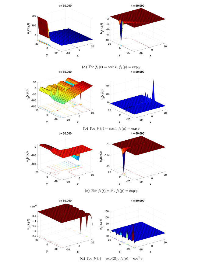
Fig. 2. (a) Single soliton, (b) Elastic multisolitons, (c) Single soliton, and (d) Multisolitons profile of the solutions represented as u2 and h2. |
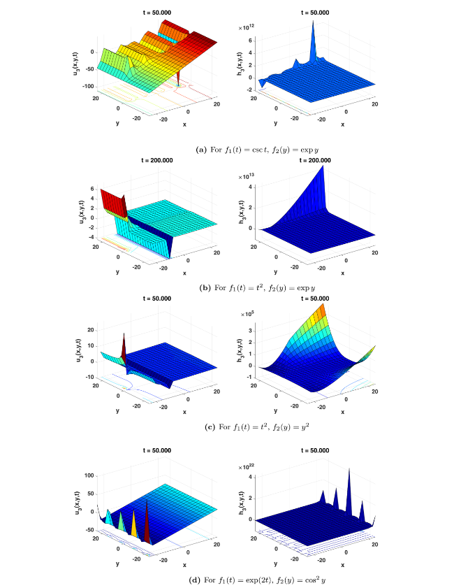
Fig. 3. (a) Flipping and oscillating profile, (b) Kink and single elastic soliton, (c) Single soliton and parabolic, and (d) Multisolitons profile of the expressions expressed by u3 and h3. |

Fig. 4. (a) Asymptotic nature, (b) Flipping and oscillating multisolitons profile, (c) Flapping the flat surface, and (d) h4 creates double sinks. |
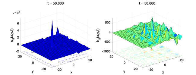
Fig. 5. Multisolitons profiles of u5 and h5 and taking f1(t)=t2 and f2(y)=cos2y. |
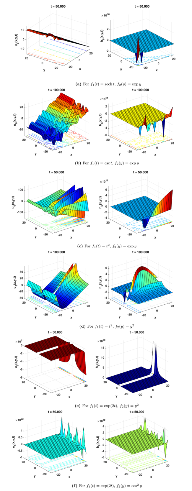
Fig. 6. (a) Doubly solitons, (b) Oscillating multisolitons, (c) Elastics multisolitons, (d) Parabolic nature, (e) Doubly solitons with a bore, and (f) Multisolitons for u6 and h6. |

Fig. 7. (a) Singular kink waves, (b) Multisolitons, (c) Multisolitons, (d) Doubly soliton with a bore for u7 and h7. |
Figure 1: For simulation of the profile, the arbitrary constants are taken as A1=0.60, A2=0.25 with appropriate choices of functions f1(t) while keeping f2(y)=exp y. In sub-figure (a); for f1(t)=sech t, u1 begins with amplitude 0 while variation h1 in surface water of shallow wave shows single soliton. After t≥2.5 interaction of both components is always a single soliton. The behavior profile remains stable. In sub-figure (b), f1(t)=csc t is taken, then u1 and h1 show elastic multisolitons with variation in time. In the sub-figure (c), f1(t)=t2 is chosen, single soliton profile can be observed.
Figure 2: For animation of the surface plots, arbitrary constant C1=0.72 is chosen. Combinations of different choices of f1(t) and f2(y) are chosen for expressions u2, h2. For such choices four profiles are plotted which are given as follows:
In sub-figure (a), for f1(t)=sech t, f2(y)=exp y, flat surface of u2 oscillates initially. After, t≥2.5 single soliton behavior can be obtained.
In sub-figure (b), for f1(t)=csc t, f2(y)=exp y, due to the presence of f1(t)=csc t nature of wave is governed by nature of f1(t). It concludes that the f1(t) plays its crucial role to decide the nature of wave. Flipping as well as oscillation of flat surface of u2 comprising multisolitons can be observed in animations as t increases.
In sub-figure (c), for f1(t)=t2, f2(y)=exp y profile reflects single soliton behavior while in (d), for f1(t)=exp (2t), f2(y)=cos2 y, multisolitons are there.
Figure 3: For simulation of the profile in sub-figure (a), f1(t)=csc t, f2(y)=exp y, and constants are taken as C2=0.42 and C3=0.91 with suitable choice of f1(t) and f2(y). Nature of profile given in Fig. 2(b) is similar to 3(a). In sub-figures (b), for f1(t)=t2, f2(y)=exp y, kink and single elastic soliton can be seen, in (c), for f1(t)=t2, f2(y)=y2, single soliton and parabolic nature appear, and in (d) multisolitons profile of the expressions expressed by u3 and h3 with choices of f1(t)=exp (2t), f2(y)=cos2y, can be observed.
Figure 4: The authors have taken k1=0.27 and C8=0.54 for simulation. In sub-figure (a), for f1(t)=sech t, f2(y)=exp y, the x-component u4 of shallow wave shows asymptotic nature while h4 creates a bore at (x=25,y=−25). In sub-figure (b), for the choice of f1(t)=csct, f2(y)=exp y, u4 flips and oscillate creating doubly solitons while surface animation of h4 reflects multisolitons profile of with respect to variation in time. In sub-figure (c), for f1(t)=t2, ${{f}_{2}}\left( y \right)=\exp y$, h4 creates a sink at (−22.31,−25). In (d), for f1(t)=exp(2t), f2(y)=y2, u4 is stationary with respect to time while h4 steepening of water wave creates a bore as shown here. It means large amplitude instability of waves can be seen in the profile.
Figure 6: Profiles of this figure are presented by Eqs. (38) and (39). The animation frames are traced for u6 and h6. Profiles reflect doubly solitons (in sub figure (a) with f1(t)=secht, f2(y)=exp y), oscillating multisolitons (in sub figure (b) with f1(t)=csc t, f2(y)=exp y), elastic multisolitons (in sub figure (c) with f1(t)=t2, f2(y)=exp y), parabolic (in sub figure (d) with f1(t)=t2, f2(y)=y2), doubly-soliton with a bore (in sub figure (e) with f1(t)=exp(2t), f2(y)=y2) and multisolitons (in sub figure (f) with f1(t)=exp(2t), f2(y)=cos2y), nature for u6 and h6. Adequate choices of constants are a=0.95 and C10=0.34.
Figure 7: Surface plots depicted here are represented mathematically in Eqs. (45) and (46). For simulation, the authors took C12=0.01, C13=0.04, and C14=0.16 in MATLAB code by capturing dominated behavior of animation. Profiles are explored in sub-figures (a)-(d). In sub-figure (a), f1(t)=secht, f2(y)=exp y is taken in u7, it shows singular kink waves and h7 creates a large amplitude instability at (−25,−25), while in (b), for f1(t)=csc t, f2(y)=exp y, multisoliton profile can be appeared. In sub-figure (c) for f1(t)=exp(2t), f2(y)=cos2y, multisolitons i.e. many valued profiles can be seen. In (d), authors have taken f1(t)=exp(2t), f2(y)=y2, profiles are doubly solitons with a bore is observed. Solitons are waves that have only one crest. Self-focusing, an inherently nonlinear process, cancels out a waves natural tendency to spread as it propagates, resulting in them.
5. Conclusions
In summary, two more general solutions and five different solutions from existing literature are obtained successfully by using the STM via Lie group theory. Solutions are obtained for the (2+1)-DLWEs, which propagate in an infinitely long channel with constant depth and can be observed in an open sea or in wide channels. The invariance property of the STM via one-parameter Lie group theory is utilized, and it reduces one fewer number of independent variables from a system of DLWEs at each level. The repeated use of the STM transformed the system of DLWEs into a new system of ODEs. Under adequate restrictions, this system of ODEs is solved. Furthermore, during the similarity reductions, the intermediate integrations are restricted like ${{f}_{3}}\left( t \right)=\frac{{{a}_{0}}}{2}f_{1}^{\prime }\left( t \right)$ only, but no restriction is imposed on f1(t) and f2(y), whereas Sharma et al. [37] restricted f1(t) as f1(t)=t2 and f2(y)=1 and Kumar et al. [36] have taken particular choice of f2(y)=1 and f2(y)=d to generate optimal classes of subalgebra for the system (1). All the analytical solutions are extended with numerical simulations to plot their animations with respect to the variation in space and time. As a result, dynamical behavior of the solutions exhibits elastic multisolitons, single soliton, doubly solitons, stationary, kink and parabolic nature (in Fig. 1, Fig. 2, Fig. 3, Fig. 4, Fig. 5, Fig. 6, Fig. 7). Results are significant since some of the results derived in the previous findings [36], [37] are deduced in the comparison section. Other results in all the existing literature are different from those in this work. This research can help to solve such NEEs occurring in ocean sciences and water waves theory.
Availability of data and materials
Data sharing does not apply to this article.
Funding
Not applicable.
Disclosure statement
We wish to assure that this publication is free of any known conflicts of interest.
Declaration of Competing Interest
Authors declare that they have no conflicts of interest for the manuscript “On similarity solutions to (2+1)-dispersive long-wave equations”
