
1. Introduction
Nonlinear sciences have evolved into an important frontier subject in contemporary scientific research by merging mathematical and physical sciences [1], [2], [3], [4], [5], [6], [7], [8], [9], [10], [11], [12], [13], [14], [15], [16], [17], [18], [19]. Many researchers have developed a strong desire to work on exact solutions to nonlinear evolution equations in recent decades [20], [21], [22], [23], [24], [25], [26], [27], [28], [29], [30], [31], [32], [33], [34], [35], and it is worthwhile to seek for obtaining analytical solutions to these equations because of their importance in many scientific and engineering applications. a number of conventional methods have been proposed, including Kudryashov method [36], inverse scattering transform method [37], Bäcklund transformation method, the truncated Painlevé expansion [38], GERF method [39], [40], Lie classical method [41], [42], [43], [44], [45], [46], [47], [48], Darboux transformation method [49], Hirota bilinear method [50], [51], [52], [53], and many others to find the analytical solutions of these NLEES.
The (3+1)-dimensional B-KP equation has been established as one of the most important non-linear evolution equations, as
${{u}_{xxxy}}+\alpha {{\left( {{u}_{x}}{{u}_{y}} \right)}_{x}}+{{\left( {{u}_{x}}+{{u}_{y}}+{{u}_{z}} \right)}_{t}}-\left( {{u}_{xx}}+{{u}_{zz}} \right)=0,$
which depict the evolution of quasi-one dimensional shallow water waves with insignificant effects of surface tension and viscosity. This equation has a wide range of applications in nonlinear sciences, including ferromagnetics, surface and internal oceanic waves, Bose-Einstein condensation, plasma physics, nonlinear optics, and string theory, to mention a few. Because of the relevance of the weakly coupled B-Type KP equation, several researchers have used a variety of techniques to solve it. In Ref. [54], Huang et al. find the soliton solutions for the governing equation by applying bilinear Bäcklund transformations. Wazwaz [55] determined soliton solutions of the given equation by employing the simplified Hereman-Nuseir form. A generalized form of the (3+1)-dimensional B-KP equation was presented by Kaur and Wazwaz in [56] and explored bright-dark lump wave solutions. In [57], lump, breather, and solitary wave solutions have been found for the new reduced form of the generalized B-KP equation. A more generalized version of this equation was also handled by Kumar et al. [58] and found group-invariant solutions using Lie symmetry analysis. In [59], Xiong et al. used ZN-KP hierarchy method and acquire a new weakly coupled (3+1)-dimensional B-KP equations
$\begin{matrix} {} & {{u}_{xxxy}}+\alpha {{\left( {{u}_{x}}{{u}_{y}} \right)}_{x}}+{{\left( {{u}_{x}}+{{u}_{y}}+{{u}_{z}} \right)}_{t}}-\left( {{u}_{xx}}+{{u}_{zz}} \right)=0, \\ {} & {{v}_{xxxy}}+\alpha {{\left( {{v}_{x}}{{u}_{y}} \right)}_{x}}+\alpha {{\left( {{u}_{x}}{{v}_{y}} \right)}_{x}}+{{\left( {{v}_{x}}+{{v}_{y}}+{{v}_{z}} \right)}_{t}}-\left( {{v}_{xx}}+{{v}_{zz}} \right)=0. \\\end{matrix}$
where u and v are the unknown functions. The challenge of investigating invariant solutions for the weakly coupled (2+1)-dimensional B-KP Eq. (2) obtained by substituting z=x into the equation is presented here. This research is intended to seek the group-invariant solutions of a given weakly coupled B-KP equations [59]
$\begin{matrix} {} & {{u}_{xxxy}}+\alpha {{u}_{xx}}{{u}_{y}}+\alpha {{u}_{x}}{{u}_{yx}}+2{{u}_{xt}}+{{u}_{yt}}=0, \\ {} & {{v}_{xxxy}}+\alpha {{v}_{xx}}{{u}_{y}}+\alpha {{v}_{x}}{{u}_{yx}}+\alpha {{u}_{xx}}{{v}_{y}}+\alpha {{u}_{x}}{{v}_{yx}}+2{{v}_{xt}}+{{v}_{yt}}=0. \\\end{matrix}$
Recently, Lumps, soliton solutions, and rational analytical solutions of the considered weakly coupled B-KP equation were explored by Xiong et al. [59]. In this work, we seek to establish an optimal system of Lie subalgebras of weakly coupled B-KP Eq. (3), which will effectively assist to classify the group-invariant solutions, based on the work of the aforementioned authors. After that, each constituent of the optimal system is provided a reduced equation. Using the Lie classical technique, we will be able to determine a variety of new analytical solutions to the governing system, as well as distinct dynamical wave forms of achieved solutions. Our best knowledge shows that the solutions presented in this article have never been published previously. One of the most efficient ways of studying the analytical solutions of nonlinear PDEs emerging in a wide range of disciplines is the theory of Lie groups. Over the previous few decades, Several textbooks and research papers [60], [61], [62], [63] have studied the detailed summary and application of Lie symmetry analysis.
The following is a description of the remaining paper: In Section 2, some basic terminology of Lie symmetry is employed to derive the commutator table, infinitesimal generators, and invariance criterion. By taking advantage of the obtained symmetries, the invariant groups of Eq. (3) are presented. Section 3 shows the derivation of an optimal system of symmetry subalgebras to the weakly coupled B-KP Eq. (3). The Lie symmetry technique is applied to the symmetry reductions of the Eq. (3) and to obtain the invariant solutions in Section 4. Section 5 discusses some of the analysis of graphic results and their dynamical behaviors. Finally, the conclusion and future scope of this research work are given.
2. Symmetry analysis for coupled equation
The construction of invariant solutions is the main purpose of Lie symmetries in nonlinear differential equations. This reduces the number of independent variables in a system of non-linear PDEs that already exists. As a consequence, the streamlined system with fewer variables is simple to solve. These findings are crucial for defining dynamical properties and describing the wave structures of particular singularities. The weakly coupled BKP system is more complex to solve precisely because of its highly nonlinear behavior. Here we employ the Lie classical method to determine the infinitesimal generators, commutation relation, and optimal classification in order to find the symmetry reductions of Eq. (3). To achieve this goal, assume that Eq. (3) remains invariant with the one-parameter transformations,
$\begin{matrix} x_{a}^{*} & ={{x}_{a}}+\epsilon {{\xi }_{a}}\left( {{x}_{a}},{{u}_{b}} \right)+O\left( {{\epsilon }^{2}} \right), \\ u_{b}^{*} & ={{u}_{b}}+\epsilon {{\eta }_{b}}\left( {{x}_{a}},{{u}_{b}} \right)+O\left( {{\epsilon }^{2}} \right). \\\end{matrix}$
Here ξ1, ξ2, ξ3, η1 and η2 are infinitesimals generators with a small parameter ϵ<<1 which conserve the invariance of system. The infinitesimal point symmetries of Eq. (3) consists of a set of vector fields given by
$V=\underset{a=1}{\overset{3}{\mathop \sum }}\,{{\xi }_{a}}\frac{\partial }{\partial {{x}_{a}}}+\underset{b=1}{\overset{2}{\mathop \sum }}\,{{\eta }_{b}}\frac{\partial }{\partial {{u}_{b}}},$
where ξ1, ξ2, ξ3 depends on x, y, t and η1 and η2 depends on x, y, t, u, v. For the infinitesimal generators defined above, the invariance criterion is given as
$\left.\operatorname{Pr}^{(4)} \mathrm{V}(\triangle)\right|_{\triangle=0}=0 $
Here Pr(4)V is forth order prolongations defined as
$\begin{aligned} \operatorname{Pr}^{(4)} \mathrm{V}\left(\triangle_{1}\right)= & \mathrm{V}+\eta_{1}^{x} \frac{\partial}{\partial u_{x}}+\eta_{1}^{y} \frac{\partial}{\partial u_{y}}+\eta_{1}^{t} \frac{\partial}{\partial u_{t}} \\ & +2 \eta_{1}^{x t} \frac{\partial}{\partial u_{x t}}+\eta_{1}^{y t} \frac{\partial}{\partial u_{y t}}+\alpha u_{y} \eta_{1}^{x x} \frac{\partial}{\partial u_{x x}} \\ & +\alpha u_{x x} \eta_{1}^{y} \frac{\partial}{\partial u_{y}}+\alpha u_{x} \eta_{1}^{y x} \frac{\partial}{\partial u_{y x}} \\ & +\alpha u_{y x} \eta_{1}^{x} \frac{\partial}{\partial u_{x}}+\eta_{1}^{x x x y} \frac{\partial}{\partial u_{x x x y}} \ldots \\ \operatorname{Pr}^{(4)} \mathrm{V}\left(\triangle_{2}\right)= & \mathrm{V}+\eta_{1}^{x} \frac{\partial}{\partial u_{x}}+\eta_{1}^{y} \frac{\partial}{\partial u_{y}}+\eta_{2}^{x} \frac{\partial}{\partial u_{x}}+\eta_{2}^{y} \frac{\partial}{\partial u_{y}} \\ & +\eta_{2}^{t} \frac{\partial}{\partial u_{t}}+2 \eta_{2}^{x t} \frac{\partial}{\partial v_{x t}}+\eta_{2}^{y t} \frac{\partial}{\partial v_{y t}}+\alpha u_{y} \eta_{2}^{x x} \frac{\partial}{\partial v_{x x}} \\ & +\alpha v_{x x} \eta_{1}^{y} \frac{\partial}{\partial u_{y}}+\alpha v_{x} \eta_{1}^{y x} \frac{\partial}{\partial u_{y x}}+\alpha u_{y x} \eta_{2}^{x} \frac{\partial}{\partial v_{x}} \\ & +\alpha u_{x x} \eta_{2}^{y} \frac{\partial}{\partial v_{y}}+\alpha v_{y} \eta_{1}^{x x} \frac{\partial}{\partial u_{x x}}+\alpha u_{x} \eta_{2}^{y x} \frac{\partial}{\partial v_{y x}} \\ & +\alpha v_{y x} \eta_{1}^{x} \frac{\partial}{\partial u_{x}}+\eta_{2}^{x x x y} \frac{\partial}{\partial v_{x x x y}} \ldots \end{aligned}$
Applying the forth prolongation transformation to Eq. (3), we obtain invariant equations as follows
$\begin{matrix} {} & \eta _{1}^{xxxy}+\alpha \eta _{1}^{xx}{{u}_{y}}+\alpha {{u}_{xx}}\eta _{1}^{y}+\alpha \eta _{1}^{x}{{u}_{yx}}+\alpha {{u}_{x}}\eta _{1}^{yx}+2\eta _{1}^{xt}+\eta _{1}^{yt}=0, \\ {} & \eta _{2}^{xxxy}+\alpha \eta _{2}^{xx}{{u}_{y}}+\alpha {{v}_{xx}}\eta _{1}^{y}+\alpha \eta _{2}^{x}{{u}_{yx}}+\alpha {{v}_{x}}\eta _{1}^{yx}+\alpha {{u}_{xx}}\eta _{2}^{y}+\alpha \eta _{1}^{xx}{{v}_{y}}+\alpha {{v}_{yx}}\eta _{1}^{x} \\ {} & +\alpha \eta _{1}^{x}{{v}_{yx}}+2\eta _{2}^{xt}+\eta _{2}^{yt}=0. \\\end{matrix}$
Next, with the help of invariant condition, we acquire the following overdetermined equations about ξ1, ξ2, ξ3, η1, η2
$\begin{array}{l} \left(\xi_{1}\right)_{u}=0,\left(\xi_{1}\right)_{v}=0,\left(\xi_{1}\right)_{x}=\frac{1}{3}\left(\xi_{3}\right)_{t},\left(\xi_{1}\right)_{t, t}=0,\left(\xi_{1}\right)_{y}=0 \\ \left(\xi_{2}\right)_{t}=0,\left(\xi_{2}\right)_{v}=0,\left(\xi_{2}\right)_{x}=0,\left(\xi_{2}\right)_{y}=\frac{1}{3}\left(\xi_{3}\right)_{t},\left(\xi_{2}\right)_{u}=0 \\ \left(\xi_{3}\right)_{u}=0,\left(\xi_{3}\right)_{v}=0,\left(\xi_{3}\right)_{x}=0,\left(\xi_{3}\right)_{y}=0,\left(\xi_{3}\right)_{t, t}=0 \\ \left(\eta_{1}\right)_{u}=-\frac{1}{3}\left(\xi_{3}\right)_{t},\left(\eta_{1}\right)_{v}=0,\left(\eta_{1}\right)_{x}=\frac{\left(\xi_{1}\right)_{t}}{\alpha},\left(\eta_{1}\right)_{y}=\frac{2\left(\xi_{1}\right)_{t}}{\alpha} \\ \left(\eta_{2}\right)_{x}=0,\left(\eta_{2}\right)_{u}=0,\left(\eta_{2}\right)_{t v}=0,\left(\eta_{2}\right)_{v v}=0,\left(\eta_{2}\right)_{y}=0 \end{array}$
Therefore, the Lie symmetry group of weakly coupled B-KP Eq. (3) results in the following generators with functional coefficients as
$\begin{array}{ll} \xi_{1}=\frac{c_{1} x}{3}+c_{4} t+c_{5}, \quad \xi_{2}=\frac{c_{1} y}{3}+c_{3}, & \xi_{3}=c_{1} t+c_{2} \\ \eta_{1}=\frac{c_{4} x}{\alpha}-\frac{c_{1} u}{3}+\frac{2 c_{4} y}{\alpha}+f_{2}(t), & \eta_{2}=c_{6} v+f_{1}(t) \end{array}$
where f1(t) and f2(t) are arbitrary smooth functions. The Lie algebra are determined by these eight vectors
$V={{V}_{1}}+{{V}_{2}}+{{V}_{3}}+{{V}_{4}}+{{V}_{5}}+{{V}_{6}}+{{V}_{7}}\left( {{f}_{1}}\left( t \right) \right)+{{V}_{8}}\left( {{f}_{2}}\left( t \right) \right),$
Where
$\begin{aligned} \mathrm{V}_{1} & =\frac{x}{3} \frac{\partial}{\partial x}+\frac{y}{3} \frac{\partial}{\partial y}+t \frac{\partial}{\partial t}-\frac{u}{3} \frac{\partial}{\partial u}, \quad \mathrm{~V}_{2}=\frac{\partial}{\partial t}, \quad \mathrm{~V}_{3}=\frac{\partial}{\partial y} \\ \mathrm{~V}_{4} & =t \frac{\partial}{\partial x}+\frac{x}{\alpha} \frac{\partial}{\partial u}+\frac{2 y}{\alpha} \frac{\partial}{\partial u} \\ \mathrm{~V}_{5} & =\frac{\partial}{\partial x} \quad \mathrm{~V}_{6}=v \frac{\partial}{\partial v} \quad \mathrm{~V}_{7}\left(f_{1}(t)\right)=f_{1}(t) \frac{\partial}{\partial v} \\ \mathrm{~V}_{8}\left(f_{2}(t)\right) & =f_{2}(t) \frac{\partial}{\partial u} \end{aligned}$
Following these infinitesimal generators, we obtain eight Lie groups of point transformation recognized by Eq. (3)
$\begin{aligned} \mathscr{G}_{1}:(x, y, t, u, v) & \rightarrow\left(x e^{\epsilon}, y e^{\epsilon}, t e^{3 \epsilon}, u e^{-\epsilon}, v\right) \\ \mathscr{G}_{2}:(x, y, t, u, v) & \rightarrow(x, y, t+\epsilon, u, v) \\ \mathscr{G}_{3}:(x, y, t, u, v) & \rightarrow(x, y+\epsilon, t, u, v) \\ \mathscr{G}_{4}:(x, y, t, u, v) & \rightarrow\left(x+t \epsilon, y, t, u+\frac{(x+2 y) \epsilon}{\alpha}, v\right) \\ \mathscr{G}_{5}:(x, y, t, u, v) & \rightarrow(x+\epsilon, y, t, u, v) \\ \mathscr{G}_{6}:(x, y, t, u, v) & \rightarrow\left(x, y, t, u, v e^{\epsilon}\right) \\ \mathscr{G}_{7}:(x, y, t, u, v) & \rightarrow\left(x, y, t, u, v+\epsilon f_{1}(t)\right) \\ \mathscr{G}_{8}:(x, y, t, u, v) & \rightarrow\left(x, y, t, u+\epsilon f_{2}(t), v\right) \end{aligned}$
where ${{\mathcal{G}}_{2}}$ is known as time translation, ${{\mathcal{G}}_{3}}$, ${{\mathcal{G}}_{5}}$ is named as space translation, and ϵ is the group parameter. Based on the above transformations, different solutions ui, vi of Eq. (3) can be find as
$\begin{array}{ll} \mathfrak{u}_{1}=e^{\epsilon} g_{1}\left(x e^{-\epsilon}, y e^{-\epsilon}, t e^{-3 \epsilon}\right), & \mathrm{v}_{1}=g_{2}\left(x e^{-\epsilon}, y e^{-\epsilon}, t e^{-3 \epsilon}\right). \\ \mathfrak{u}_{2}=g_{1}(x, y, t-\epsilon), & \mathrm{v}_{2}=g_{2}(x, y, t-\epsilon) \\ \mathfrak{u}_{3}=g_{1}(x, y-\epsilon, t), & \mathrm{v}_{3}=g_{2}(x, y-\epsilon, t). \\ \mathfrak{u}_{4}=-\frac{(x+2 y) \epsilon}{\alpha}+g_{1}(x-t \epsilon, y, t), & \mathrm{v}_{4}=g_{2}(x-t \epsilon, y, t). \\ \mathfrak{u}_{5}=g_{1}(x-\epsilon, y, t), & \mathrm{v}_{5}=g_{2}(x-\epsilon, y, t). \\ \mathfrak{u}_{6}=g_{1}(x, y, t), & \mathrm{v}_{6}=e^{-\epsilon} g_{2}(x, y, t). \\ \mathfrak{u}_{7}=g_{1}(x, y, t), & \mathrm{v}_{7}=-\epsilon f_{1}(t)+g_{2}(x, y, t). \\ \mathfrak{u}_{8}=-\epsilon f_{2}(t)+g_{1}(x, y, t), & \mathrm{v}_{8}=g_{2}(x, y, t). \end{array}$
One can construct numerous solutions of Eq. (3) by selecting different values of arbitrary constants.
3. Optimal system
This section discuss the construction of the 1-D optimal system of subalgebra admitted by Eq. (3) to drive more invariant solutions. To construct it, we simplify the expression of Lie algebra. For this, adjoint transformation is constructed by the relation
$\begin{matrix} Ad\left( exp\left( \epsilon {{V}_{0}} \right) \right){{W}_{0}} & = & \underset{n=0}{\overset{\infty }{\mathop \sum }}\,\frac{{{\epsilon }^{n}}}{n!}{{\left( ad{{V}_{0}} \right)}^{n}}\left( {{W}_{0}} \right)={{W}_{0}}-\epsilon \left[ {{V}_{0}},{{W}_{0}} \right] \\ {} & {} & +\frac{{{\epsilon }^{2}}}{2}\left[ {{V}_{0}},\left[ {{V}_{0}},{{W}_{0}} \right] \right]-\ldots \\ \end{matrix}$
$\begin{aligned} A_{1} & =\operatorname{Ad}\left(e^{\epsilon_{1} \mathrm{v}_{1}}\right)=\left(\begin{array}{cccccccc} 1 & 0 & 0 & 0 & 0 & 0 & 0 & 0 \\ 0 & e^{\epsilon_{1}} & 0 & 0 & 0 & 0 & 0 & 0 \\ 0 & 0 & e^{\frac{\epsilon_{1}}{3}} & 0 & 0 & 0 & 0 & 0 \\ 0 & 0 & 0 & e^{-\frac{2 \epsilon_{1}}{3}} & 0 & 0 & 0 & 0 \\ 0 & 0 & 0 & 0 & e^{\frac{\epsilon_{1}}{3}} & 0 & 0 & 0 \\ 0 & 0 & 0 & 0 & 0 & 1 & 0 & 0 \\ 0 & 0 & 0 & 0 & 0 & 0 & e^{-\epsilon_{1}} & 0 \\ 0 & 0 & 0 & 0 & 0 & 0 & 0 & e^{-\epsilon_{1}} \end{array}\right) \end{aligned}$
$A_{2}=A d\left(e^{\epsilon_{2} V_{2}}\right)=\left(\begin{array}{cccccccc} 1 & -\epsilon_{2} & 0 & 0 & 0 & 0 & 0 & 0 \\ 0 & 1 & 0 & 0 & 0 & 0 & 0 & 0 \\ 0 & 0 & 1 & 0 & 0 & 0 & 0 & 0 \\ 0 & 0 & 0 & 1 & -\epsilon_{2} & 0 & 0 & 0 \\ 0 & 0 & 0 & 0 & 1 & 0 & 0 & 0 \\ 0 & 0 & 0 & 0 & 0 & 1 & 0 & 0 \\ 0 & 0 & 0 & 0 & 0 & 0 & e^{-\epsilon_{2}} & 0 \\ 0 & 0 & 0 & 0 & 0 & 0 & 0 & e^{-\epsilon_{2}} \end{array}\right) $
$A_{3}=A d\left(e^{\epsilon_{3} v_{3}}\right)=\left(\begin{array}{cccccccc} 1 & 0 & -\frac{\epsilon_{3}}{3} & 0 & 0 & 0 & 0 & 0 \\ 0 & 1 & 0 & 0 & 0 & 0 & 0 & 0 \\ 0 & 0 & 1 & 0 & 0 & 0 & 0 & 0 \\ 0 & 0 & 0 & 1 & 0 & 0 & 0 & -\frac{2 \epsilon_{3}}{\alpha} \\ 0 & 0 & 0 & 0 & 1 & 0 & 0 & 0 \\ 0 & 0 & 0 & 0 & 0 & 1 & 0 & 0 \\ 0 & 0 & 0 & 0 & 0 & 0 & 1 & 0 \\ 0 & 0 & 0 & 0 & 0 & 0 & 0 & 1 \end{array}\right), $
$A_{4}=\operatorname{Ad}\left(e^{\epsilon_{4} \mathrm{~V}_{4}}\right)=\left(\begin{array}{cccccccc} 1 & 0 & 0 & \frac{2 \epsilon_{4}}{3} & 0 & 0 & 0 & 0 \\ 0 & 1 & 0 & 0 & \epsilon_{4} & 0 & 0 & 0 \\ 0 & 0 & 1 & 0 & 0 & 0 & 0 & \frac{2 \epsilon_{4}}{\alpha} \\ 0 & 0 & 0 & 1 & 0 & 0 & 0 & 0 \\ 0 & 0 & 0 & 0 & 1 & 0 & 0 & \frac{\epsilon_{4}}{\alpha} \\ 0 & 0 & 0 & 0 & 0 & 1 & 0 & 0 \\ 0 & 0 & 0 & 0 & 0 & 0 & 1 & 0 \\ 0 & 0 & 0 & 0 & 0 & 0 & 0 & 1 \end{array}\right), $
$A_{5}=\operatorname{Ad}\left(e^{\epsilon_{5} \mathrm{~V}_{5}}\right)=\left(\begin{array}{cccccccc} 1 & 0 & 0 & 0 & -\frac{\epsilon_{5}}{3} & 0 & 0 & 0 \\ 0 & 1 & 0 & 0 & 0 & 0 & 0 & 0 \\ 0 & 0 & 1 & 0 & 0 & 0 & 0 & 0 \\ 0 & 0 & 0 & 1 & 0 & 0 & 0 & -\frac{\epsilon_{5}}{\alpha} \\ 0 & 0 & 0 & 0 & 1 & 0 & 0 & 0 \\ 0 & 0 & 0 & 0 & 0 & 1 & 0 & 0 \\ 0 & 0 & 0 & 0 & 0 & 0 & 1 & 0 \\ 0 & 0 & 0 & 0 & 0 & 0 & 0 & 1 \end{array}\right), $
$A_{6}=\operatorname{Ad}\left(e^{\epsilon_{6} \mathrm{v}_{6}}\right)=\left(\begin{array}{llllllll} 1 & 0 & 0 & 0 & 0 & 0 & 0 & 0 \\ 0 & 1 & 0 & 0 & 0 & 0 & 0 & 0 \\ 0 & 0 & 1 & 0 & 0 & 0 & 0 & 0 \\ 0 & 0 & 0 & 1 & 0 & 0 & 0 & 0 \\ 0 & 0 & 0 & 0 & 1 & 0 & 0 & 0 \\ 0 & 0 & 0 & 0 & 0 & 1 & 0 & 0 \\ 0 & 0 & 0 & 0 & 0 & 0 & e^{\epsilon_{6}} & 0 \\ 0 & 0 & 0 & 0 & 0 & 0 & 0 & 1 \end{array}\right), $
$A_{7}=\operatorname{Ad}\left(e^{\epsilon_{7} \mathbb{V}_{7}}\right)=\left(\begin{array}{cccccccc} 1 & 0 & 0 & 0 & 0 & 0 & \epsilon_{7} & 0 \\ 0 & 1 & 0 & 0 & 0 & 0 & \epsilon_{7} & 0 \\ 0 & 0 & 1 & 0 & 0 & 0 & 0 & 0 \\ 0 & 0 & 0 & 1 & 0 & 0 & 0 & 0 \\ 0 & 0 & 0 & 0 & 1 & 0 & 0 & 0 \\ 0 & 0 & 0 & 0 & 0 & 1 & -\epsilon_{7} & 0 \\ 0 & 0 & 0 & 0 & 0 & 0 & 1 & 0 \\ 0 & 0 & 0 & 0 & 0 & 0 & 0 & 1 \end{array}\right), $
$A_{8}=A d\left(e^{\epsilon_{8} \mathrm{v}_{8}}\right)=\left(\begin{array}{llllllll} 1 & 0 & 0 & 0 & 0 & 0 & 0 & \epsilon_{8} \\ 0 & 1 & 0 & 0 & 0 & 0 & 0 & \epsilon_{8} \\ 0 & 0 & 1 & 0 & 0 & 0 & 0 & 0 \\ 0 & 0 & 0 & 1 & 0 & 0 & 0 & 0 \\ 0 & 0 & 0 & 0 & 1 & 0 & 0 & 0 \\ 0 & 0 & 0 & 0 & 0 & 1 & 0 & 0 \\ 0 & 0 & 0 & 0 & 0 & 0 & 1 & 0 \\ 0 & 0 & 0 & 0 & 0 & 0 & 0 & 1 \end{array}\right). $
Table 1. Commutator table for the weakly coupled B-KP Eq. (3). |
| [Vi,Vj] | V1 | V2 | V3 | V4 | V5 | V6 | V7 | V8 |
|---|---|---|---|---|---|---|---|---|
| V1 | 0 | −V2 | $\frac{-V_{3}}{3}$ | $\frac{2}{3} V_{4}$ | $-\frac{V_{5}}{3}$ | 0 | $\mathrm{v}_{7}\left(t f_{1}^{\prime}\right) $ | $\mathrm{V}_{8}\left(t f_{2}^{\prime}+\frac{f_{2}}{3}\right) $ |
| V2 | V2 | 0 | 0 | V5 | 0 | 0 | $\mathrm{v}_{7}\left(f_{1}^{\prime}\right) $ | $\mathrm{V}_{8}\left(f_{2}^{\prime}\right) $ |
| V3 | $\frac{V_{3}}{3}$ | 0 | 0 | $\frac{2}{\alpha} \mathrm{V}_{8}$ | 0 | 0 | 0 | 0 |
| V4 | $-\frac{2}{3} V_{4}$ | −V5 | $-\frac{2}{\alpha} \mathrm{V}_{8}$ | 0 | $-\frac{1}{\alpha} \mathrm{V}_{8}$ | 0 | 0 | 0 |
| V5 | $\frac{V_{5}}{3}$ | 0 | 0 | $\frac{V_{8}}{\alpha}$ | 0 | 0 | 0 | 0 |
| V6 | 0 | 0 | 0 | 0 | 0 | 0 | −V7 | 0 |
| V7 | $-\mathrm{V}_{7}\left(t f_{1}^{\prime}\right) $ | $-\mathrm{v}_{7}\left(f_{1}^{\prime}\right) $ | $0 | 0 | 0 | V7 | 0 | 0 |
| V8 | $-\mathrm{V}_{8}\left(t f_{2}^{\prime}+\frac{f_{2}}{3}\right) $ | $-\mathrm{v}_{8}\left(f_{2}^{\prime}\right) $ | 0 | 0 | 0 | 0 | 0 | 0 |
Table 2. Adjoint table for the weakly coupled B-KP Eq. (3). |
| [Vi,Vj] | V1 | V2 | V3 | V4 | V5 | V6 | V7 | V8 |
|---|---|---|---|---|---|---|---|---|
| V1 | V1 | $e^{\epsilon} V_{2}$ | $e^{\frac{\epsilon}{3}} V_{3}$ | $e^{\frac{-2 \epsilon}{3}} \mathrm{~V}_{4}$ | $e^{\frac{\epsilon}{3}} \mathrm{~V}_{5}$ | V6 | $e^{-\epsilon} \mathrm{V}_{7}$ | $e^{-\epsilon} \mathrm{V}_{8}$ |
| V2 | V1−ϵV2 | V2 | V3 | V4−ϵV5 | V5 | V6 | $e^{-\epsilon} \mathrm{V}_{7}$ | $e^{-\epsilon} \mathrm{V}_{8}$ |
| V3 | $V_{1}-\frac{\epsilon}{3} V_{3}V3$ | V2 | V3 | $\mathrm{V}_{4}-\frac{2 \epsilon}{\alpha} \mathrm{V}_{8}$ | V5 | V6 | V7 | V8 |
| V4 | $\mathrm{V}_{1}+\frac{2 \epsilon}{3} \mathrm{~V}_{4}$ | V2+ϵV5 | $\mathrm{V}_{3}+\frac{2 \epsilon}{\alpha} \mathrm{V}_{8}$ | V4 | $\mathrm{V}_{5}+\frac{\epsilon}{\alpha} \mathrm{V}_{8}$ | V6 | V7 | V8 |
| V5 | $V_{1}-\frac{\epsilon}{3} V_{5}$ | V2 | V3 | $\mathrm{V}_{4}-\frac{\epsilon}{\alpha} \mathrm{V}_{8}$ | V5 | V6 | V7 | V8 |
| V6 | V1 | V2 | V3 | V4 | V5 | V6 | $e^{\epsilon} \mathrm{V}_{7}$ | V8 |
| V7 | V1+ϵV7 | V2+ϵV7 | V3 | V4 | V5 | $V_{6}-\epsilon V_{7}$ | V7 | V8 |
| V8 | V1+ϵV8 | V2+ϵV8 | V3 | V4 | V5 | V6 | V7 | V8 |
Thus, the general adjoint matrix A is furnished as
$\begin{array}{l} A=\prod_{i=1}^{8} A_{i} \\ =\left(\begin{array}{cccccccc} 1 & -\epsilon_{2} & -\frac{\epsilon_{3}}{3} & \frac{2 \epsilon_{4}}{3} & -\epsilon_{2} \epsilon_{4}-\frac{\epsilon_{5}}{3} & 0 & \epsilon_{7}-\epsilon_{2} \epsilon_{7} & -\frac{2 \epsilon_{3} \epsilon_{4}}{3 \alpha}-\frac{2 \epsilon_{5} \epsilon_{4}}{3 \alpha}-\epsilon_{2} \epsilon_{8}+\epsilon_{8} \\ 0 & e^{\epsilon_{1}} & 0 & 0 & e^{\epsilon_{1}} \epsilon_{4} & 0 & e^{\epsilon_{1}} \epsilon_{7} & e^{\epsilon_{1}} \epsilon_{8} \\ 0 & 0 & e^{\frac{\epsilon_{1}}{3}} & 0 & 0 & 0 & 0 & \frac{2 e^{\frac{\epsilon_{1}}{3}} \epsilon_{4}}{\alpha} \\ 0 & 0 & 0 & e^{-\frac{1}{3}\left(2 \epsilon_{1}\right)} & -e^{-\frac{1}{3}\left(2 \epsilon_{1}\right)} \epsilon_{2} & 0 & 0 & -\frac{2 e^{-\frac{1}{3}\left(2 \epsilon_{1}\right)} \epsilon_{3}}{\alpha}-\frac{e^{-\frac{1}{3}\left(2 \epsilon_{1}\right)} \epsilon_{2} \epsilon_{4}}{\alpha}-\frac{e^{-\frac{1}{3}\left(2 \epsilon_{1}\right)} \epsilon_{5}}{\alpha} \\ 0 & 0 & 0 & 0 & e^{\frac{\epsilon_{1}}{3}} & 0 & 0 & \frac{e^{\frac{\epsilon_{1}}{3}} \epsilon_{4}}{\alpha} \\ 0 & 0 & 0 & 0 & 0 & 1 & -\epsilon_{7} & 0 \\ 0 & 0 & 0 & 0 & 0 & 0 & e^{-\epsilon_{1}-\epsilon_{2}+\epsilon_{6}} & 0 \\ 0 & 0 & 0 & 0 & 0 & 0 & 0 & e^{-\epsilon_{1}-\epsilon_{2}} \end{array}\right) \end{array}$
and the adjoint transformation equation for (3) is determined by
$\begin{array}{l} \left(\begin{array}{llllllll} \alpha_{1} & \alpha_{2} & \alpha_{3} & \alpha_{4} & \alpha_{5} & \alpha_{6} & \alpha_{7} & \alpha_{8} \end{array}\right) \\ \quad=\left(\begin{array}{llllllll} \Gamma_{1} & \Gamma_{2} & \Gamma_{3} & \Gamma_{4} & \Gamma_{5} & \Gamma_{6} & \Gamma_{7} & \Gamma_{8} \end{array}\right). A \end{array} $
where A is a global matrix defined by Eq. (16). Solution of Eq. (17) represent the existence of optimal system element.
Case 1 With ϵ1=0, ϵ2=0, ϵ6=0, Γ1=0, Γ2=1, Γ3=0, Γ4=0, Γ6=0, α1=0, α2=1, α3=0, α4=0, α5=0, α6=0, α7=0, α8=0, we obtain a representative element $\mathfrak{T}$= V2 as follows
$\epsilon_{4}=-\Gamma_{5}, \epsilon_{7}=-\Gamma_{7}, \epsilon_{8}=-\left(\frac{\alpha \Gamma_{8}-\Gamma_{5}^{2}}{\alpha}\right)$
Case 2 With ϵ1=0, ϵ2=0, ϵ6=0, Γ1=1, Γ2=0, Γ6=0, α1=1, α2=0, α3=0, α4=0, α5=0, α6=0, α7=1, α8=1, we obtain a representative element $\mathfrak{T}$= V1+V7+V8 as follows
$\begin{aligned}\epsilon_{3} & =3 \Gamma_{3}, \epsilon_{4}=-\frac{3}{2} \Gamma_{4}, \epsilon_{5}=3 \Gamma_{5}, \epsilon_{7}=1-\Gamma_{7}, \epsilon_{8} \\& =\frac{-2 \alpha \Gamma_{8}+2 \alpha+12 \Gamma_{3} \Gamma_{4}+3 \Gamma_{4} \Gamma_{5}}{2 \alpha}\end{aligned}$
Case 3 With ϵ1=0, ϵ2=0, ϵ6=0, Γ1=0, Γ2=1, Γ3=0, Γ4=0, Γ6=1, Γ7=1, α1=0, α2=1, α3=0, α4=0, α5=0, α6=1, α7=1, α8=1, we obtain a representative element $\mathfrak{T}$=V2+V6+V7+V8 as follows
${{\epsilon }_{4}}=-{{\text{ }\!\!\Gamma\!\!\text{ }}_{5}},{{\epsilon }_{8}}=\frac{-\text{ }\!\!\Gamma\!\!\text{ }_{5}^{2}-\alpha +\alpha {{\text{ }\!\!\Gamma\!\!\text{ }}_{8}}}{\alpha }.$
Case 4 With ϵ1=0, ϵ2=0, ϵ6=0, Γ1=0, Γ2=1, Γ3=1, Γ4=0, Γ6=0, α1=0, α2=1, α3=1, α4=0, α5=1, α6=0, α7=1, α8=1, we obtain a representative element $\mathfrak{T}$=V2+V3+V5+V7+V8 as follows
$\epsilon_{4}=1-\Gamma_{5}, \epsilon_{7}=1-\Gamma_{7}, \epsilon_{7}=1-\Gamma_{7}, \epsilon_{8}=\frac{\Gamma_{5}+\Gamma_{5}^{2}+\alpha-2-\alpha \Gamma_{8}}{\alpha}$
Case 5 With ϵ1=0, ϵ2=0, ϵ6=0, Γ1=1, Γ2=1, Γ6=1, α1=1, α2=1, α3=0, α4=0, α5=1, α6=1, α7=0, α8=0, we obtain the generator $\mathfrak{T}$=V1+V2+V3+V5+V6 as follows
$\begin{array}{l} \begin{aligned} \epsilon_{3} & =3\left(\Gamma_{3}-1\right), \epsilon_{4}=-\frac{\left(3 \Gamma_{4}\right)}{2}, \epsilon_{5}=\frac{-3\left(3 \Gamma_{4}-2 \Gamma_{5}+2\right)}{2}, \epsilon_{7} \\ & =-\Gamma_{7}, \epsilon_{8}=\frac{-2 \alpha \Gamma_{8}+12 \Gamma_{3} \Gamma_{4}+3 \Gamma_{5} \Gamma_{4}-6 \Gamma_{4}}{4 \alpha} \end{aligned} \end{array}$
In the same way, we can obtain the values of ϵi, s for rest of the members of optimal system. Finally, we state that the optimal system of useful symmetry groups to the B-KP system (3) is spanned by
$\begin{matrix} {} & \left( i \right)\;{{V}_{2}},\ \ \left( ii \right)\;{{V}_{4}},\ \ \left( iii \right)\ {{V}_{1}}+{{V}_{6}},\ \ \left( iv \right)\ \ {{V}_{1}}+{{V}_{7}}+{{V}_{8}}, \\ {} & \left( v \right)\ \ {{V}_{2}}+{{V}_{6}}+{{V}_{7}}+{{V}_{8}}, \\ {} & \left( vi \right)\ \ {{V}_{2}}+{{V}_{3}}+{{V}_{5}}+{{V}_{7}}+{{V}_{8}},\ \ \left( vii \right)\;{{V}_{1}}+{{V}_{2}}+{{V}_{3}}+{{V}_{5}}+{{V}_{6}}\ \ \\ {} & \left( viii \right)\;{{V}_{2}}+{{V}_{3}}+{{V}_{5}}+{{V}_{6}}+{{V}_{7}}+{{V}_{8}}. \\ \end{matrix}$
The optimal system of Lie algebras provides a single, dual, triple, quadruple, or combination of some more vectors.
4. Lie symmetry analysis and reduction of B-KP equation
The purpose of this section is to deal with the reductions and find closed-form solutions for the Eq. (3). Solutions are achieved through symmetry reductions that are obtained using new coordinates and taking chains derivatives into consideration. In this connection, the related Lagrange’s equation is
$\frac{dx}{\left( \frac{x}{3}+t+1 \right)}=\frac{dy}{\frac{y}{3}+1}=\frac{dt}{\left( t+1 \right)}=\frac{du}{\frac{x}{\alpha }-\frac{u}{3}+\frac{2y}{\alpha }+{{f}_{2}}\left( t \right)}=\frac{dv}{v+{{f}_{1}}\left( t \right)}.$
Case 1. Reduction with ${{V}_{2}}=\frac{\partial }{\partial t}$
The corresponding invariants of V2 are X=x and Y=y with invariant solution of the form
$u\left( x,y,t \right)=U\left( X,Y \right),\;\;v\left( x,y,t \right)=V\left( X,Y \right),$
Inserting (25) into (3), we get
$\begin{matrix} {} & \alpha {{U}_{X}}{{U}_{XY}}+\alpha {{U}_{Y}}{{U}_{XX}}+{{U}_{XXXY}}=0, \\ {} & \alpha {{V}_{X}}{{U}_{XY}}+\alpha {{U}_{X}}{{V}_{XY}}+\alpha {{V}_{Y}}{{U}_{XX}}+\alpha {{U}_{Y}}{{V}_{XX}}+{{V}_{XXXY}}=0. \\\end{matrix}$
To solve the above system (26), the infinitesimals is found as
$\begin{matrix} {{\xi }_{X}} & ={{b}_{1}}X+{{b}_{2}},\quad \ \ {{\xi }_{Y}}={{h}_{1}}\left( Y \right),\quad \ \ {{\eta }_{U}} \\ {} & =-{{b}_{1}}U+{{b}_{5}},\quad \ {{\eta }_{V}}={{b}_{3}}V+{{b}_{4}}. \\\end{matrix}$
For bi=1, 1≤i≤5, the characteristic equation is
$\frac{dX}{X+1}=\frac{dY}{{{h}_{1}}\left( Y \right)}=\frac{dU}{-U+1}=\frac{dV}{V+1}.$
which acquires
$U\left( X,Y \right)=\frac{X}{{{X}_{0}}}+\frac{{{U}_{1}}\left( {{X}_{1}} \right)}{{{X}_{0}}},\;\;V\left( X,Y \right)=-1+\left( {{X}_{0}} \right){{V}_{1}}\left( {{X}_{1}} \right),$
with ${{X}_{1}}=\left( {{X}_{0}} \right){{e}^{-\int \frac{dY}{{{h}_{1}}\left( Y \right)}}}\text{and}\;{{X}_{0}}=X+1.$ The second reduction of Eq. (3) is
$\begin{array}{l} \begin{array}{l} -2 \alpha U_{1}^{\prime}+2 \alpha U_{1} U_{1}^{\prime}+2 \alpha X_{1}^{2} U_{1}^{\prime} U_{1}^{\prime \prime}-2 X_{1} U_{1}^{\prime 2} \\ \quad+X_{1} U_{1}^{\prime \prime}-X_{1} U_{1} U_{1}^{\prime \prime}+X_{1}^{3} U_{1}^{\prime \prime \prime}=0 \\ 2 \alpha X_{1} U_{1}^{\prime} V_{1}^{\prime}+2 \alpha X_{1}^{2} U_{1}^{\prime \prime} V_{1}^{\prime}+\alpha X_{1} V_{1} U_{1}^{\prime \prime}+(6+\alpha) X_{1} V_{1}^{\prime \prime}-\alpha X_{1} U_{1} V_{1}^{\prime \prime} \\ +2 \alpha X_{1}^{2} U_{1}^{\prime} V_{1}^{\prime \prime}+6 X_{1}^{2} V_{1}^{\prime \prime \prime}+X_{1}^{3} V_{1}^{\prime \prime \prime \prime}=0 \end{array} \end{array}$
Solution of Eq. (30) is obtained as
${{U}_{1}}\left( {{X}_{1}} \right)=\frac{6+\alpha }{\alpha },\quad {{V}_{1}}\left( {{X}_{1}} \right)={{a}_{0}}+{{a}_{1}}{{X}_{1}}+{{a}_{2}}X_{1}^{2}+\frac{{{a}_{3}}}{X_{1}^{3}}.$
Here a0, a1, a2 and a3 are constants. Finally, we get the analytical solution of system (3)
$\begin{aligned} u(x, y, t)= & \frac{x}{x+1}+\frac{\alpha+6}{\alpha(x+1)} \\ v(x, y, t)= & -1+(x+1)\left(a_{0}+a_{1}(x+1) e^{-\int \frac{1}{h_{1}(v)} d y}\right. \\ & \left.+a_{2}(x+1)^{2} e^{-2 \int \frac{1}{n_{1}(v)} d y}+\frac{a_{3} e^{3 \int \frac{1}{h_{1}(x)} d y}}{(x+1)^{3}}\right) \end{aligned}$
Case 2. Reduction with ${{V}_{4}}=t\frac{\partial }{\partial x}+\frac{x}{\alpha }\frac{\partial }{\partial u}+\frac{2y}{\alpha }\frac{\partial }{\partial u}$
For the generator V4, we have Y=y and T=t with similarity functions as
$u\left( x,y,t \right)=\frac{\frac{{{x}^{2}}}{2}+2xy}{\alpha t}+U\left( Y,T \right),\;v\left( x,y,t \right)=V\left( Y,T \right).$
Back substitution of Eq. (33) into Eq. (3) results the following PDE’s
$\begin{matrix} {{U}_{Y}}+T{{U}_{YT}}=0, \\ {{V}_{Y}}+T{{V}_{YT}}=0. \\\end{matrix}$
Solving the above equations for U and V gives
$\begin{matrix} U\left( Y,T \right) & =\int \frac{{{h}_{2}}\left( Y \right)}{T}dY+{{h}_{3}}\left( T \right), \\ V\left( Y,T \right) & =\int \frac{{{h}_{4}}\left( Y \right)}{T}dY+{{h}_{5}}A\left( T \right). \\ \end{matrix}$
Therefore, we attain the solution of (3) as
$\begin{matrix} u\left( x,y,t \right) & =\frac{2\alpha \int {{h}_{2}}\left( y \right)dy+{{x}^{2}}+4xy}{2\alpha t}+{{h}_{3}}\left( t \right), \\ v\left( x,y,t \right) & =\frac{1}{t}\int {{h}_{4}}\left( y \right)dy+{{h}_{5}}\left( t \right). \\\end{matrix}$
Case 3. Reduction with ${{V}_{1}}+{{V}_{6}}=\frac{x}{3}\frac{\partial }{\partial y}+\frac{y}{3}\frac{\partial }{\partial y}+t\frac{\partial }{\partial t}-\frac{u}{3}\frac{\partial }{\partial u}+v\frac{\partial }{\partial v}$
The characteristic equation associated with the admitted operator V1+V6 is
$\frac{dx}{x}=\frac{dy}{y}=\frac{dt}{3t}=\frac{du}{-u}=\frac{dv}{3v}.$
From (37), we get similarity independent variables $X=\frac{x}{\sqrt[3]{t}}$ and $Y=\frac{y}{\sqrt[3]{t}}$ with similarity solution defined as
$\begin{matrix} u\left( x,y,t \right)=\frac{U\left( X,Y \right)}{\sqrt[3]{t}}, \\ \;v\left( x,y,t \right)=tV\left( X,Y \right), \\\end{matrix}$
By using Eq. (38) and (3), we get
$\begin{array}{l} -Y U_{Y Y}-(X+2 Y) U_{X Y}-2 X U_{X X}-4 U_{X}-2 U_{Y}+3 \alpha U_{X} U_{X Y} \\ +3 \alpha U_{Y} U_{X X}+3 U_{X X X Y}=0 \\ 4 V_{X}+3 \alpha V_{X} U_{X Y}+3 \alpha U_{X} V_{X Y}+3 \alpha U_{X} V_{X Y}+3 \alpha U_{Y} V_{X X}+2 V_{Y} \\ +3 V_{X X X Y}-Y V_{Y Y}-(X+2 Y) V_{X Y}-2 X V_{X X}=0 \end{array}$
To solve the system (39), we use the wave transformation ${{X}_{2}}=aX+bY$ with
$U\left( X,Y \right)={{U}_{2}}\left( {{X}_{2}} \right),\;\;V\left( X,Y \right)={{V}_{2}}\left( {{X}_{2}} \right)$
Eq. (40) and (39) gives the following system
$\begin{array}{r} (2 a+b) X_{2} U_{2}^{\prime \prime}+(4 a+2 b) U_{2}^{\prime}-6 \alpha a^{2} b U_{2}^{\prime} U_{2}^{\prime \prime}-3 a^{3} b U_{2}^{\prime \prime \prime}=0 \\ (4 a+2 b) V_{2}^{\prime}+6 \alpha a^{2} b\left(V_{2}^{\prime} U_{2}^{\prime \prime}+U_{2}^{\prime} V_{2}^{\prime \prime}\right)+3 a^{3} b V_{2}^{\prime \prime \prime \prime}-(2 a+b) X_{2} V_{2}^{\prime \prime}=0 \end{array}$
The latter can be simplified to the form
${{U}_{2}}\left( {{X}_{2}} \right)={{a}_{4}}+\frac{6a}{\alpha {{X}_{2}}},\quad {{V}_{2}}\left( {{X}_{2}} \right)={{a}_{5}}+{{a}_{6}}X_{2}^{3}.$
Here a4, a5, a6 are constants. Thus, the invariant solution of system (3) is
$\begin{array}{l} u(x, y, t)=\frac{a_{4}}{\sqrt[3]{t}}+\frac{6 a}{a \alpha x+\alpha b y} \\ v(x, y, t)=t\left(a_{5}+a_{6}\left(\frac{a x}{\sqrt[3]{t}}+\frac{b y}{\sqrt[3]{t}}\right)^{3}\right) \end{array}$
Case 4. Reduction with ${{V}_{1}}+{{V}_{7}}+{{V}_{8}}=\frac{x}{3}\frac{\partial }{\partial y}+\frac{y}{3}\frac{\partial }{\partial y}+t\frac{\partial }{\partial t}-\frac{u}{3}\frac{\partial }{\partial u}+{{f}_{1}}\left( t \right)\frac{\partial }{\partial v}+{{f}_{2}}\left( t \right)\frac{\partial }{\partial u}$
For the generator V1+V7+V8, we can obtain
$\begin{array}{l} u(x, y, t)=\frac{1}{\sqrt[3]{t}}\left(\int \frac{f_{2}(t)}{t^{2 / 3}} d t\right)+\frac{1}{\sqrt[3]{t}} U(X, Y) \\ v(x, y, t)=\int \frac{f_{1}(t)}{t} d t+V(X, Y) \end{array}$
where $X=\frac{x}{\sqrt[3]{t}}$ and $Y=\frac{y}{\sqrt[3]{t}}$. Thus Eq. (3) gets transformed to
$\begin{array}{l} Y U_{Y Y}+(X+2 Y) U_{X Y}+2 X U_{X X}+4 U_{X}+2 U_{Y}-3 \alpha U_{X} U_{X Y} \\ -3 \alpha U_{Y} U_{X X}-3 U_{X X X Y}=0 \\ -2 V_{X}+3 \alpha V_{X} U_{X Y}+3 \alpha U_{X} V_{X Y}+3 \alpha U_{X} V_{X Y}+3 \alpha U_{Y} V_{X X}-V_{Y} \\ +3 V_{X X X Y}-Y V_{Y Y}-(X+2 Y) V_{X Y}-2 X V_{X X}=0 \end{array}$
By using the wave transformation ${{X}_{3}}=aX+bY$ with
$U\left( X,Y \right)={{U}_{3}}\left( {{X}_{3}} \right),\;\;V\left( X,Y \right)={{V}_{3}}\left( {{X}_{3}} \right),$
Eq. (45) converted into the following ODE as
$\begin{array}{l} (2 a+b) X_{3} U_{3}^{\prime \prime}+(4 a+2 b) U_{3}^{\prime}-6 \alpha a^{2} b U_{3}^{\prime} U_{3}^{\prime \prime}-3 a^{3} b U_{3}^{\prime \prime \prime \prime}=0 \\ -(2 a+b) V_{3}^{\prime}+6 \alpha a^{2} b\left(V_{3}^{\prime} U_{3}^{\prime \prime}+U_{3}^{\prime} V_{3}^{\prime \prime}\right)+3 a^{3} b V_{3}^{\prime \prime \prime \prime}-(2 a+b) X_{3} V_{3}^{\prime \prime}=0 \end{array}$
Solving system (47), we can get
${{U}_{3}}\left( {{X}_{3}} \right)={{a}_{7}}+\left( \frac{2a+b}{4{{a}^{2}}b\alpha } \right)X_{3}^{2},\quad {{V}_{3}}\left( {{X}_{3}} \right)={{a}_{8}}.$
Here a7, and a8 are constants. Moving towards the solution of (3)
$\begin{matrix} u\left( x,y,t \right) & =\frac{{{a}_{7}}}{\sqrt[3]{t}}+\frac{\left( 2a+b \right){{\left( ax+by \right)}^{2}}}{4{{a}^{2}}\alpha bt}+\frac{\int \frac{{{f}_{2}}\left( t \right)}{{{t}^{2/3}}}dt}{\sqrt[3]{t}}, \\ v\left( x,y,t \right) & ={{a}_{8}}+\int \frac{{{f}_{1}}\left( t \right)}{t}dt. \\ \end{matrix}$
Case 5. Reduction with ${{V}_{2}}+{{V}_{6}}+{{V}_{7}}+{{V}_{8}}=\frac{\partial }{\partial t}+\left( v+{{f}_{1}}\left( t \right) \right)\frac{\partial }{\partial v}+{{f}_{2}}\left( t \right)\frac{\partial }{\partial u}$
For the generator V2+V6+V7+V8, we get
$\begin{matrix} u\left( x,y,t \right) & =U\left( X,Y \right)+\int {{f}_{2}}\left( t \right)dt,\;v\left( x,y,t \right) \\ {} & ={{e}^{t}}\int {{e}^{-t}}{{f}_{1}}\left( t \right)dt+{{e}^{t}}V\left( X,Y \right), \\ \end{matrix}$
with X=x and Y=y. From Eq. (50) and (3), we accomplish the following pde
$\begin{matrix} {} & \alpha {{U}_{X}}{{U}_{XY}}+\alpha {{U}_{Y}}{{U}_{XX}}+{{U}_{XXXY}}=0, \\ {} & 2{{V}_{X}}+\alpha {{V}_{X}}{{U}_{XY}}+\alpha {{U}_{X}}{{V}_{XY}}+\alpha {{V}_{Y}}{{U}_{XX}}+\alpha {{U}_{Y}}{{V}_{XX}}+{{V}_{Y}}+{{V}_{XXXY}}=0. \\ \end{matrix}$
To reduce system (51), the infinitesimals is found as
${{\xi }_{X}}={{b}_{2}},\quad \ \ {{\xi }_{Y}}={{b}_{1}},\quad \ \ {{\eta }_{U}}={{b}_{5}},\quad \ {{\eta }_{V}}={{b}_{3}}V+{{b}_{4}}.$
For bi=1, 1≤i≤5, thus, we have
$\frac{dX}{1}=\frac{dY}{1}=\frac{dU}{1}=\frac{dV}{V+1}.$
Thus
$U\left( X,Y \right)=Y+{{U}_{4}}\left( {{X}_{4}} \right),\;\;V\left( X,Y \right)=-1+{{e}^{Y}}{{V}_{4}}\left( {{X}_{4}} \right),$
with ${{X}_{4}}=X-Y.$. Inserting (54) into (51), we can get system of ODEs as
$\begin{array}{l} \begin{array}{l} \alpha U_{4}^{\prime \prime}-2 \alpha U_{4}^{\prime} U_{4}^{\prime \prime}-U_{4}^{\prime \prime \prime \prime}=0 \\ V_{4}^{\prime}+\alpha V_{4}^{\prime} U_{4}^{\prime}-2 \alpha V_{4}^{\prime} U_{4}^{\prime \prime}+V_{4}+\alpha V_{4} U_{4}^{\prime \prime}+\alpha V_{4}^{\prime \prime}-2 \alpha U_{4}^{\prime} V_{4}^{\prime \prime}+V_{4}^{\prime \prime \prime}-V_{4}^{\prime \prime \prime \prime}=0 \end{array} \end{array}$
Solution of Eq. (55) leads to
${{U}_{4}}\left( {{X}_{4}} \right)={{a}_{9}}+\frac{6}{\alpha {{X}_{4}}}+\frac{{{X}_{4}}}{2},\quad {{V}_{4}}\left( {{X}_{4}} \right)=0.$
Here a9 is constant. Thus the invariant solution becomes
$\begin{matrix} u\left( x,y,t \right) & ={{a}_{9}}+\frac{6}{\alpha \left( x-y \right)}+\frac{x-y}{2}+y+\int {{f}_{2}}\left( t \right)dt, \\ v\left( x,y,t \right) & =-{{e}^{t}}+{{e}^{t}}\int {{e}^{-t}}{{f}_{1}}\left( t \right)dt. \\ \end{matrix}$
Case 6. Reduction with ${{V}_{2}}+{{V}_{3}}+{{V}_{5}}+{{V}_{7}}+{{V}_{8}}=\frac{\partial }{\partial t}+\frac{\partial }{\partial x}+\frac{\partial }{\partial y}+{{f}_{1}}\left( t \right)\frac{\partial }{\partial v}+{{f}_{2}}\left( t \right)\frac{\partial }{\partial u}$
For the generator V2+V3+V5+V7+V8
$u\left( x,y,t \right)=\int {{f}_{2}}\left( t \right)dt+U\left( X,Y \right),\;v\left( x,y,t \right)=\int {{f}_{1}}\left( t \right)dt+V\left( X,Y \right),$
with X=x−t and Y=y−t. From Eq. (58) and (3), we get
$\begin{matrix} {} & {{U}_{YY}}+3{{U}_{XY}}-\alpha {{U}_{X}}{{U}_{XY}}+2{{U}_{XX}}-\alpha {{U}_{Y}}{{U}_{XX}}-{{U}_{XXXY}}=0, \\ {} & {{V}_{YY}}+3{{V}_{XY}}+2{{V}_{XX}}-\alpha {{V}_{X}}{{U}_{XY}}-\alpha {{U}_{X}}{{V}_{XY}}-\alpha {{V}_{Y}}{{U}_{XX}}-\alpha {{U}_{Y}}{{V}_{XX}}-{{V}_{XXXY}}=0. \\ \end{matrix}$
To span the symmetry group of system (59), the infinitesimals is found as
$\begin{matrix} {{\xi }_{X}} & =\frac{{{b}_{1}}X}{3}+{{b}_{3}},\qquad \qquad \qquad \qquad \quad \;{{\xi }_{Y}}={{b}_{1}}Y+{{b}_{2}}, \\ {{\eta }_{U}} & =-\frac{{{b}_{1}}U}{3}+\frac{2{{b}_{1}}X}{\alpha }+\frac{8{{b}_{1}}Y}{3\alpha }+{{b}_{6}},\quad \ \ \ {{\eta }_{V}}={{b}_{4}}V+{{b}_{5}}, \\ \end{matrix}$
Subcase 6.1 ${{b}_{1}}\ne 0\;\text{and}\ \text{rest}\ \text{all}\;b_{i}^{\prime }s=0$
The associated equation is
$\frac{dX}{\frac{X}{3}}=\frac{dY}{Y}=\frac{dU}{-\frac{U}{3}+\frac{2X}{\alpha }+\frac{8Y}{3\alpha }}=\frac{dV}{0}.$
Solution of Eq. (61) gives
$U\left( X,Y \right)=\frac{3X}{\alpha }+\frac{2Y}{\alpha }+\frac{{{U}_{5}}\left( {{X}_{5}} \right)}{\sqrt[3]{Y}},V\left( X,Y \right)={{V}_{5}}\left( {{X}_{5}} \right),$
with invariant variables ${{X}_{5}}=\frac{X}{{{Y}^{\frac{1}{3}}}}.$ Eq. (62) and (59) provides the following nonlinear ODE as
$\begin{array}{l} 6 \alpha U_{5}^{\prime 2}+X_{5}^{2} U_{5}^{\prime \prime}+4 U_{5}+3 \alpha U_{5} U_{5}^{\prime \prime}+6 X_{5} U_{5}^{\prime} \\ +6 \alpha X_{5} U_{5}^{\prime} U_{5}^{\prime \prime}+12 U_{5}^{\prime \prime \prime}+3 X_{5} U_{5}^{\prime \prime \prime}=0 \\ 4 X_{5} V_{5}^{\prime}+9 \alpha U_{5}^{\prime} V_{5}^{\prime}+6 \alpha X_{5} U_{5}^{\prime \prime} V_{5}^{\prime}+X_{5}^{2} V_{5}^{\prime \prime} \\ +3 \alpha U_{5} V_{5}^{\prime \prime}+6 \alpha X_{5} U_{5}^{\prime} V_{5}^{\prime \prime}+9 V_{5}^{\prime \prime \prime}+3 X_{5} V_{5}^{\prime \prime \prime \prime}=0 \end{array}$
Solution of the above reduced equation is given by
${{U}_{5}}\left( {{X}_{5}} \right)=\frac{12}{\alpha {{X}_{5}}},\quad {{V}_{1}}\left( {{X}_{5}} \right)={{a}_{10}}+\frac{{{a}_{11}}}{X_{5}^{3}}.$
Here a10, a11 are constants. The exact solution constructed for this case is
$\begin{array}{r} u(x, y, t)=\frac{3(x-t)}{\alpha}+\frac{12}{\alpha(x-t)}+\frac{2(y-t)}{\alpha}+\int f_{2}(t) d t \\ v(x, y, t)=a_{10}+\frac{a_{11}(y-t)}{(x-t)^{3}}+\int f_{1}(t) d t \end{array}$
Subcase 6.2 ${{b}_{1}}=0\;\text{and}\ \text{rest}\ \text{all}\;b_{i}^{\prime }s=1$
Solving the equation
$\frac{dX}{1}=\frac{dY}{1}=\frac{dU}{1}=\frac{dV}{V+1}$
leads to the
$U\left( X,Y \right)=Y+{{U}_{6}}\left( {{X}_{6}} \right),V\left( X,Y \right)=-1+{{e}^{Y}}{{V}_{6}}\left( {{X}_{6}} \right),$
with ${{X}_{6}}=\frac{X}{{{Y}^{\frac{1}{3}}}}.$ From Eq. (67) and (59) we obtain
$\begin{array}{l} -\alpha U_{6}^{\prime \prime}+2 \alpha U_{6}^{\prime} U_{6}^{\prime \prime}+U_{6}^{\prime \prime \prime \prime}=0 \\ -V_{6}^{\prime}+\alpha U_{6}^{\prime} V_{6}^{\prime}-2 \alpha U_{6}^{\prime \prime} V_{6}^{\prime}-V_{6}+\alpha V_{6} U_{6}^{\prime \prime}+\alpha V_{6}^{\prime \prime} \\ -2 \alpha U_{6}^{\prime} V_{6}^{\prime \prime}+V_{6}^{\prime \prime \prime}-V_{6}^{\prime \prime \prime \prime}=0 \end{array}$
Eq. (68) is solved as follows
${{U}_{6}}\left( {{X}_{6}} \right)={{a}_{12}}+\frac{{{X}_{6}}}{2}+\frac{6}{\alpha {{X}_{6}}},\quad {{V}_{6}}\left( {{X}_{6}} \right)=0.$
Here a12 is constant. Therefore, one arrives at the solution of (3) as
$\begin{array}{l} u(x, y, t)=a_{12}+\int f_{2}(t) d t-t+\frac{6}{\alpha(x-y)}+\frac{x-y}{2}+y \\ v(x, y, t)=-1+\int f_{1}(t) d t \end{array}$
Case 7. Reduction with ${{V}_{1}}+{{V}_{2}}+{{V}_{3}}+{{V}_{5}}+{{V}_{6}}=\frac{x}{3}\frac{\partial }{\partial y}+\frac{y}{3}\frac{\partial }{\partial y}+t\frac{\partial }{\partial t}-\frac{u}{3}\frac{\partial }{\partial u}+\frac{\partial }{\partial t}+\frac{\partial }{\partial x}+\frac{\partial }{\partial y}+v\frac{\partial }{\partial v}$
The characteristic equation associated with the group generator V1+V2+V3+V5+V6 is
$\frac{dx}{\frac{x}{3}+1}=\frac{dy}{\frac{y}{3}+1}=\frac{dt}{t+1}=\frac{du}{-\frac{u}{3}}=\frac{dv}{v}.$
The similarity form is
$u\left( x,y,t \right)=\frac{U\left( X,Y \right)}{\sqrt[3]{t+1}},\;v\left( x,y,t \right)=\left( t+1 \right)V\left( X,Y \right),$
with $X=\frac{x+3}{\sqrt[3]{3}\sqrt[3]{t+1}}$ and $Y=\frac{y+3}{\sqrt[3]{3}\sqrt[3]{t+1}}$ as invariant variables. From Eq. (72) and (3), we get
$\begin{array}{l} Y U_{Y Y}+X U_{X Y}+2 Y U_{X Y}+2 X U_{X X}+4 U_{X}+2 U_{Y}-3^{\frac{1}{3}} \alpha U_{X} U_{X Y} \\ -3^{\frac{1}{3}} \alpha U_{Y} U_{X X}-U_{X X X Y}=0 \\ 4 V_{X}+3^{\frac{1}{3}} \alpha V_{X} U_{X Y}+3^{\frac{1}{3}} \alpha U_{X} V_{X Y}+3^{\frac{1}{3}} \alpha U_{X} V_{X Y} \\ +3^{\frac{1}{3}} \alpha U_{Y} V_{X X}+2 V_{Y}+V_{X X X Y}-Y V_{Y Y} \\ -X V_{X Y}-2 Y V_{X Y}-2 X V_{X X}=0. \end{array}$
By taking the wave transformation ${{X}_{7}}=aX+bY$
$U\left( X,Y \right)={{U}_{7}}\left( {{X}_{7}} \right),\;\;V\left( X,Y \right)={{V}_{7}}\left( {{X}_{7}} \right),$
we obtain
$\begin{array}{l} \begin{array}{l} (2 a+b) X_{7} U_{7}^{\prime \prime}+(4 a+2 b) U_{7}^{\prime}-2 \times 3^{\frac{1}{3}} a^{2} b \alpha U_{7}^{\prime} U_{7}^{\prime \prime}-a^{3} b U_{7}^{\prime \prime \prime \prime}=0 \\ (4 a+2 b) V_{7}^{\prime}+2 \times 3^{\frac{1}{3}} a^{2} b \alpha\left(V_{7}^{\prime} U_{7}^{\prime \prime}+U_{7}^{\prime} V_{7}^{\prime \prime}\right)+a^{3} b V_{7}^{\prime \prime \prime \prime} \\ -(2 a+b) X_{7} V_{7}^{\prime \prime}=0 \end{array} \end{array}$
Solution for Eq. (75) is given as
${{U}_{7}}\left( {{X}_{7}} \right)={{a}_{13}}+\frac{2\ {{3}^{2/3}}a}{\alpha {{X}_{7}}},\quad {{V}_{7}}\left( {{X}_{7}} \right)={{a}_{14}}+{{a}_{15}}X_{7}^{3}.$
Here a13, a14, a15 are constants. Therefore, we get
$\begin{array}{l} u(x, y, t)=\frac{a_{13}}{\sqrt[3]{t+1}}+\frac{6 a}{\alpha(a(x+3)+b(y+3))} \\ v(x, y, t)=(t+1)\left(a_{14}+a_{15}\left(\frac{a(x+3)}{\sqrt[3]{3} \sqrt[3]{t+1}}+\frac{b(y+3)}{\sqrt[3]{3} \sqrt[3]{t+1}}\right)^{3}\right) \end{array}$
Case 8. Reduction with ${{V}_{2}}+{{V}_{3}}+{{V}_{5}}+{{V}_{6}}+{{V}_{7}}+{{V}_{8}}=\frac{\partial }{\partial t}+\frac{\partial }{\partial x}+\frac{\partial }{\partial y}+v\frac{\partial }{\partial v}+{{f}_{1}}\left( t \right)\frac{\partial }{\partial v}+{{f}_{2}}\left( t \right)\frac{\partial }{\partial u}$
The similarity form is
$\begin{matrix} u\left( x,y,t \right) & =\int {{f}_{2}}\left( t \right)dt+U\left( X,Y \right),\;v\left( x,y,t \right) \\ {} & ={{e}^{t}}\int {{e}^{-t}}{{f}_{1}}\left( t \right)dt+{{e}^{t}}\;V\left( X,Y \right), \\ \end{matrix}$
with X=x−t and Y=y−t. Eq. (78) and (3) provides
$\begin{array}{l} U_{Y Y}+3 U_{X Y}-\alpha U_{X} U_{X Y}+2 U_{X X}-\alpha U_{Y} U_{X X}-U_{X X X Y}=0 \\ V_{Y Y}+3 V_{X Y}+2 V_{X X}-2 V_{X}-V_{Y}-\alpha V_{X} U_{X Y}-\alpha U_{X} V_{X Y} \\ -\alpha V_{Y} U_{X X}-\alpha U_{Y} V_{X X}-V_{X X X Y}=0 \end{array}$
For Eq. (79), the infinitesimals functions are given as
$\xi_{X}=b_{2}, \quad \xi_{Y}=b_{1}, \quad \eta_{U}=b_{5}, \quad \eta_{V}=b_{3} V+b_{4}$
By taking all $b_{i}^{\prime }s=1,1\le i\le 5$, we get
$\frac{dX}{1}=\frac{dY}{1}=\frac{dU}{1}=\frac{dV}{V+1},$
which results
$U\left( X,Y \right)=Y+{{U}_{8}}\left( {{X}_{8}} \right),V\left( X,Y \right)=-1+{{e}^{Y}}{{V}_{8}}\left( {{X}_{8}} \right),$
and X8=X−Y. Eq. (82) and (79) provides
$\begin{array}{l} -\alpha U_{8}^{\prime \prime}+2 \alpha U_{8}^{\prime} U_{8}^{\prime \prime}+U_{8}^{\prime \prime \prime \prime}=0 \\ \alpha U_{8}^{\prime} V_{8}^{\prime}-2 \alpha U_{8}^{\prime \prime} V_{8}^{\prime}+\alpha V_{8} U_{8}^{\prime \prime}+\alpha V_{8}^{\prime \prime}-2 \alpha U_{8}^{\prime} V_{8}^{\prime \prime}+V_{8}^{\prime \prime \prime}-V_{8}^{\prime \prime \prime \prime}=0 \end{array}$
Solution for Eq. (83) is
${{U}_{8}}\left( {{X}_{8}} \right)={{a}_{16}}+\frac{{{X}_{8}}}{2}+\frac{6}{\alpha {{X}_{8}}},\quad {{V}_{8}}\left( {{X}_{8}} \right)=\frac{{{a}_{17}}\alpha }{12}+\frac{{{a}_{17}}}{X_{8}^{2}}.$
Here a16, a17 are constant. Therefore, we drive the solution for (3) as
$\begin{array}{l} u(x, y, t)=a_{16}+\int f_{2}(t) d t-t+\frac{6}{\alpha(x-y)}+\frac{x-y}{2}+y \\ v(x, y, t)=e^{t}\left(e^{y-t}\left(\frac{\alpha a_{17}}{12}+\frac{a_{17}}{(x-y)^{2}}\right)-1\right)+e^{t} \int e^{-t} f_{2}(t) d t \end{array}$
5. Graphical illustrations
This section presents the novelty of the work by graphical illustrations of the attained solutions to visualize our findings with graphical forms. Our established solutions include arbitrary independent functions and constant to demonstrate the dynamical wave profiles of the nonlinear phenomena. The behaviors of solutions listed in Eqs. (32), (36), (43), (49), (57), (66), (77), (85) are graphically analyzed via numerical simulation. It is also worth mentioning here that the arbitrary parameter α in various solutions plays a crucial role and its value has been taken α=1.019 throughout the article. The doubly solitons, kink wave, multisoliton profile are presented. Graphs depicting the physical structure are as follows:
Figure 1 represent 2D, 3D and contour plot of Eq. (36), which is a soliton solutions and plotted when ${{h}_{2}}\left( y \right)={{y}^{2}}+sin\left( y \right)$, ${{h}_{3}}\left( t \right)=sin\left( t \right)$, ${{h}_{4}}\left( y \right)=sin\left( y \right)$,${{h}_{5}}\left( t \right)=sin\left( t \right)-cos\left( t \right)$. We can observe that the shape of solitons changed from one figure to other because of the change in the variable values. Wave component u get converted from doubly soliton to single soliton with the larger values of y while the component v does not change its amplitude and shape with the change in the value of x. Because of mutual collisions solitons exhibit elastic behavior.
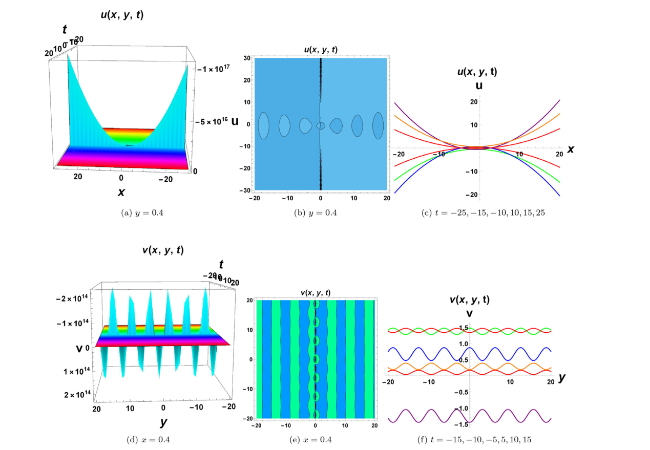
Fig. 1. Solitary wave form for Eq. (36). Figures (a), (d) indicate doubly soliton and multi soliton structures, (b), (e) represent corresponding contour plot while figures (c), (f) show wave propagation pattern. |
Figure 2 describe the multisoliton and kink behavior of wave component u and v for Eq. (43). This profile is plotted for a4=2, a5=200, a6=2.8, a=2.5, b=1.5 with range −20≤x, y≤20 and −20≤x, t≤20. As a result of simulation, it has been observed that existing waves behave differently based on y for wave component v. The wave’s energy is dissipated and the profile is annihilated into a stationary wave profile when y increases, whereas the wave component u does not change with the values of t. Complex multi-wave structures occur when more than one solution occurs in explicit solutions.
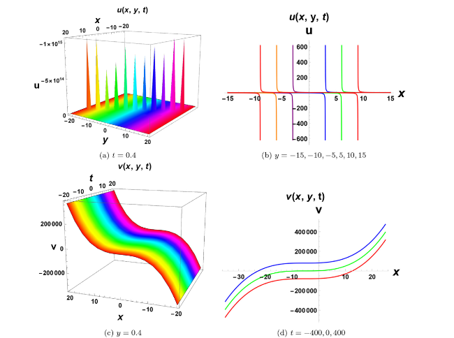
Fig. 2. Wave profile structures for Eq. (43). Figures (a), (c) exhibit singular-form and kink wave structures, while figures (b), (d) illustrate the propagation of waves along the x axis. |
Figure 3 describe the behavior of u(x, y) and v(x, y) in space x and y, which represents the singularity form and doubly soliton structure for Eq. (65). Plotting is done at ${{f}_{1}}\left( t \right)=sin\left( t \right)+cos\left( t \right)$, ${{f}_{2}}\left( t \right)=sin\left( t \right)+cos\left( t \right)$, a10=0.2, a11=2.3 with range −20≤x, y≤20. Variation in time affects the behavior of exiting wave. As t increases, the wave loses energy and start dissipating, destroying its profile into stationary form. Corresponding wave propagation pattern is shown along x-axis for wave component u and v at t=−25,−15,−10,10,15,25. This t−v view illustrates the elastic interaction property with high peaks.
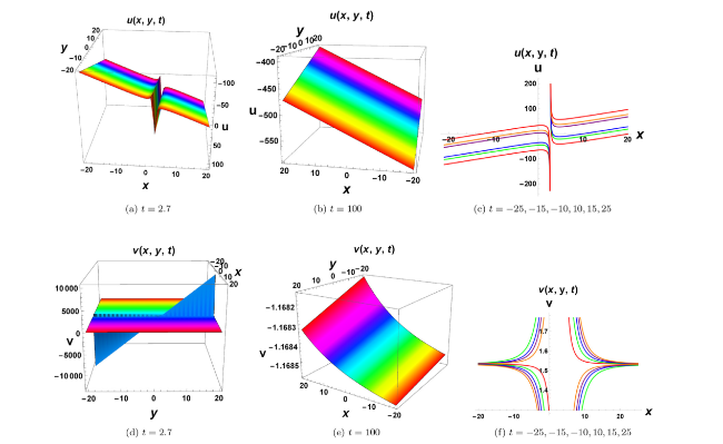
Fig. 3. Annihilation of solitary wave form for Eq. (65). Figures (a), (d) reveal singularity form and soliton structures, (b), (e) represent corresponding annihilation while figures (c), (f) show wave propagation pattern along x axis. |
Figure 4 display 2D and 3D plot of Eq. (77), which is a multisoliton solution and plotted when a13=2, a14=200, a15=2.8, a=2.5, b=1.5 with space range −20≤x, y≤20. We can observe that the shape of solitons remains stationary for wave component u with the change in the values of t while wave structure for v gets annihilate into kink wave as t increases. Two-dimensional illustrations show the propagation of the wave at y=−15,−10,−5,5,10,15 along x-axis. A slow decay in energy is shown with the influence of time for v.
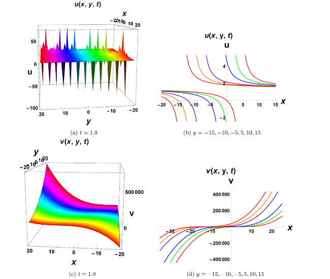
Fig. 4. Wave profile structures for Eq. (77). Figures (a), (c) exhibit multisoliton and wave structures, while figures (b), (d) represent wave propagation along x axis. |
Figure 5 represent 2D, 3D and contour plot of Eq. (85), which is a singularity form structure and plotted when a16=2.1, a17=1.2, ${{f}_{2}}\left( t \right)=sin\left( t \right)$ with −20≤x, t≤20. It was noted that nonlinearity of u and v ceases as y passes over 60. Dromion annihilation of wave structure reveals that the nonlinear behavior of the wave is overcome by the dissipation and is independent of choice of arbitrary constants.
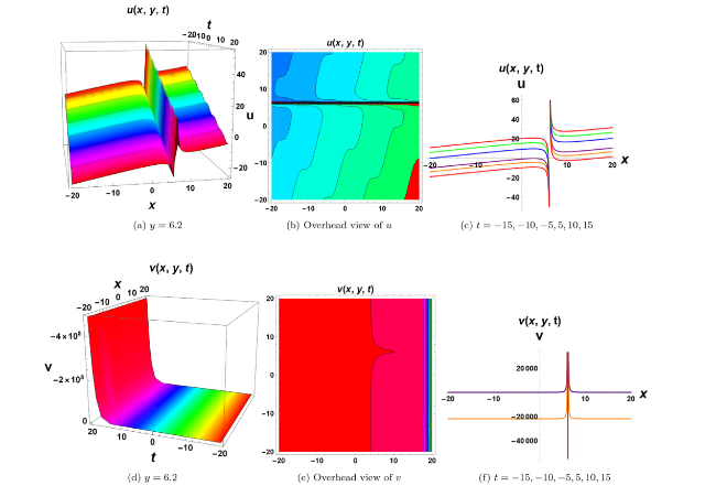
Fig. 5. Singular wave-form structure for Eq. (85). Figures (a), (d) display various wave structures, (b), (e) represent corresponding contour plot while figures (c), (f) illustrate the propagation of waves along the x axis. |
6. Conclusion
In this study, we investigated the new kink wave, singular wave profiles, and solitary wave solutions of the weakly coupled B-Type Kadomtsev-Petviashvili equation proposed in [59] by a well-organized Lie classical method. Eight fundamental symmetry algebras contain geometrical symmetry, and an optimal system of subalgebras is established for Eq. (3). Furthermore, by employing these subalgebras, the governing equation is reduced to new equations with fewer variables, allowing them to be solved analytically. The invariance property allows for systematic Lie symmetry reductions, leading to exact closed-form solutions of the governing system. Some new exact solutions are presented in their general forms as a result of this study. Due to the existence of arbitrary independent functional parameters and constants, these solutions have never been described in the literature and are more general than previous findings. We exhibited two- and three-dimensional wave profiles as well as some contour graphics to better comprehend the physical properties of the obtained solutions. Accordingly, wave-wave interactions, stripe soliton, single soliton, multi-peak solitons, soliton splitting, and the elastic structures of solitons are well-presented. As a result, the Lie symmetry method can be thought of as a powerful, robust, and versatile mathematical approach for finding analytical solutions to nonlinear PDEs. The applicability and relevance of the proposed approach are confirmed using illustrative approaches.
6.1. Future scope
Some of the obtained soliton solutions have various applications in mathematical physics, plasma physics, ocean engineering, solitons dynamics, and a wide range of other nonlinear sciences and engineering physics. As a result, in the future, the dynamics of various soliton solutions will provide an overarching theory to describe the experience of the complicated diversity in numerous nonlinear physical systems. Because the evolutionary behavior of soliton solutions has stimulated outstanding research and development in a wide range of fields, the potential benefits of interactions between shallow-water waves and the dynamical behavior of mixed solitons will be of great interest.
Declaration of Competing Interest
The authors declare that they have no conflict of interest.
Acknowledgments
The author, Sachin Kumar, wishes to express his gratitude to the Institution of Eminence, University of Delhi, India, for supporting this research through the IoE programme under Faculty Research Programme (FRP) with Ref. No./IoE/2021/12/FRP.
