
1. Introduction
Marine magnetic detection is widely used in submarine geological surveying and mapping, submarine resource exploration, military monitoring, and other fields [6,7,19]. With the acceleration of the investigation and development of marine resources, the detection and location of submarine pipelines have become a necessary part of modern marine engineering. At present, the location information of some submarine pipelines is lost for various reasons. For example, the original submarine pipelines have no layout map, the layout map of submarine pipelines is missing, and the existing layout location of submarine pipelines is inaccurate. Moreover, given the impact of the marine environment, most of the submarine pipelines are buried on the seabed by sediment. For buried submarine pipelines, optical detection cannot be conducted, and the acoustic detection error is relatively large. However, magnetic detection technology is not affected by optical and acoustic underwater attenuation [15,1,3]. Therefore, in the detection and location of buried submarine pipelines, magnetic detection has high detection accuracy and good reliability.
As a typically weak magnetic anomaly target underwater, the magnetic anomaly in submarine pipelines can only be detected within a certain distance. Nowadays, a towfish [33,9] and an autonomous underwater vehicle (AUV) [5,23] are mainly applied as detection platforms equipped with magnetometers. A towfish is a towed detection platform, which is generally far away from the mother ship. It is greatly affected by waves and currents, has poor stability, is difficult to sail at constant altitude, and easily collides with seabed obstacles, thus resulting in damage and loss of magnetometers. Meanwhile, the AUV is an autonomous underwater detection platform. Its real-time detection is relatively poor, and it has difficulty providing an accurate location; hence, its poor performance has a certain impact on the target location, inversion, and recognition based on the magnetic field. A two-part towed platform can solve the problems of these detection platforms. A deep-sea towed platform has a wide range of applications in marine environment exploration, seabed mapping, and submarine pipeline detection. Generally, a deep-sea towed platform is divided into a one-part towed platform [2,24,25,29] and a two-part towed platform [18]. Given that the two-part towed platform could effectively reduce the interference of the mother ship motion on the towed vehicle and has a certain heaving compensation function, an increasing number of scholars have focused on the research on the two-part towed platform. Wu and Chwang [20], [21], [22] established a mathematical model of the two-part towed platform by using the finite difference method. On the basis of this model, a simulation and an experimental verification of the motion state of the secondary towed vehicle were carried out. In addition, Lalu [10,11] established a mathematical model of a towed cable using the lumped mass method; combined with the CFD method, the influence of hydrodynamic coefficients on the motion state of a secondary towed vehicle was analyzed. However, none of the above scholars studied the active control of the secondary towed vehicle. Schuch [16,17] and Linklater [13] established the “spring-damping” model of the towed platform and examined the active control of the secondary towed vehicle. However, constant altitude sailing did not draw special attention. In short, the current two-part towed platform lacks the constant altitude sailing ability, which directly influences the detection effect of high-precision magnetic detection equipment. Therefore, the magnetic detection of submarine pipelines needs a platform that can sail at constant altitude on the seabed. Moreover, it must be equipped with magnetometers to approach the target.
To solve the problem regarding the magnetic detection of submarine pipelines, we constructed a magnetic detection system for submarine pipelines with constant altitude sailing ability based on a two-part towed platform. In this study, the mathematical model of the two-part towed platform was established, including the spring-damping model of the secondary towed cable and the kinematic and dynamic model of the secondary towed vehicle. Considering the strong nonlinearity and time-varying characteristics of the platform, a self-adaptive fuzzy PID controller was designed for the constant altitude sailing of the two-part towed platform. Then, according to the magnetic anomaly detection theory of submarine pipelines, the magnetic anomaly model of submarine pipelines was established. The magnetic anomaly of submarine pipelines was calculated theoretically, and the magnetic detection array on the two-part towed platform was designed. Finally, the experimental verification of the magnetic detection system of submarine pipelines was conducted.
2. Construction of magnetic detection system of submarine pipelines based on a two-part towed platform
2.1. Two-part towed platform
The two-part towed platform used in this study draws on Schuch's [17] two-part towed platform. The platform consists of the primary towed vehicle, the secondary towed vehicle, and the secondary towed cable, as shown in Fig. 1. The secondary towed vehicle draws on Teixeira's [18] secondary towed vehicle, which contains a horizontal bow and stern rudders, with the function of adjusting the altitude and attitude automatically. Teixeira's secondary towed vehicle is shown in Fig. 2. At the same time, an effective “spring-damping” model of the secondary towed cable is established, which can transmit external disturbance coming from the mother ship and surface jamming to the secondary towed vehicle without attenuation.
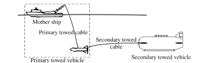
Fig. 1. Composition of the two-part towed platform. |
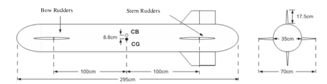
Fig. 2. Physical dimensions of the Teixeira's secondary towed vehicle. |
2.1.1. Mathematical model of the two-part towed platform
2.1.1.1. (1) spring-damping model of the secondary towed cable
In this model, the towed cable between the primary towed vehicle and the secondary towed vehicle could be simplified into a linear “spring-damping” model [17]. The motion of the primary towed vehicle is simplified to the motion state of the mother ship, and the simplified model is shown in Fig. 3. The spring coefficient is $\bar{k}$, as shown in Eq. (1).
$\bar{k}=\frac{E{{A}_{c}}}{L},$
where E is the elastic modulus of the secondary towed cable, ${{A}_{c}}$ is the cross-sectional area, and L is the length of the cable.

Fig. 3. Spring-damping model of secondary towed cable. |
2.1.1.2. (2) Kinematic and dynamic model of the secondary towed vehicle
The coordinate system of the towed vehicle system is established, which includes the body-fixed reference frame and the North-East-Down (NED) coordinate system [8]. In the NED system, the position and Euler angles are $\text{X}=\left[ x,y,z \right]$ and $\mathbf{\Phi }={{\left[ \phi,\theta,\psi \right]}^{T}}$, respectively, where ϕ is the rotation about the x axis (roll), θ is the rotation about the y axis (pitch), and ψ is the rotation about the z axis (yaw). The velocity and angular velocity of the towed vehicle are $\mathbf{\upsilon }={{\left[ u,v,w \right]}^{T}}$ and $\mathbf{\omega }={{\left[ p,q,r \right]}^{T}}$, respectively. The motion equation of the towed vehicle is Eq. (2).
$\left( \begin{matrix} {\dot{X}} \\ {\dot{\Phi }} \\\end{matrix} \right)=\left( \begin{matrix} {{J}_{1}}\left( \phi,\theta,\psi \right)\mathbf{\upsilon } \\ {{J}_{2}}\left( \phi,\theta \right)\mathbf{\omega } \\\end{matrix} \right),$
Where
$\begin{matrix} {} & {{J}_{1}}= \\ {} & \left( \begin{matrix} \cos \psi \cos \theta & -\sin \psi \cos \theta +\cos \psi \sin \theta \sin \phi & \sin \psi \sin \phi +\cos \psi \cos \phi \sin \theta \\ \sin \psi \cos \theta & \cos \psi \cos \phi +\sin \phi \sin \theta \sin \psi & -\cos \psi \sin \phi +\sin \theta \sin \psi \sin \phi \\ -\sin \theta & \cos \theta \sin \phi & \cos \theta \cos \phi \\ \end{matrix} \right), \\ {} & {{J}_{2}}=\left( \begin{matrix} 1 & \sin \phi \tan \theta & \cos \phi \tan \theta \\ 0 & \cos \phi & -\sin \phi \\ 0 & \frac{\sin \phi }{\cos \theta } & \frac{\cos \phi }{\cos \theta } \\ \end{matrix} \right). \\ \end{matrix}$
To determine the dynamical equation, the six degrees freedom of the inertia matrix of the towed vehicle is Eq. (3).
$\mathbf{\Gamma }=\left( \begin{matrix} M & {{D}^{T}} \\ D & J \\\end{matrix} \right),$
where M is the matrix of the mass and the added mass; J is the matrix of the inertia and the added inertia; D is the matrix of the hydrodynamic coupling matrix. The towed vehicle is assumed to be moving in an ideal fluid (water) in an infinite volume, and the relationship between linear momentum and angular momentum is Eq. (4).
$\begin{matrix} {} & {} & P\left( v,w \right)=Mv+{{D}^{T}}w, \\ {} & {} & \mathbf{\Pi }\left( v,w \right)=Jw+Dv. \\\end{matrix}$
Then, the dynamical equation is Eq. (5).
$\left( \begin{matrix} {\dot{v}} \\ {\dot{w}} \\ \end{matrix} \right)={{\text{ }\!\!\Gamma\!\!\text{ }}^{-1}}\left( \begin{matrix} P\left( v,w \right)\times w+{{F}_{ext}} \\ \mathbf{\Pi }\left( v,w \right)\times w+P\left( v,w \right)\times w+{{M}_{ext}} \\ \end{matrix} \right),$
where the external force is ${{F}_{ext}}={{F}_{body}}+{{F}_{rudder}}+{{F}_{towing}}+{{F}_{gravity}}+{{F}_{buoyancy}}$ and the external moment is ${{M}_{ext}}={{M}_{body}}+{{M}_{rudder}}+{{M}_{towing}}+{{M}_{gravity}}+{{M}_{buoyancy}}$.
1) Inertia force (${{F}_{body}}$) and moment (${{M}_{body}}$) of the towed vehicle
${{F}_{body}}={{R}_{BC}}\left( \left[ \begin{matrix} -{{C}_{D\alpha b}}{{\mu }^{2}}+{{C}_{D0}} \\ -\left( {{C}_{L\alpha b1}}\beta +{{C}_{L\alpha b2}}{{\beta }^{2}} \right) \\ -\left( {{C}_{L\alpha b1}}\alpha +{{C}_{L\alpha b2}}{{\alpha }^{2}} \right) \\ \end{matrix} \right]\bar{q}Vo{{l}^{2/3}}+\left[ \begin{matrix} -{{C}_{Db0}} \\ 0 \\ 0 \\ \end{matrix} \right]\bar{q}{{S}_{b}} \right),$
${{M}_{body}}=\left[ \begin{matrix} 0 \\ {{C}_{m\alpha b}}\alpha \\ -{{C}_{m\alpha b}}\beta \\ \end{matrix} \right]\bar{q}Vol,$
as shown in Eqs. (6) and (7),
where $\bar{q}=1/2{{\left| V \right|}^{2}}$, $Vol$ is the body volume, V is the towing velocity; Sb is the cross-section area, and ${{S}_{b}}=\mathbf{\pi }d_{b}^{2}/4$, db is the body diameter;
${{R}_{BC}}=\left[ \begin{matrix} \cos \alpha \cos \beta & -\cos \alpha \sin \beta & -\sin \alpha \\ \sin \beta & \cos \beta & 0 \\ \cos \beta \sin \alpha & -\sin \alpha \sin \beta & \cos \alpha \\\end{matrix} \right]$, which is the transfer matrix from the flow coordinate system to the body-fixed coordinate system; α, β, and μ are the hydrodynamic angles, which represent the angles between the resultant hydrodynamic force and the three axes of the body-fixed coordinate system, where α is the angle between the resultant hydrodynamic force and the x axis, β is the angle between the resultant hydrodynamic force and the y axis, and μ is the angle between the resultant hydrodynamic force and the z axis; ${{C}_{D\alpha b}},{{C}_{D0}}$ and ${{C}_{Db0}}$ are the drag coefficients; ${{C}_{L\alpha b1}}$ and ${{C}_{L\alpha b2}}$ are the lift coefficients; ${{C}_{m\alpha b}}$ is the pitching moment coefficient.
2) Force (${{F}_{rudder}}$) and moment (${{M}_{rudder}}$) of stern rudders
Forces generated by rudders include lift force, induced drag, and lateral force, in which the lift force and the induced drag are generated by horizontal stern rudders and the lateral force is generated by the vertical stern rudder. The force and moment are Eqs. (8) and (9).
${{F}_{rudder}}={{R}_{BC}}\left( 2{{C}_{vf}}+{{C}_{spl}}+{{C}_{spr}} \right)\frac{1}{2}{{S}_{f}}\bar{q},$
${{M}_{rudder}}=\frac{1}{2}{{S}_{f}}\bar{q}\left( {{\mathbf{X}}_{ac1}}{{R}_{BC}}{{C}_{vf}}+{{\mathbf{X}}_{ac2}}{{R}_{BC}}{{C}_{vf}}+{{\mathbf{X}}_{ac3}}{{R}_{BC}}{{C}_{spl}}+{{\mathbf{X}}_{ac4}}{{R}_{BC}}{{C}_{spr}} \right),$
where ${{S}_{f}}$ is the area of the horizontal and vertical rudders; ${{C}_{vf}}$ is the coefficient of the lateral force; ${{C}_{spl}}$ and ${{C}_{spr}}$ are the lift coefficients of the horizontal left and right stern rudders. ${{\mathbf{X}}_{ac1}},{{\mathbf{X}}_{ac2}},{{\mathbf{X}}_{ac3}}$ and ${{\mathbf{X}}_{ac4}}$ are the distance matrices from the hydrodynamic center of No.1, No.2, No.3, and No.4 rudder to the center line of the towed vehicle, respectively.
3) Towing force (${{F}_{towing}}$) and towing force moment (${{M}_{towing}}$)
After simplifying the secondary towed cable to the “spring-damping” model, the errors of the distance and velocity between the primary and secondary towed vehicles are Eqs. (10) and (11).
$\text{ }\!\!\Delta\!\!\text{ }x={{X}_{\text{primary}}}-\left( {{X}_{Initial}}+{{J}_{1}}\left| \begin{matrix} \frac{{{l}_{b}}}{2} \\ 0 \\ 0 \\\end{matrix} \right| \right),$
$\text{ }\!\!\Delta\!\!\text{ }u={{U}_{\text{primary}}}-\left( {{J}_{1}}V+{{J}_{1}}\left( \mathbf{\Omega }\times \left| \begin{matrix} \frac{{{l}_{b}}}{2} \\ 0 \\ 0 \\\end{matrix} \right| \right) \right),$
where ${{X}_{\text{primary}}}$ and ${{U}_{\text{primary}}}$ are the position and velocity of the primary towed vehicle, respectively; ${{X}_{Initial}}$ is the initial position of the secondary towed vehicle; ${{l}_{b}}$ is the length of the secondary towed vehicle. ${{J}_{1}}$ is the rotation matrix from the box-fixed frame to the NED frame. Ω is the angle velocity of the secondary towed vehicle in the body-fixed frame.
In the inertial frame, the towing force is Eq. (12).
${{\mathbf{F}}_{td}}=\left[ \begin{matrix} \bar{k}\left( \left| \text{ }\!\!\Delta\!\!\text{ }x-L \right| \right)+\bar{b}\left( \left( \text{ }\!\!\Delta\!\!\text{ }u\cdot \frac{\text{ }\!\!\Delta\!\!\text{ }x}{\left| \text{ }\!\!\Delta\!\!\text{ }x \right|} \right) \right) \\ 0 \\ 0 \\\end{matrix} \right],$
where $\bar{k}$ is the spring constant, L is the length of the secondary towed cable and $\bar{b}$ is the damping coefficient.
To transfer the towing force from the inertial frame to the box-fixed coordinate system, a transfer matrix ${{R}_{IT}}$ is needed, which is
${{R}_{IT}}=\left[ \begin{matrix} \cos \gamma \cos \sigma & -\cos \gamma \sin \sigma & -\sin \gamma \\ \sin \sigma & \cos \sigma & 0 \\ \cos \sigma \sin \gamma & -\sin \gamma \sin \sigma & \cos \gamma \\\end{matrix} \right],$
In Eq. (13), attack angle γ and drift angle σ are shown in the following figure (Fig. 4).

Fig. 4. Towing angle for the towing force. |
Then, the towing force and moment of the secondary towed vehicle are obtained, as shown in Eqs. (14) and (15):
$\ {{\mathbf{F}}_{tow}}=\{\begin{matrix} {{J}_{1}}^{T}{{R}_{IT}}{{F}_{td}} & \left| \text{ }\!\!\Delta\!\!\text{ }x \right|>L \\ 0 & \left| \text{ }\!\!\Delta\!\!\text{ }x \right|\le L \\\end{matrix},$
${{M}_{tow}}={{\left[ \begin{matrix} \frac{{{l}_{b}}}{2} & 0 & 0 \\\end{matrix} \right]}^{T}}\cdot {{F}_{tow}}.$
4) Gravity (${{F}_{gravity}}$) and gravitational moment (${{M}_{gravity}}$)
${{F}_{\text{gravity}}}={{J}_{1}}^{T}\left[ \begin{matrix} 0 \\ 0 \\ {{W}_{b}} \\\end{matrix} \right],$
${{M}_{\text{gravity}}}={{X}_{CG}}\cdot {{F}_{gravity}},$
as shown in Eqs. (16) and (17),
where ${{X}_{CG}}$ is the offset of the center of gravity with respect to the buoyancy center and ${{W}_{b}}$ is the weight of the secondary towed vehicle.
5) Buoyancy and buoyancy momentAs shown in Eqs. (18) and (19),
${{F}_{\text{buoyancy}}}=-\left( 1.05 \right){{J}_{1}}^{T}\left[ \begin{matrix} 0 \\ 0 \\ {{W}_{b}} \\\end{matrix} \right],$
${{M}_{\text{buoyancy}}}=0.$
2.1.2. Constant altitude sailing study of the two-part towed platform
2.1.2.3. (1) Controller designing of the secondary towed vehicle
The secondary towed vehicle can be easily disturbed by the attitude of the towing mother ship and the external environment, such as wind, wave, and current in the working process. Moreover, the platform is strong nonlinear and time-varying [27]. A conventional proportion integration differentiation (PID) controller has good control effect on linear systems. However, for a relatively complex two-part towed platform, it may not work properly. The parameters of the PID controller must be different under different working conditions and environments, that is, have a parameter self-adaptive function.
The fuzzy control rules are used in this study to correct the PID parameters online automatically to form a self-adaptive fuzzy strategy. The self-adaptive fuzzy PID controller [34,32,4] not only has a simple principle, convenient use, and strong robustness, but it also has high flexibility and stability. To ensure the accuracy of the measurement data of magnetometers equipped on the secondary towed vehicle, the vehicle needs to maintain the altitude and attitude stability by autonomously adjusting the horizontal bow and the stern rudders (maximum stroke is ± 45°) during the towing process. The mother ship is in a straight course, and the yaw angle of the body remains unchanged. Notably, relevant studies [22,11] have shown that a change in the roll angle is very small or could even be neglected, that is, only the pitch angle change is considered. Therefore, the design goal of the controller is that the towed vehicle can reach a steady state through self-adjustment in a short time when the sea state changes. When the sea state is at its worst, the pitch angle can vary within ± 5° In addition, the altitude variation is between ± 0.5 m, while the angle changes of the horizontal bow and stern rudders are within ± 45°
2.1.2.4. (2) Principle and structure of the self-adaptive fuzzy PID controller
The structure of the self-adaptive fuzzy PID controller is mainly composed of two parts: the parameter adjustable PID part and the fuzzy control part, as shown in Fig. 5.
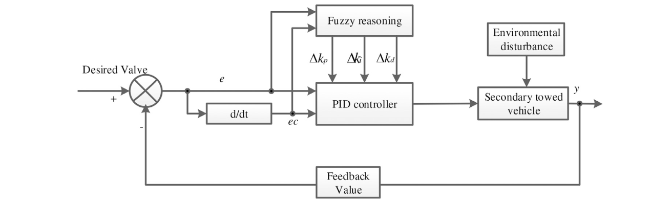
Fig. 5. Structure of self-adaptive fuzzy PID controller. |
Taking the error e and the change rate of error ec as inputs, fuzzy inference uses fuzzy rules to adjust the PID parameters in real time to satisfy the different requirements of controller parameters under different e and ec.
2.1.2.5. (3) Designing the self-adaptive fuzzy PID controller
According to the design requirements, the fuzzy controller used for PID parameter adjustment adopts two inputs and three outputs. The controller takes the error e and ec as inputs and the three corrected parameters $\text{ }\!\!\Delta\!\!\text{ }{{k}_{p}}$, $\text{ }\!\!\Delta\!\!\text{ }{{k}_{i}}$, and $\text{ }\!\!\Delta\!\!\text{ }{{k}_{d}}$ of the PID controller as outputs. The fuzzy domain for e, ec, $\text{ }\!\!\Delta\!\!\text{ }{{k}_{p}}$, $\text{ }\!\!\Delta\!\!\text{ }{{k}_{i}}$, and $\text{ }\!\!\Delta\!\!\text{ }{{k}_{d}}$ is {NB, NM, NS, ZO, PS, PM, PB}. According to the actual needs and referring to relevant experience, the basic domain for depth error e is [−0.5 m, 0.5 m], the basic domain for change of rate ec is [−0.1 m/s, 0.1 m/s], and the fuzzy domain is {−0.3, −0.2, −0.1, 0, 0.1, 0.2, 0.3}. For the pitch error, the basic domain of e is [−5°, 5°], ec is [−2∘/s, 2∘/s], and the fuzzy domain is {−3, −2, −1, 0, 1, 2, 3}.
According to the membership degree and fuzzy control model of each fuzzy subset, fuzzy reasoning is applied to design the fuzzy matrix table of the PID parameters. The parameters are calculated using the following formula Eq. (20):
$\left\{\begin{array}{l} k_{p}=k_{p 0}+\Delta k_{p} \\ k_{i}=k_{i 0}+\Delta k_{i} \\ k_{d}=k_{d 0}+\Delta k_{d} \end{array}\right. $
Where ${{k}_{p0}}$, ${{k}_{i0}}$, and ${{k}_{d0}}$ are the initial parameter values, which are designed using the conventional PID controller. $\text{ }\!\!\Delta\!\!\text{ }{{k}_{p}}$, $\text{ }\!\!\Delta\!\!\text{ }{{k}_{i}}$, and $\text{ }\!\!\Delta\!\!\text{ }{{k}_{d}}$ are the outputs of the fuzzy controller. According to the state of the controlled object, three PID controller parameters can be adjusted automatically. The fuzzy rule of $\text{ }\!\!\Delta\!\!\text{ }{{k}_{p}}$, $\text{ }\!\!\Delta\!\!\text{ }{{k}_{i}}$ and $\text{ }\!\!\Delta\!\!\text{ }{{k}_{d}}$ is shown in Table 1.
Table 1. Fuzzy rule of $\text{ }\!\!\Delta\!\!\text{ }{{k}_{p}}$, $\text{ }\!\!\Delta\!\!\text{ }{{k}_{i}}$, $\text{ }\!\!\Delta\!\!\text{ }{{k}_{d}}$. |
| KP,KI,KD | E | |||||||
|---|---|---|---|---|---|---|---|---|
| NB | NM | NS | ZO | PS | PM | PB | ||
| EC | NB | PB,ZO,PS | PB,PS,PS | PM,PB,PM | PS,PB,PB | PM,PB,PM | PB,PS,PS | PB,ZO,PS |
| NM | PB,ZO,PS | PB,PS,PS | PM,PB,PM | PS,PB,PB | PM,PB,PM | PB,PS,PS | PB,ZO,PS | |
| NS | PB,ZO,PS | PM,ZO,PM | PS,PM,PB | ZO,PB,PB | PS,PM,PB | PM,ZO,PM | PB,ZO,PS | |
| ZO | PB,ZO,PS | PM,ZO,PM | PS,PM,PB | ZO,PB,PB | PS,PM,PB | PM,ZO,PM | PB,ZO,PS | |
| PS | PB,ZO,PS | PM,ZO,PM | PS,PM,PB | ZO,PB,PB | PS,PM,PB | PM,ZO,PM | PB,ZO,PS | |
| PM | PB,ZO,PS | PM,PS,PS | PM,PB,PM | PS,PB,PB | PM,PB,PM | PB,PB,PS | PB,ZO,PS | |
| PB | PB,ZO,PS | PM,PS,PS | PM,PB,PM | PS,PB,PB | PM,PB,PM | PB,PS,PS | PB,ZO,PS | |
2.2. Research on magnetic anomaly detection theory and magnetic detection array of submarine pipelines
2.2.1. Magnetic anomaly model of submarine pipelines
Owing to the surroundings of submarine pipelines and the complexity of the structure, the pipelines can be equivalent to 2D infinite-length horizontal cylinders [31,28]. The theory of the 2D infinite-length model of a horizontal cylinder is widely used in studies on the magnetic field model of submarine pipelines or cables [26,14,30,19]. The basic idea of the theory is to approximate submarine pipelines or cables to 2D infinite-length horizontal cylinders to analyze their magnetic field.
According to the literature [31] (P90), the total intensity magnetic anomaly of any form can be expressed as follows Eq. (21):
$\text{ }\!\!\Delta\!\!\text{ }T={{H}_{\text{ax}}}\cos I\cos {A}'+{{H}_{ay}}\cos I\sin {A}'+{{Z}_{a}}\sin I,$
where ΔT is the total intensity magnetic anomaly, I is the magnetization dip angle, ${A}'$ is the angle between the cross section of the submarine pipeline and magnetic north, and ${{H}_{ax}},{{H}_{ay}},{{Z}_{a}}$ are the three components of the magnetic field.
On the basis of the Poisson Formula between the magnetic potential and the gravitational potential [31] (P95),
$\begin{matrix} U & =-\frac{1}{4\pi G\sigma }\vec{M}\cdot \nabla \vec{V}, \\ {{H}_{ax}} & =\frac{{{\mu }_{0}}}{4\pi G\sigma }\left[ {{M}_{x}}{{V}_{xx}}+{{M}_{y}}{{V}_{yx}}+{{M}_{z}}{{V}_{zx}} \right], \\ {{H}_{ay}} & =\frac{{{\mu }_{0}}}{4\pi G\sigma }\left[ {{M}_{x}}{{V}_{xy}}+{{M}_{y}}{{V}_{yy}}+{{M}_{z}}{{V}_{zy}} \right], \\ {{Z}_{a}} & =\frac{{{\mu }_{0}}}{4\pi G\sigma }\left[ {{M}_{x}}{{V}_{xz}}+{{M}_{y}}{{V}_{yz}}+{{M}_{z}}{{V}_{zz}} \right]. \\ \end{matrix}$
where G is the gravitational constant, σ is the density of the cylinder, $\vec{M}$ is the total magnetization vector, and $\vec{V}$ is the gravitational potential vector.
A magnetic body is 2D when it extends infinitely along the strike direction; the burial depth, the shape of the cross section, the size, and the magnetization characteristics of the magnetic body are stable in the same direction [31] (P90). When a horizontal cylinder is extended infinitely along the strike direction and its burial depth, cross-section shape, and magnetization characteristics are stable in the same direction, the horizontal cylinder is a 2D infinite-length horizontal cylinder. The total intensity magnetic anomaly of a 2D infinite-length horizontal cylinder in a rectangular coordinate system is related to (x, z) but not to y [31] (P105), as shown in Eq. (23).
$\text{ }\!\!\Delta\!\!\text{ }T={{H}_{\text{ax}}}\cos I\cos {A}'+{{Z}_{a}}\sin I.$
At this time, the Poisson formula Eq. (22) of the 2D infinite-length horizontal cylinder in the rectangular coordinate system becomes Eq. (24) [31] (P95):
$\begin{matrix} {{H}_{ax}} & =\frac{{{\mu }_{0}}}{4\pi G\sigma }\left[ {{M}_{x}}{{V}_{xx}}+{{M}_{z}}{{V}_{zx}} \right], \\ {{H}_{ay}} & =0, \\ {{Z}_{a}} & =\frac{{{\mu }_{0}}}{4\pi G\sigma }\left[ {{M}_{x}}{{V}_{xz}}+{{M}_{z}}{{V}_{zz}} \right]. \\ \end{matrix}$
In light of field theory, the gravitational potential of the infinite horizontal cylinder is Eq. (25).
$V=-2G\sigma S\ln r,$
where S is the cross-sectional area of the cylinder; r is the distance from the observation point to the cylinder axis.
The magnetic anomaly model of the 2D infinite-length horizontal cylinder is shown in Fig. 6. P(x, y, z) is the observation point, and Q(ξ, η, ζ) is the projection of point P on the cylinder axis. Thus, $r=|\overrightarrow{PQ}|$, η = y and as shown in Eq. (26),
$r={{\left[ {{\left( x-\xi \right)}^{2}}+{{\left( z-\zeta \right)}^{2}} \right]}^{\frac{1}{2}}}.$
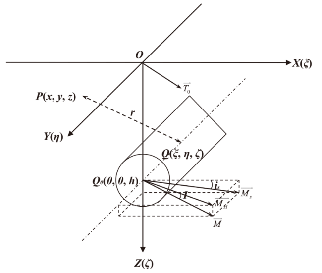
Fig. 6. Magnetic anomaly model of 2D infinite-length horizontal cylinder. |
$\overrightarrow{{{T}_{0}}}$ is the geomagnetic field, $\overrightarrow{{{M}_{H}}}$ is the projection of $\vec{M}$ on the horizontal plain (XOY), $\overrightarrow{{{M}_{s}}}$ is the effective magnetization vector, and ${{i}_{s}}$ is the effective magnetization dip angle.
If the Y-axis of the selected coordinate system is the projection of the cylinder axis on the ground plane (XOY), then ξ= 0, ζ= h, and z = 0. When the magnetization of submarine pipelines ($\vec{M}$) is consistent with the direction of the geomagnetic field ($\overrightarrow{{{T}_{0}}}$), the total intensity magnetic anomaly of submarine pipelines in the geomagnetic background field can be obtained:
$\text{ }\!\!\Delta\!\!\text{ }T=\frac{{{\mu }_{0}}{{M}_{s}}S}{2\pi {{\left( {{x}^{2}}+{{h}^{2}} \right)}^{2}}}\bullet \frac{\sin I}{\sin {{i}_{s}}}\left[ \left( {{h}^{2}}-{{x}^{2}} \right)\sin \left( 2{{i}_{s}}-{{90}^{\circ }} \right)-2hx\cos \left( 2{{i}_{s}}-{{90}^{\circ }} \right) \right],$
where μ0 is the vacuum permeability; h is the depth of the cylinder axis.
2.2.2. Theoretical calculation of magnetic anomaly of submarine pipelines
According to the magnetic anomaly model of submarine pipelines, the magnetic anomaly of submarine pipelines is calculated theoretically. Considering Eq. (27) and Fig. 6, Eq. (28) can be obtained.
$\begin{matrix} \frac{\sin I}{\sin {{i}_{s}}}=\frac{\left| \overrightarrow{{{M}_{S}}} \right|}{\left| {\vec{M}} \right|}\le 1, \\ \Rightarrow 0\le I\le {{i}_{s}}\le \pi -I\le \pi. \\\end{matrix}$
Without loss of generality, the effective magnetization of submarine pipelines is set as Ms = 1000 A/m, the distance range in X direction is [−50 m, 50 m], the magnetization dip angle is I = 45°, the axis depth of submarine pipelines is h = 2 m, the outer diameter of submarine pipelines is 21 mm, and the equivalent cross-sectional area of submarine pipelines is S = 1385.4424 × 10−6 m2 [28].
2.2.2.6. (1) When the magnetization dip angle = effective magnetization dip angle
At this time, I = ${{i}_{s}}$; the theoretical calculation results of the magnetic anomaly of submarine pipelines at different effective magnetization dip angles [150°] are shown in Fig. 7.
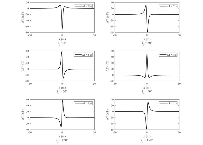
Fig. 7. Theoretical calculation results of magnetic anomaly of submarine pipelines when the magnetization dip angle is equal to the effective magnetization dip angle. |
According to Fig. 7, the magnetic anomaly of submarine pipelines is related to the effective magnetization dip angle is, which affects the magnetic anomaly waveform characteristics and magnetic field intensity of submarine pipelines.
2.2.2.7. (2) When magnetization dip angle ≠ effective magnetization dip angle
This moment assumes that I = 45°; the theoretical calculation results of the magnetic anomaly of submarine pipelines at different effective magnetization dip angles [60°, 75°, 90°, 105°, 120°, 135°] are shown in Fig. 8.
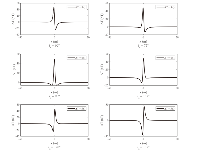
Fig. 8. Theoretical calculation results of magnetic anomaly of submarine pipelines when the magnetization dip angle is not equal to the effective magnetization dip angle. |
Fig. 8 indicates that the effective magnetization dip angle ${{i}_{s}}$ affects the magnetic anomaly waveform characteristics and magnetic field intensity of submarine pipelines. Compared with Fig. 7 Fig. 8, under the same effective magnetization dip angle ${{i}_{s}}$, the variation of the magnetization dip angle I only changes the magnetic anomaly in the magnetic field intensity of submarine pipelines and does not change the magnetic anomaly waveform characteristics of the pipelines.
2.2.3. Design of magnetic detection array
To reduce the interference of the two-part towed platform itself to magnetic detection, scalar magnetometers are considered the magnetic detection equipment. Compared with vector magnetometers, scalar magnetometers have the important advantage of being insensitive to rotational vibration. Therefore, they easily form an array without considering the orientation error, thus improving the detection accuracy of the array. Meanwhile, some types of scalar magnetometers, such as optical pump magnetometers and Overhauser magnetometers, also have high sensitivity. In this work, a magnetic detection array is designed on the basis of SeaQuest Overhauser magnetometers. The absolute accuracy of the magnetometers is 0.1 nT, the sensitivity is 0.01 nT, and the basic noise spectral density is 0.01 nT/√Hz. The magnetometers have sufficient accuracy to detect the magnetic anomaly of submarine pipelines.
Therefore, four scalar SeaQuest Overhauser magnetometers are used in this study to form a magnetic detection array for building the magnetic detection system. For the magnetic detection array, as shown in Fig. 9, four magnetometers are placed at points A, B, C, and D to form a rectangular array. Given that the magnetometers obtain the total magnetic field intensity T in real time, T0 is the geomagnetic field. In addition, T0 can be obtained through a separate measurement of the geomagnetic field, and the magnetic anomaly for the calculation can be obtained from ΔT = T - T0. Magnetic anomalies ΔT1, ΔT2, ΔT3, and ΔT4 are obtained by four magnetometers at points A, B, C, and D. The O-XYZ coordinate system is established through the horizontal plane, where the four magnetometers are located. On the XOY coordinate plane, the magnetometer coordinates are set to A(-t0, 0), B(t0, 0). t0 represents the distance between the magnetometer and the origin O, AD = BC = S; S represents the distance between A and D magnetometers and between B and C magnetometers. Then, the magnetometer coordinates are C(-t0, S), D(-t0, S). S and t0 are the array layout parameters. The parameter size can be adjusted according to the array detection requirements. After the array installation, the layout parameters are known and constant.

Fig. 9. Magnetic detection array. |
The magnetic detection array has the functions of magnetic anomaly detection and magnetic field location.
2.2.3.8. (1) Magnetic anomaly detection function
The two-part towed platform is equipped with the magnetic detection array. After the array is close to the target to be measured on the seabed, each magnetometer in the array will measure the magnetic field change curve under the influence of the target when passing directly above the target. The measured target magnetic field variation curve is compared with the theoretical curve of the magnetic anomaly of submarine pipelines. Without prior knowledge, the possibility of the target detected by magnetic anomaly can be inferred; with prior knowledge, the target of magnetic anomaly detection can be analyzed definitively. Finally, the function of magnetic anomaly detection can be realized.
2.2.3.9. (2) Magnetic field location function
After determining that submarine pipelines are the target to be measured on the seabed, the two-part towed platform is equipped with the magnetic detection array to ensure that the array is close to the submarine pipelines. In the array coordinate system, as shown in Fig. 9, the submarine pipeline to be measured is horizontally buried on the seabed, as expressed in MN. h (h > 1 m) is the depth from the submarine pipeline to the array. In addition, α is the included angle between the projection of the submarine pipeline on XOY coordinate plane and the Y axis. Meanwhile, E(0, -b) is the intersection of the submarine pipeline projection and the Y axis. The distances between the submarine pipeline and the four magnetometers are r1, r2, r3, and r4, which are unknown parameters.
According to magnetic field theory and array structure theory, the location of the submarine pipeline can be deduced and solved.
$\begin{matrix} \text{ }\!\!\Delta\!\!\text{ }{{T}_{1}} & =\frac{{{C}_{0}}}{{{h}^{2}}+{{\left( b\text{sin}\alpha +{{t}_{0}}\cos \alpha \right)}^{2}}}={{T}_{1}}-{{T}_{0}}, \\ \text{ }\!\!\Delta\!\!\text{ }{{T}_{2}} & =\frac{{{C}_{0}}}{{{h}^{2}}+{{\left( b\text{sin}\alpha -{{t}_{0}}\cos \alpha \right)}^{2}}}={{T}_{2}}-{{T}_{0}}, \\ \text{ }\!\!\Delta\!\!\text{ }{{T}_{3}} & =\frac{{{C}_{0}}}{{{h}^{2}}+{{\left[ \left( b+S \right)\text{sin}\alpha -{{t}_{0}}\cos \alpha \right]}^{2}}}={{T}_{3}}-{{T}_{0}}, \\ \text{ }\!\!\Delta\!\!\text{ }{{T}_{4}} & =\frac{{{C}_{0}}}{{{h}^{2}}+{{\left[ \left( b+S \right)\text{sin}\alpha +{{t}_{0}}\cos \alpha \right]}^{2}}}={{T}_{4}}-{{T}_{0}}. \\ \end{matrix}$
ΔT1, ΔT2, ΔT3, and ΔT4 are the magnetic anomalies measured by four magnetometers, all of which are known parameters. Meanwhile, S and t0 are both known array layout parameters. Thus, the four unknowns h, α, b, and C0 can be obtained by solving Eq. (29) through programming by Matlab.
According to h, α, b, and C0, the distance ro from the submarine pipeline to the origin O of the coordinate axis can be obtained as Eq. (30):
$r_{o}^{2}={{h}^{2}}+{{b}^{2}}{{\sin }^{2}}\alpha.$
Thus, the location of the submarine pipeline can be determined. The depth of the submarine pipeline is h, and the projection in the XOY coordinate plane can be expressed as Eq. (31):
$y=x\cot \alpha -b.$
Combined with the location information of the two-part towed platform, the actual location of the submarine pipeline can be calibrated to realize the magnetic field location function of the submarine pipeline.
3. Experimental verification of magnetic detection system for submarine pipelines
3.1. Verification of constant altitude sailing ability of the two-part towed platform
The constant altitude sailing ability of the two-part towed platform is verified by using the prototype of the magnetic detection system for submarine pipelines. The secondary towed vehicle in the platform of the system prototype is shown in Fig. 10. The main scale is approximately 3.0 × 1.8 × 1.2 m, the weight is approximately 0.7 t, and the main parameters of the secondary towed vehicle prototype are shown in Table 2. Meanwhile, the secondary towed vehicle is mainly made of aluminum and non-metallic materials and adopts a hydraulic horizontal bow and stern rudders for altitude and attitude control to minimize magnetic field interference. In the secondary towed vehicle prototype, the hydraulic horizontal bow and stern rudders are controlled by the self-adaptive fuzzy PID controller designed in Section 2.1.2.
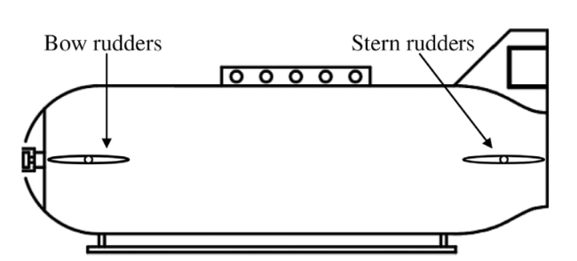
Fig. 10. Secondary towed vehicle prototype. |
Table 2. Main parameters of the secondary towed vehicle prototype. |
| Parameter | Value | Parameter | Value |
|---|---|---|---|
| L/m | 50 | V/(m·s − 1) | 2 |
| $E{{A}_{c}}$/(kN·m − 1) | 5.0000 | ${{C}_{L\alpha b1}}$ | 0.1858 |
| Vol/m3 | 0.2529 | ${{C}_{L\alpha b2}}$ | 0.9640 |
| Sb/m2 | 0.1464 | ${{C}_{m\alpha b}}$ | 1.3076 |
| ${{C}_{D\alpha b}}$ | 0.3511 | ${{l}_{b}}$/m | 2.9908 |
| ${{C}_{Db0}}$ | 0.0194 | ${{X}_{CG}}$/m | [0 0 0.0762] |
3.1.1. Hydrostatic constant altitude sailing experiment of the two-part towed platform
The hydrostatic constant altitude sailing experiment was carried out in the towing tank of Shanghai Jiao Tong University. In the experiment, the platform adopted the control strategy of parallel rudders for constant altitude sailing. The control altitude was set as 2 m with an error range of ± 0.5 m, and the pitch was 0° with an error range of ± 5° The stable stage of the platform was defined as that in which the altitude from the seabed to the secondary towed vehicle of the two-part towed platform was stable at 2 m, with an error within ± 0.5 m. The pitch was stable at 0° with a variation range within 5° The experiment results are as follows.
According to Fig. 11-Fig. 13 and Table 3, the secondary towed vehicle was released by the two-part towed platform and reached the set altitude in the adjustment stage. After that, the platform entered the stable stage. At this time, the altitude and pitch angle of the secondary towed vehicle remained stable. In addition, the parameters met the error range setting, and the variance was very small.
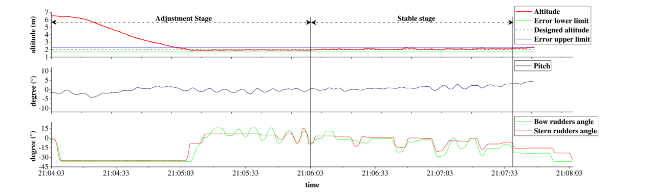
Fig. 11. Group 1 constant altitude experiment data. |
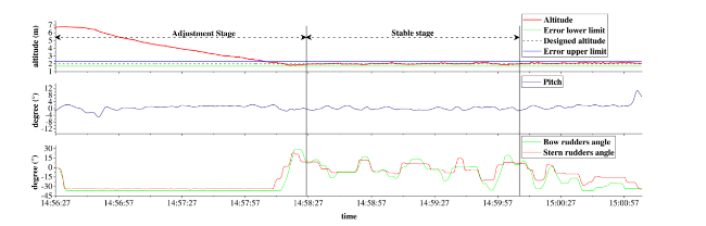
Fig. 12. Group 2 constant altitude experiment data. |

Fig. 13. Group 3 constant altitude experiment data. |
Table 3. Hydrostatic constant altitude sailing experiment results of the two-part towed platform. |
| Average altitude (m) | Altitude variance (m2) | Average pitch (°) | Pitch variance (°^2) | |
|---|---|---|---|---|
| Group 1 | 2.02 | 0.005 | 0.25 | 0.091 |
| Group 2 | 2.03 | 0.004 | 0.06 | 0.136 |
| Group 3 | 2.03 | 0.003 | 0.16 | 0.028 |
This outcome illustrates that the two-part towed platform has good constant altitude sailing ability in a hydrostatic environment.
3.1.2. Offshore constant altitude sailing experiment of the two-part towed platform
Table 4. Parameters of Sea States. |
| Sea State | 1 | 2 | 3 | 4 | 5 | 6 | 7 |
|---|---|---|---|---|---|---|---|
| Average wave height (m) | 0.05 | 0.3 | 0.88 | 1.88 | 3.25 | 5 | 7.5 |
Under the condition of low-speed towing of the mother ship, the control altitude was set as 2 m with an error of ± 0.5 m. Furthermore, the pitch angle was 0° with the error range ± 5° The changes of the secondary towed vehicle altitude, pitch angle, and angle of bow and stern rudders of the platform in the experiment are shown in Fig. 14.

Fig. 14. Offshore constant altitude sailing experiment data of the two-part towed platform. |
According to the information in Fig. 14 and Table 5, the secondary towed vehicle was released by the two-part towed platform and dove to an altitude of 3.45 m from the seabed to start the constant altitude sailing. Then, it entered the stable stage after approximately 50 s. At this time, the average altitude of the secondary towed vehicle was 1.89 m, the standard deviation of altitude was 0.11 m, the average pitch was 1.70°, and the standard deviation of pitch was 0.76°
Table 5. Offshore constant altitude sailing experiment results of the two-part towed platform. |
| Average | Standard deviation | Variation amplitude | |
|---|---|---|---|
| Altitude | 1.89 m | 0.11 m | 0.35 m |
| Pitch | 1.70° | 0.76° | 0.5° |
This outcome illustrates that the two-part towed platform also has good constant altitude sailing ability in the actual marine environment.
3.2. Functional verification of the magnetic detection system for submarine pipelines
Through the offshore magnetic anomaly detection experiment of submarine pipelines, the stable measurement function of the magnetic field and the function of the system to detect magnetic anomaly of these pipelines were verified. The experiment sea area was the same as that in Section 3.1.2. In the experiment, the two-part towed platform sailing at constant altitude vertically passed directly above the submarine pipeline with prior knowledge, as shown in Fig. 15. The secondary towed vehicle in the platform was equipped with a magnetic detection array (ABCD), and the total magnetic field (including background magnetic field, platform interference magnetic field, and the magnetic anomaly of the submarine pipeline) was measured by a single magnetometer in the array. The total magnetic field, background magnetic field, and theoretical magnetic anomaly of submarine pipelines were compared and analyzed to verify the function of the system.
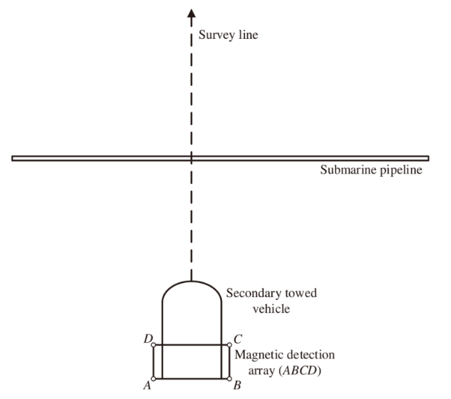
Fig. 15. Survey line of the offshore magnetic anomaly detection experiment of submarine pipelines. |
3.2.1. Functional verification of the stable measurement of the magnetic field
To verify the stable measurement function of the system for the magnetic field, the static geomagnetic field was used as the background magnetic field, which was compared with the total magnetic field measured in the offshore magnetic anomaly detection experiment. Therefore, a single scalar SeaQuest Overhauser magnetometer was used to measure the static geomagnetic field at three different positions in the experiment sea area, namely, position 1 (17°48′12″N, 110°01′06″E), position 2 (17°42′34″N, 109°59′54″E), and position 3 (17°36′56″N, 109°58′42″E). The static geomagnetic field measurement results are shown in Fig. 16.
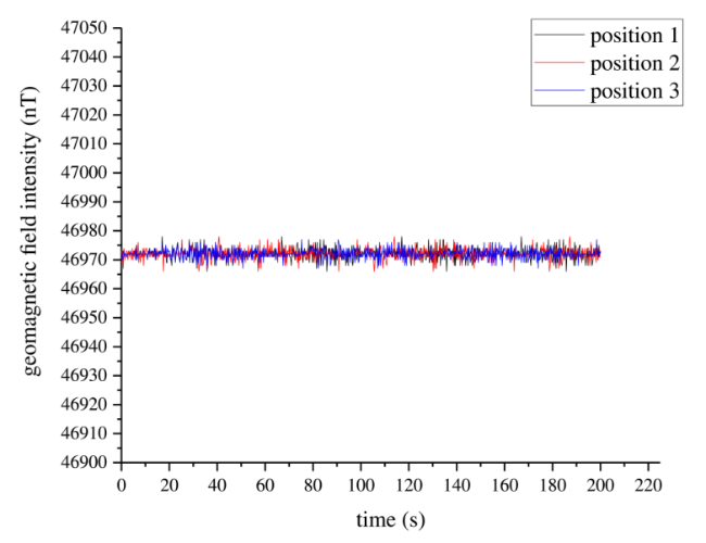
Fig. 16. Static geomagnetic field measurement results at different positions in the experiment sea area. |
According to Fig. 16, the static geomagnetic field intensity in the experiment sea area is approximately 46,973 nT, with a variation range of 3-5 nT. Considering the spatial and temporal variation law of geomagnetic field theory [31] (P1 ∼ P26), the average value of the static geomagnetic field measurement results at three positions was used as the background magnetic field of the offshore magnetic anomaly detection experiment.
On the basis of the comparison between the background magnetic field and the total magnetic field measured by the offshore magnetic anomaly detection experiment in Fig. 17, the whole submarine pipeline magnetic anomaly detection experiment was divided into three stages; 0-60 s (Stage 1) was the approaching target stage, 60-120 s (Stage 2) was the suspected target detection stage, and 120-180 s (Stage 3) was the far target stage. In Stage 1 and Stage 3, the two-part towed platform was far away from the suspected target, and the magnetic anomaly of the suspected target was small. The magnetometer in the magnetic detection array could not distinguish the magnetic anomaly of the suspected target from the total magnetic field measurement under the influence of the two-part towed platform sailing at constant altitude. At this time, the magnetic anomaly of the suspected target could be ignored. Therefore, theoretically, the total magnetic field measured in these two stages was the superposition of the background magnetic field and the platform interference magnetic field.
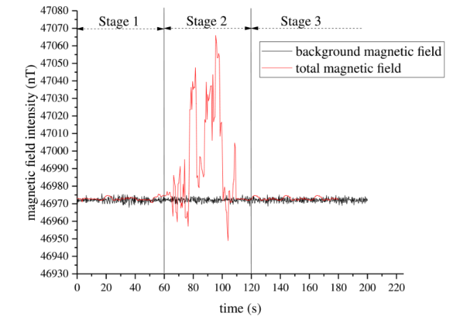
Fig. 17. Comparison between background magnetic field and total magnetic field measured by experiment. |
As shown in Fig. 17, the total magnetic field measured in Stage 1 and Stage 3 was basically the same as the background magnetic field. Thus, the interference magnetic field of the platform was small (less than 3 nT), thus indicating that the two-part towed platform sailing at constant altitude had little impact on the magnetic field measurement. Thus, the measurement stability of the magnetic detection system for submarine pipelines based on a two-part towed platform was similar to that of static geomagnetic field measurement. The system realized the stable measurement of the magnetic field.
Therefore, the offshore magnetic anomaly detection experiment of submarine pipelines verifies the stable measurement function of the system for the magnetic field.
3.2.2. Functional verification of submarine pipelines magnetic anomaly detection
To verify the function of the system to detect magnetic anomaly of submarine pipelines, the superposition of the theoretical calculation for the magnetic anomaly of submarine pipelines in Section 2.2.2 and the background magnetic field in Section 3.2.1 was used as the theoretical magnetic field, which was compared with the total magnetic field measured in the offshore magnetic anomaly detection experiment.
The theoretical magnetic field and the total magnetic field measured by the offshore magnetic anomaly detection experiment are compared in Fig. 18. In addition, Fig. 17 presented the complex magnetic field coupling influence by the magnetic field interference (such as the movement of the system control mechanism, the operation of the system circuit, the inherent magnetic noise of the magnetometer, and the seabed magnetic object) and the target magnetic anomaly in the suspected target detection stage (Stage 2). On the basis of these aspects, the total magnetic field measured in the experiment basically conformed to the waveform characteristics of the theoretical magnetic field. Thus, the total magnetic field measured in the experiment had the waveform characteristics of magnetic anomaly of submarine pipelines.
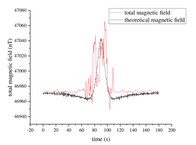
Fig. 18. Comparison between theoretical magnetic field and total magnetic field measured by experiment. |
The results revealed that the total magnetic field measured by the experiment had the magnetic anomaly waveform characteristics of submarine pipelines. Moreover, the magnetic anomaly detection function of the magnetic detection array is described in Section 2.2.3. Hence, this information infers that the suspected target may be the submarine pipeline without prior knowledge. Moreover, the suspected target is the submarine pipeline with prior knowledge.
Therefore, the offshore magnetic anomaly detection experiment of submarine pipelines verifies the function of the system to detect magnetic anomaly of submarine pipelines.
4. Conclusion
This study established a mathematical model of a two-part towed platform, including a spring-damping model of a secondary towed cable and a kinematic and dynamic model of a secondary towed vehicle. Considering the strong nonlinearity and time-varying characteristics of the platform, a self-adaptive fuzzy PID controller was designed for the constant altitude sailing of the two-part towed platform. Then, according to the magnetic anomaly detection theory of submarine pipelines, the magnetic anomaly model of submarine pipelines was established. In addition, the magnetic anomaly of submarine pipelines was calculated theoretically, and the magnetic detection array on the two-part towed platform was designed. Finally, the experimental verification of the magnetic detection system for submarine pipelines was conducted.
The experimental verification research shows that the constant altitude sailing experiment of the two-part towed platform verifies that the platform has good constant altitude sailing ability in both a hydrostatic environment and the actual marine environment. Meanwhile, the offshore magnetic anomaly detection experiment of submarine pipelines verifies the stable measurement function of the magnetic field and the function of the system to detect magnetic anomaly of submarine pipelines.
This research can provide theoretical support and experimental reference for the practical application of the magnetic detection system for submarine pipelines based on the two-part towed platform.
Declaration of Competing Interest
The authors declare that they have no known competing financial interests or personal relationships that could have appeared to influence the work reported in this paper.
Acknowledgement
The authors gratefully acknowledge the support of the Fund of State Key Laboratory of Ocean Engineering (GKZD010068; GKZD010074; GKZD010075).
