
1. Introduction
Deep-sea resources are extremely rich, and underwater vehicles are important types of equipment for exploring the deep sea. As the core component of a underwater vehicle, pressure hulls provide protection for the normal operation of the non-pressure-resistant equipment inside the underwater vehicle. Ceramic material has high strength, low density, and wear resistance, and can greatly improve the performance of underwater vehicle. However, the brittleness of ceramics is the inherent weakness of this material. Due to human operation of deep-sea application, the pressure hull based on ceramic material is very easy to appear some defects, which is very difficult to find. These defects will greatly reduce the pressure resistance of ceramics and result in the ceramic pressure hull unable to withstand deep-sea pressure. Then the hollow ceramic pressure hull is crushed, and a destructive phenomenon - implosion occurs in the deep sea.
Implosion is the opposite of explosion, which refers to the collapse of a pressure hull inward due to the high external pressure and the low internal pressure. The occurrence process of implosion is as follows: when the pressure hull works in the ultra-high pressure environment, the pressure hull cannot withstand the current environmental pressure due to some undetected initial defects. The hollow ceramic pressure hull yields or buckles under the external load. The pressure hull is crushed, and the seawater contacts with the air in the original hollow ceramic pressure hull and squeezes the air cavity. In this process, the hydrostatic pressure of the flow field is converted into the fluid kinetic energy. After the flow compresses the internal air cavity to the minimum, the internal air will rebound outward and transmit the shock wave to the flow field. The shock wave pressure produced by an underwater implosion is very large, and this pressure is far greater than the ambient pressure. Once the amplitude exceeds the strength limit of the surrounding structure, the surrounding structure will collapse. Therefore, the implosion of a pressure hull in deep sea may cause chain-reaction implosion of multiple pressure hulls. When the “Nereus” underwater vehicle shown in Fig. 1 dove to approximately 9990 m deep-sea, due to the implosion of a hollow ceramic pressure hull, a huge shock wave was generated, which immediately triggered a chain-reaction implosion, and finally, the whole vehicle fragmented [1].
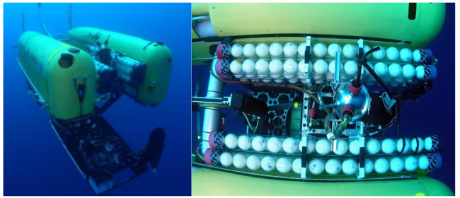
Fig. 1. Photographs of the “Nereus” vehicle (left) and its hollow ceramic pressure hulls (right) [2]. |
After the hollow ceramic pressure hull is crushed, the compression-rebound phenomenon of its internal air cavity is similar to bubble collapse. Rayleigh [3] studied the bubble collapse problem in 1917 and proposed the spherical bubble collapse theory to describe the growth and collapse of a single bubble in incompressible and inviscid flow. Based on this, considering the effects of liquid viscosity and surface tension, Plesset [4] derived the second-order nonlinear ordinary differential equation of the bubble radius varying with time, namely, the Rayleigh-Plesset equation. Keller and Miksis[5] considered the compressibility of liquid and proposed the more accurate Keller-Miksis equation to describe the bubble motion.
The bubble motion theory is mainly intended for the bubbles produced by underwater explosion. When the internal pressure is high, the bubbles expand, and when the internal pressure is lower than the hydrostatic pressure, the bubbles compress, thus repeatedly forming pulsations. The implosion of the ceramics pressure hull is because the hydrostatic pressure does work for the initial low-pressure air cavity after the ceramics pressure hull is crushed, and the kinetic energy of water increases continuously. In addition, the size of the ceramic pressure hull is much larger than that of the bubble. The research about bubble movement is focused on the change of the internal gas, but the implosion of the ceramic pressure hull is more focused on the propagation of the shock wave in the surrounding liquid.
Turner [6] used a hollow glass pressure hull to conduct an underwater implosion experiment in a 6.996 MPa cylindrical pressure vessel and obtained the shock wave pressure curve. Then the numerical simulation for the experiment was conducted using the software DYSMAS with an Eulerian fluid solver and a Lagrangian finite element solver. According to Turner's experiment, Morenko [7] used OpenFOAM software to simulate the implosion of a pressure hull based on the fluid volume method (VOF), and Morenko pointed out that increasing the gas pressure could effectively reduce the intensity of the implosion. It was also found that the larger the radius of the sphere was, the greater the pressure peak produced by the implosion was. Farhat et al. [8] conducted an implosion test on a small cylindrical metal shell and pointed out that the implosion pressure pulse was affected by the buckling mode and the failure position. Based on the principle of energy conservation, Zhipeng et al. [9] deduced a theoretical model for a spherical hull implosion in incompressible fluid and explored the relationship among the shock wave pressure, initial pressure, and sphere radius. Chamberlin et al. [10] proposed a measurement standard-based energy to divide the implosion energy of an underwater pressure hull into the initial energy (potential energy) in the system, the energy released into the fluid as a pressure pulse, the energy absorbed by the implosion structure, and the energy absorbed by the gas trapped in the pressure hull. According to the principle of a stress wave, Huang et al. [11] proposed an implosion test method for underwater hollow structures and tested the implosion of photomultiplier tubes at the pressure of 0.5 MPa. However, the previous research of underwater implosion was mainly focused on low pressure of underwater environment, and there is no public research about the underwater implosion of the hollow ceramic pressure hulls in 11,000 m depth.
Based on the compressible multiphase flow theory, the direct numerical simulation method and an adaptive rectangular grid are used to simulate the implosion of the hollow ceramic pressure hull. This method ignores the influence of structure and uses the same size spherical air cavity to replace the hollow ceramic pressure hull. In order to verify method proposed in this paper, the 6.996 MPa implosion experiment is simulated, and the peak value of pressure shock wave is slightly larger than the experimental results. This is because the structure of pressure hull is damaged into pieces at a low ambient pressure of 6.996 MPa, which can absorb a small part of implosion energy. So, the calculation results of the pure fluid numerical simulation method in this paper are slightly larger than the experimental results. Then, the underwater implosion in 11,000 m depth (115 MPa) is simulated and compared with the calculation results of fluid structure coupled method. The peak values of pressure shock wave obtained by the two methods are very close. This is because in 115 MPa ambient pressure, due to the brittleness of ceramic materials, the hollow ceramic pressure hull is damaged into powdery debris instantly, which almost not absorb the energy generated by implosion. Therefore, it is reasonable to ignore the influence of structure on implosion. The rationality and the accuracy of compressible multiphase flow method to simulate the implosion of hollow ceramic pressure hull in 11,000 m depth are verified. The shock wave calculation results of the two methods are close, but the compressible multiphase flow method is selected instead of the fluid structure coupled method. It is because the compressible multiphase flow method is a pure fluid simulation, and can capture the flow field information more precisely and accurately which can not be achieved by the fluid structure coupled method. Finally, the morphological evolution of air cavity and shock wave characteristics are analyzed, and the effects of different radii on the implosion shock wave characteristics of the pressure hull are simulated and analyzed. This study also describes the study of the implosion of two spheres. The different distances between the spheres are set to study the mutual influence of different placement distances on the implosion of the two spheres. In addition, the implosion of three spheres arranged linearly is studied.
2. Numerical method
In this section, the numerical simulation method of implosion of hollow ceramic pressure hull in ultra-high pressure environment is proposed. Firstly, according to the implosion characteristics of hollow ceramic pressure hull in ultra-high pressure environment, the calculation assumption and the model simplification based on compressible multiphase flow are proposed. Then the mathematical model of compressible multiphase flow and the equation of state of air and water are introduced. Finally, the grid and detailed setting of numerical simulation method are introduced.
The numerical simulation of this research uses the open source code ECOGEN [12] based on C++ that was developed to solve the compressible multiphase flow problem. The code integrates a variety of mathematical models, and its feasibility and accuracy have been verified for a variety of physical problems, such as bubble collapses, shock tubes, shock impact helium bubbles, water droplet atomization, and surface tension [13], [14], [15], [16].
2.1. The calculation assumptions and the model simplification
In order to prove the rationality of the calculation assumptions and the model simplification proposed in this paper, firstly, the material parameters of hollow ceramic pressure hull and the occurrence process of implosion are described. The characteristics of implosion are analyzed as the basis of supporting the assumption of numerical simulation.
The parameters of hollow ceramic pressure hull are shown in the Table 1, which is the hollow ceramic pressure hull once used on the "Nereus" underwater vehicle. Steve et al. [17] have conducted research on design, manufacturing, structural performance and quality control of the hollow ceramic pressure hull. The research shows that it is a seamless thin-walled hollow sphere made of Al2O3 ceramic material, with a diameter of 3.6 inches and a wall thickness of 0.058 inches (1.5 mm). The inside of the sphere is the atmospheric air.
Table 1. The parameters of hollow ceramic pressure hull. |
| Slurry composition | 99.9% Al2O3 | 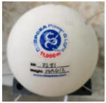 |
| Weight | 140 ± 1 g | |
| Average tdickness | 0.058 inches | |
| Outside diameter | 3.60 ± 0.05 inches | |
| Diameter variation on each sphere | ± 0.03 inches max |
The occurrence process of implosion is shown in Fig. 2. At the initial moment, the hollow ceramic pressure hull can't bear the ultra-high pressure in the deep sea due to some initial defects, and is instantly crushed into powder. Fig. 3 shows the powdered debris of the hollow ceramic pressure hull formed after implosion at 115 MPa. It is obviously that the hollow ceramic pressure hull could not absorb deformation energy like metal material pressure hull, so the influence of structure on the implosion flow field of the ceramic pressure hull can be neglected, which is validated in the Section 3.2.3. Because the pressure of the air cavity is far less than the ambient pressure, the seawater compresses the air cavity rapidly inward. The hydrostatic pressure is converted into the fluid kinetic energy, and a huge shock wave propagates outward after the air cavity is compressed to the minimum.
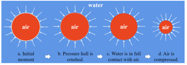
Fig. 2. The schematic diagram of implosion process. |
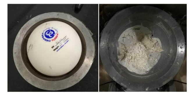
Fig. 3. Ceramic sphere and its powder after implosion. |
It can be seen that the underwater implosion of the hollow ceramic pressure hull under the ultra-high pressure environment has the following characteristics: at 115 MPa ultra-high pressure of 11,000 m depth, the ceramic pressure hull will be directly crushed into powder in case of implosion due to some undetected initial defects, without the phenomenon of large deformation and energy absorption similar to the metal pressure hull. Moreover, the ceramic pressure hull is completely damaged and forms powdered debris. The particle size is very small, and the fluid structure coupled phenomenon of pressure hull is not obvious. The implosion energy is mainly transmitted outward by the shock wave formed by the flow field.
Therefore, the destructive impact caused by implosion mainly comes from the fluid kinetic energy transformed by the pressure difference of the two phases gas-liquid after the hollow ceramic pressure hull is damaged. The damage of ceramic pressure hull has little effect on the implosion shock wave, which can be ignored in order to simplify the calculation. Based on these characteristics, the crushing process of hollow ceramic pressure hull in this paper is assumed as follows:
(1) The crushing time of hollow ceramic pressure hull accounts for a small proportion of the whole implosion time, and it is considered that the hollow ceramic pressure hull completes the crushing instantly.
(2) Ignoring the influence of implosion debris of the hollow ceramic pressure hull on the flow field, a spherical air cavity is used to replace the hollow ceramic ball and its internal air cavity.
Therefore, based on the above assumptions, the implosion of hollow ceramic pressure hull is simplified as: the numerical simulation based on compressible multiphase flow of the pressure shock wave propagating in water during collapsing of the spherical air cavity in ultra-high pressure water environment. Morenko [7] simplified the thin-walled glass ball containing air into a spherical air cavity. Based on the volume of fluid method (VOF), OpenFOAM was used to simulate the Turner's implosion experiment of glass sphere, which was in good agreement with the experimental results. Morenko also pointed out that it is important to know the hydrodynamic characteristics and detailed process data in the absence of the pressure hull. The numerical simulation can compensate for the shortcomings of the experimental technique by providing detailed information about the process. The comparison between absence and presence of the pressure hull is given to validate the above calculation assumption in the Section 3.2.3.
2.2. Kapila five-equation model for compressible multiphase flow
The numerical simulation of deep-sea implosion involves two phases of water and air, and water is considered to be a compressible fluid at ultra-high pressure with a depth of 11,000 m. Therefore, a compressible multiphase flow model is needed to simulate this problem. The Kapila five-equation model is widely used to simulate compressible multiphase flow [18], which is a simplification of the seven-equation model [19]. The model assumes that the velocity and pressure between the two phases are always continuous, which is based on the fact that in most problems of two-phase flow, the characteristic time required for the two phases to reach velocity equilibrium and pressure equilibrium is extremely short. The hyperbolic model of Kapila includes the evolution equation of the volume fraction, the continuity equation of the two phases, the momentum equation, and the energy equation of the mixture. It is written as Eq. (1)
$\left\{\begin{array}{ll} \frac{\partial \alpha_{1}}{\partial t}+\mathbf{u} \cdot \nabla \alpha_{1} & =K \nabla \cdot \mathbf{u} \\ \frac{\partial \alpha_{1} \rho_{1}}{\partial t}+\nabla \cdot\left(\alpha_{1} \rho_{1} \mathbf{u}\right) & =0 \\ \frac{\partial \rho_{2} \rho_{2}}{\partial t}+\nabla \cdot\left(\alpha_{2} \rho_{2} \mathbf{u}\right) & =0 \\ \frac{\partial \rho \mathbf{u}}{\partial t}+\nabla \cdot(\rho \mathbf{u} \otimes \mathbf{u}+p \mathbf{I}) & =0 \\ \frac{\partial \rho E}{\partial t}+\nabla \cdot((\rho E+p) \mathbf{u}) & =0 \end{array}\right. $
where the subscripts 1 and 2 are the two phases. αk is the volume fraction of phase k. ρk is the density of phase k. u and p are the velocity and pressure of the mixture. ρ=∑kαkρk, is the density of the mixture, and E = e + 0.5||u||2 is the total energy of the mixture, where e is the internal energy. The term K∇⋅u is the expansion and compression of each phase in the mixture regions, where K is given by Eq. (2)
$K=\frac{\rho_{2} c_{2}^{2}-\rho_{1} c_{1}^{2}}{\frac{\rho_{2} c_{2}^{2}}{\alpha_{2}}+\frac{\rho_{1} c_{1}^{2}}{\alpha_{1}}}$,
where ck is the speed of sound of phase k.
2.3. Equation of state
In this study, the ideal gas equation of state is employed, as shown in Eq. (3), where p is the pressure, V is the volume, n is the number of moles, R is the universal gas constant, and T is the temperature.
$P V=n R T$
In conventional numerical simulations, water is usually set as an incompressible fluid, that is, its density remains constant in the calculation. However, the implosion of the pressure hull of a underwater vehicle in 11,000 m depth is a strong impact and ultra-high pressure problem, and water is a compressible fluid in this environment. In this study, the equation of state of water uses the Stiffened-Gas equation of state [20], which can describe the state of liquid under high pressure well. This equation has been widely used in the fields of sonoluminescence, acoustic shock gravel, underwater nuclear explosion and so on. The Stiffened-Gas equation of state is shown in Eq. (4). Eq. (5) is the sound velocity calculation formula.
$P=(\gamma-1) \rho e-\gamma P_{\infty},$
$c^{2}=\frac{\gamma\left(P+P_{\infty}\right)}{\rho}$
where γ is the heat capacity ratio, e is the internal energy per unit mass, and P∞ is the pressure constant; When P∞=0, the Stiffened-Gas equation of state becomes the ideal gas equation of state. It can be seen that the ideal gas equation of state is a special form of the Stiffened-Gas equation of state.
2.4. Setting of the numerical simulation
The two-dimensional axisymmetric model is used to simulate the implosion of a single pressure sphere. As shown in Fig. 4, the center of the sphere is at the origin of the computational domain, and the side length is 10 times the radius of the sphere. The non-reflecting boundary conditions used in the calculation domain can effectively simulate the infinite sea pressure conditions in the environment of deep sea and eliminate the influence of the boundary shape on the simulation.
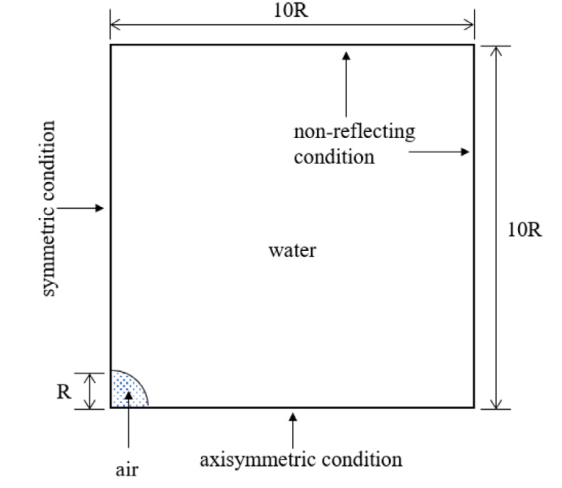
Fig. 4. Schematic of implosion of single spherical pressure hull. |
To effectively capture the changes in the shape of the sphere during the implosion process, as well as the propagation of expansion waves and compression waves, and to improve the accuracy of the simulation, three layers of adaptive mesh refinement (AMR) [21] are applied based on a uniform background of Cartesian grids, as shown in Fig. 5.
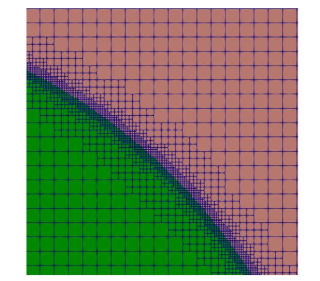
Fig. 5. Adaptive Cartesian grids. |
The initial conditions of the calculation are as follows: ideal gas is used to simulate the air inside the sphere, and the pressure is set to 0.1 MPa. The initial pressure of water is 115 MPa, and the initial velocity of the calculation domain is zero. The stiffened-gas parameters for the water are γw=4.4, and P∞=6 × 10⁸ Pa, and the ideal-gas parameter for the air inside the bubble is γb=1.4.
The implosion of two spheres is studied. The distances between the spheres are set to 4 cm, 6 cm, 8 cm, and 10 cm to study the mutual influence of different placement distances on the implosion of the two spheres. The implosion of three spheres arranged linearly is also studied.
3. Verification of the method
3.1. Verification of the 6.996 MPa calculation
3.1.1. Grid convergence
To verify the convergence of the grids, the following three sizes of grids are used in the simulation of the implosion of a single sphere under pressure at 6.996 MPa: 200 × 200, 400 × 400, and 800 × 800. Three layers of AMR are applied for these three background grids. Table 2 is the pressure peak at the monitoring point and the air cavity collapse time at 6.996 MPa in different grids.
Table 2. The pressure peak at the monitoring point and the air cavity collapse time at 6.996 MPa. |
| Background grids | Pressure peak at monitoring point (MPa) | Air cavity collapse time (ms) |
|---|---|---|
| 200 × 200 | 40.6 | 0.421 |
| 400 × 400 | 41.0 | 0.418 |
| 800 × 800 | 41.1 | 0.417 |
According to the Computational Fluid Dynamics (CFD) uncertainty analysis method proposed by ITTC [22], the convergence of the grid can be verified, three groups of 200 × 200, 400 × 400, and 800 × 800 grids are selected, and the verification method is as follows:
The convergence ratio R is defined as R = ε32/ε21.
Here, ε2 =S2−S1, ε32=S3−S2. S1, S2, and S3 are the simulation results for a coarse grid, medium grid, and fine grid, respectively. The relationships between the convergence state and the convergence ratio R are
(1) Monotone convergence: 0 < R < 1;
(2) Oscillatory convergence: R < 0;
(3) Divergence: R > 1.
The convergence ratios R of the pressure peak and the collapse time calculated with this method are 0.25 and 0.33, respectively, and they are both less than 1, which conforms to the convergence criterion. Therefore, considering the accuracy of the simulation and the computational cost, a400 ×× 400 grid is used for further calculation.
3.1.2. Verification of pressure shock wave results
In order to verify the feasibility and the accuracy of the numerical simulation method, Turner's implosion experiment of glass sphere is simulated based on this method. Turner used a thin-walled glass sphere with a radius of 3.81 cm and a thickness of 0.762 mm, filled with the water and pressurized to 6.996 MPa in a pressure cylinder with a diameter of 1.52 m and a length of 3.66 m. As shown in Fig. 6, three pressure sensors are set at equal intervals at a distance of 10.16 cm from the spherical center. In the experiment, in order to detonate the glass sphere, the hydraulic device was started, and the trigger was driven to knock the glass sphere to break it, so as to produce implosion.

Fig. 6. The schematic diagram of Turner's experiment. |
In Fig. 7, the pressure at the detection point 10.16 cm from the center of the sphere in the Turner's experiment and the compressible multiphase flow method is presented. Table 3 shows the pressure peak of the shock wave at 10.16 cm from the center of the sphere. The reason why the result of the compressible multiphase flow method is larger than the experimental result is that the simulation does not consider the glass shell of the sphere, which absorbs part of the energy when it collapses.
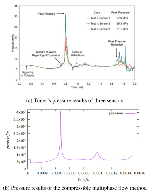
Fig. 7. Pressure at 10.16 cm from the center of the sphere under 6.996 MPa. |
Table 3. The pressure peak of the shock wave at 10.16 cm from the center of the sphere under 6.996 MPa. |
| Source | The pressure peak of the shock wave (MPa) |
|---|---|
| Tuner's experiment | 25.3, 27.0, 31.1 |
| Tuner's simulation of DYSMAS | 38.4 |
| The simulation of present research | 41.0 |
3.1.3. Verification of radius evolution of the air cavity at 6.996 MPa
In the bubble collapse theory, the Keller-Miksis (K-M) equation considers the compressibility of water based on the Rayleigh Plesset equation [5], which has been widely recognized and which can be used to verify the radius evolution after sphere implosion. In this study, the K-M equation is used in the following form as Eq. (6):
$\frac{3}{2}\left(1-\frac{\dot{R}}{3 c_{L}}\right) \dot{R}^{2}+\left(1-\frac{\dot{R}}{c_{L}}\right) R \ddot{R}=\frac{1}{\rho_{L}}\left(1+\frac{\dot{R}}{c_{L}}+\frac{R}{c_{L}} \frac{\mathrm{d}}{\mathrm{dt}}\right)\left(P_{g 0} \frac{R_{0}^{3 \gamma}}{R^{3 \gamma}}-P_{0}\right)$
where R represents the radius of the air cavity, cL represents the sound velocity in water, ρL represents the density of water, Pg0 represents the internal pressure of the air cavity at the initial time, P0 represents the ambient pressure of water, and γ is the heat capacity ratio. γ= 1.4 for air.
Using the Runge-Kutta method to solve the above equation, the variation curve of the sphere radius with time can be obtained. The accuracy of the numerical simulation can be verified by comparing the numerical simulation with the radius change curve in the numerical simulation.
Fig. 8 shows the evolution of the sphere radius given by the simulation of the implosion of a single sphere and the change of the radius R given by the semi-analytic solution of the Keller-Miksis equation considering the compressibility effect. These two curves fit well. In particular, before the second compression, the two curves are almost identical. It can be seen from the figure that there is an obvious compression-rebound phenomenon in the implosion at the pressure of 6.996 MPa. The initial radius of the sphere is 3.81 cm, and compression to 0.42 cm occurs at 0.418 milliseconds, which is about 11% of the initial radius, and then the radius rebounds to 2.24 cm at 0.67 milliseconds, which is about 59% of the initial radius. In the initial stage of implosion, the low-pressure air cavity is compressed by the high pressure of the liquid phase. The air cavity is an ideal gas, and the pressure increases due to the decrease of the air cavity's volume. When the pressures inside and outside of the air cavity interface are equal, the air cavity continues to compress inward due to inertia. After the sphere air cavity is compressed to the minimum volume for the first time, the sphere air cavity enters the rebound stage because the internal pressure is much greater than the ambient pressure. After rebounding to a certain stage, the pressures inside and outside of the air cavity reach equilibrium again, and the air cavity continues to rebound outward due to inertia. When the interface velocity of the air cavity reaches zero, the air cavity begins to rebound again due to the existence of an internal and external pressure difference. After multiple compression-rebound processes, the internal and external pressures of the air cavity finally reach equilibrium, and its interface velocity is zero. Finally, the volume of the air cavity does not change.
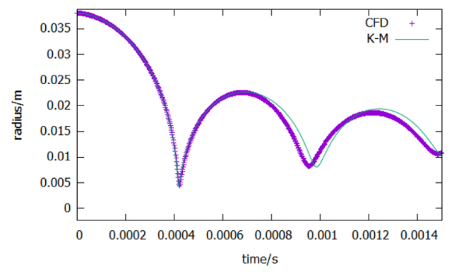
Fig. 8. Radius evolution at 6.996 MPa. |
3.2. Verification of the 115 MPa calculation
3.2.1. Grid convergence
The implosion of the hollow ceramic pressure hull at 115 MPa is numerically simulated. To verify the convergence of the grid, the following five sizes of grids are used in the simulation of the implosion of a single sphere under pressure at 115 MPa: 50 × 50, 100 × 100, 200 × 200, 400 × 400, and 800 × 800. The pressure of the monitoring point 10 cm from the center of the sphere of different grids is shown in Fig. 9. It can be seen from the curves of the pressure peak of the shock wave with different grids that the pressure peak and its corresponding time for a 400 × 400 grid and an 800 × 800 grid are very close. Table 4 is the pressure peak at the monitoring point and the air cavity collapse time at 115 MPa in different grids.
Fig. 9. Pressure peak at the monitoring point and the air cavity collapse time at 115 MPa in different grids. |
Table 4. The pressure peak at the monitoring point and the air cavity collapse time at 115 MPa. |
| Background grids | Pressure peak at monitoring point (MPa) | Air cavity collapse time (ms) |
|---|---|---|
| 50 × 50 | 403 | 0.158 |
| 100 × 100 | 416 | 0.143 |
| 200 × 200 | 427 | 0.131 |
| 400 × 400 | 434 | 0.123 |
| 800 × 800 | 438 | 0.122 |
| R | 0.571 | 0.125 |
The convergence ratio R mentioned in Section 3.1.1 is also used to judge the grid convergence. The convergence ratios R of the pressure peak and the collapse time calculated with this method are 0.571 and 0.125, respectively, and they are both less than 1, which conforms to the convergence criterion. Therefore, a 400 × 400 grid is used for further calculation.
3.2.2. Verification of radius evolution of the air cavity at 115 MPa
With this ambient pressure, the implosion of a sphere with a radius of 5 cm is analyzed. Fig. 10 shows how the radius changes over time. The radius curve output by the result of the numerical simulation is in agreement with the Keller-Miksis equation in the compression stage. The air cavity compresses to the smallest volume at 0.123 milliseconds and then rebounds. The radius curve in the rebound stage is relatively flat, and the subsequent fluctuations are not as obvious as the curve of the Keller-Miksis equation. The main reason is that the derivation of the Keller-Miksis equation is based on the small interface Mach number, while the Mach number in the compression stage of this simulation reaches 1.1 or more.
Fig. 10. Radius evolution at 115 MPa. |
Comparing the calculation results for 115 MPa and 6.996 MPa, it can be found that with the premise that the initial pressure of the internal gas is 0.1 MPa, the rebound of a 115 MPa single sphere after compression to the smallest volume is obviously weaker. The main reason for this is that although the greater external pressure produces a greater pressure peak produced with the implosion, the energy required to promote the outward diffusion of water at an ambient pressure of 115 MPa is much greater than that of achieving the same effect in an environment of 6.996 MPa.
3.2.3. Verification with fluid structure coupled method
In this section, a multiphase fluid structure interaction (FSI) model of the underwater implosion was proposed. This model was developed using ABAQUS/explicit CEL (Coupled Eulerian Lagrangian) method. The CEL method includes two explicit solvers: Euler fluid solver (Solving the Navier-Stokes equation) and Lagrange finite element solver (solving the material stress, strain, deformation, displacement, velocity and acceleration). An Eulerian mesh with hexahedral Euler element (EC3D8R) is created for the fluid phase, which includes the sea water phase and the air phase. The media is tracked based on the volume-of-fluid method (VOF). A Lagrangian mesh is created for the hollow spherical pressure hull with 3D hexahedral C3D8R elements, and the computational domain mesh is shown in Fig. 11. The hollow ceramic sphere is made of 99.9% Al2O3 ceramics, and the material properties are described in Section 2.1. The brittle fracture criterion is adopted for the ceramics, that is, the ceramic unit begins to fail at the maximum principal stress of 310 MPa, and then the ceramic unit is removed from the solid structure.

Fig. 11. Calculation domain and mesh diagram of the CEL method. |
The hollow ceramic pressure hull selected in the study will not be damaged under the hydrostatic pressure. In order to detonate the hollow ceramic pressure hull, a pair of extrusion balance forces acting on both sides of the ball along the Z direction are applied at the initial time, as shown in Fig. 12. Outside the hollow ceramic pressure hull, a monitoring point is set at twice radius from the spherical center to record the peak value of pressure shock wave at this position, and compared with the numerical simulation results based on compressible multiphase flow. It can be seen from Fig. 13 that the peak value of pressure shock wave in CEL method is 3% smaller than that in compressible multiphase flow method. The reason is that the crushed ceramic particles absorb a small part of energy after implosion, and the impact of this part is very small. In order to simplify the calculation, it is considered that the weak influence of the structure can be ignored. Therefore, the compressible multiphase flow method proposed in this paper is feasible and accurate to calculate the implosion of hollow ceramic pressure hull at 11,000 m depth ultra-high pressure.
Fig. 12. Extrusion equilibrium force acting on both sides of the sphere along the Z direction. |
Fig. 13. Comparison of pressure between the compressible multiphase flow method and CEL method. |
4. Results
4.1. The results of implosion of single sphere at 115 MPa
4.1.1. Analysis of pressure shock wave results
Fig. 14 shows the pressure curves of different monitoring points outside the sphere during the implosion of a single spherical ceramic pressure hull at the pressure of 115 MPa. In the compression stage, due to the external seawater flowing into the air cavity, sparse waves are transmitted from the outside of the air cavity, which results in a pressure-drop on the outside of the sphere during the initial stage of implosion. As shown in Fig. 14, the magnitude of the pressure drop decreases from the surface of the sphere outward. The pressure drops 83.5% from 115 MPa to 19 MPa at the monitoring point 6 cm from the spherical center.
Fig. 14. Pressures at different points at 115 MPA. |
The process of the pressure drops at the monitoring point outside the sphere lasts for a very short time, and the pressure gradually rises after reaching the minimum value. In 0.123 milliseconds (from Fig. 10), the volume of the air cavity is compressed to the minimum, its pressure increases sharply, and the compression wave is rapidly transmitted outward, causing the pressure of the detection point outside the sphere to increase rapidly. Since the compression wave needs to do work on the water during its outward transmission, the farther the monitoring point is from the spherical center, the smaller the pressure peak that can be reached is. The pressure peak at the monitoring point 6 cm away from the spherical center reaches 774 MPa, which is about 6.7 times the ambient pressure. At the monitoring point 12 cm away from the spherical center, the pressure peak reaches 364 MPa, slightly greater than three times the initial value. After analyzing the numerical results, an approximate formula for the relationship between the distance to the spherical center and the peak pressure of the shock wave is proposed.
$P_{\text {peak }}=115+7100 x^{-1.343}$
where Ppeak is the pressure peak of shock wave gotten by the fitting curve, and x is the distance to the center of sphere.
Fig. 15 shows the results of the numerical simulation and the approximate formula, and they are in good agreement. According to the fitting curve in the figure, the pressure peak of shock wave attenuates rapidly. At a distance of 30 cm from the spherical center, the pressure peak of shock wave is already very close to the ambient pressure. Fig. 16 shows the pressure cloud of the shock wave at 115 MPa.

Fig. 15. Relationship between peak pressure and position. |
Fig. 16. Pressure cloud of shock wave at 115 MPa. |
The propagation speed of the shock wave is calculated with the time when the shock wave arrives at each monitoring point as shown in Fig. 17. At the pressure of 115 MPa, the shock wave has a very large propagation speed, which is close to the sound speed in this environment, and as the propagation distance increases, the shock wave speed decreases slowly.

Fig. 17. Speed of shock wave with distance. |
4.1.2. Analysis of implosion pressure with different radii
To study the rules of the implosion of the spheres with different radii for a pressure of 115 MPa, implosion simulations are performed for spheres with radii of 1 cm, 3 cm, 5 cm, 7 cm, and 9 cm. Fig. 18 shows the pressure peak of the shock wave with different spheres radii at the monitoring point 10 cm away from the spherical center. The fitting formula is given based on the simulated value as Eq. (8):
$P_{\text {peak }-R}=86.39 R+34.93$
where Ppeak-R is the pressure peak with radius of shock wave gotten by the fitting curve, and R is the radius of sphere.
Fig. 18. Peak pressure 10 cm from the spherical center for different radii. |
It can be seen that the peak pressure at the monitoring point is close to a proportional relationship with the radius of the sphere. At an ambient pressure of 115 MPa, for every 1 cm increase in the radius of the sphere, after the implosion, the pressure peak at the monitoring point 10 cm from the spherical center increases by about 86.4 MPa.
4.2. The results of the implosion of two spheres at 115 MPa
4.2.1. Setting of the implosion of two spheres at 115 MPa
In the actual deep-sea condition, the large pressure generated by the implosion of a single ceramic pressure hull is transmitted outward in a very short time, and the shock wave that is several times the ambient pressure destroys the surrounding ceramic pressure hulls and causes them to occur implosion, and so on until all ceramic pressure hulls are damaged. This type of extremely destructive chain reaction is called a chain-reaction implosion.
Studying the implosion of two spheres and multiple spheres is of great significance for exploring the mechanism of chain-reaction implosion. The real process of the chain-reaction implosion is that each ceramic pressure hull occurs the implosion in turn. To simulate the real sequential implosion, the material properties of the structure and the simulation of the fluid-structure interaction need to be considered. Since this study only considers fluid simulation, the strategy used here is that two spheres or multiple spheres implode at the same time, which is a simplification and also a limit state of sequential implosion. The destructive force produced in this way is greater than that of sequential implosion.
Fig. 19 is the schematic diagram of the implosion of two spheres. The distance d between the spheres is set to 4 cm, 6 cm, 8 cm, and 10 cm to compare the influence of different spacing on the implosion of the two spheres. The influences of the effects of pressure superposition are studied. Since the centers of the two spheres can be connected to form a symmetry axis, a two-dimensional axisymmetric model can still be used.

Fig. 19. Schematic of implosion of two spheres. |
4.2.2. Analysis of pressure shock wave results
Fig. 20 shows the pressure cloud at different moments in the implosion of two spheres that are 6 cm apart. In the initial stage of the implosion, the water surges into the air cavity. The air cavity propagates the expansion wave outward, and the area where the expansion wave passes produces a pressure drop, as shown in the pressure cloud chart at 0.016 ms. At 0.03 ms, the expansion waves generated by the two spheres converge at the center of the two spheres, forming a superposition, and the pressure drop in the superimposed area is greater. As shown for 0.06 ms and 0.08 ms, the area covered by the expansion wave continues to expand, and the superimposition range of the expansion wave gradually covers the area where the two spheres are located.
Fig. 20. Pressure cloud of implosion when two spheres are 6 cm apart (Pressure/Pa). |
As the volume of the spherical air cavity continues to compress, its internal pressure continues to increase. The air cavity begins to rebound after its volume is compressed to a minimum, and the large internal pressure spreads outward in the form of shock waves. The pressure of the shock wave on the inner side between the two spheres is much higher than that on the outer side. The two shock waves converge at the center of the two spheres, forming a high-pressure zone. As the shock wave spreads outward, the superimposed high-pressure zone keeps moving away from the central area of the spheres and is always maintained in the vertical direction of the centers of the two spheres.
4.2.3. Analysis of implosion pressure with different spacing
Two groups of monitoring points are set in the calculation domain. The first group of monitoring points is in position 1 as shown in Fig. 21, which is located on the outside of the two spheres and on the axisymmetric boundary. The second group of monitoring points is in position 2 as shown in Fig. 21, which is located between the two spheres and on the perpendicular bisector of the connecting line between the centers of two spheres.

Fig. 21. The position of the monitoring points. |
Firstly, the pressure peak of shock wave at the monitoring points at position 1 is analyzed. From Fig. 22, there are two obvious peaks in the pressure at this position. The first peak is mainly caused by the compression wave transmitted by the implosion of the sphere on the left. The monitoring point 5 cm away from the surface of the sphere is taken as an example. Table 5 shows the comparison the pressure peak of the first shock wave with the pressure peak of the shock wave of a single sphere implosion. It can be seen that this peak value is less than the value of the implosion of a single sphere due to the interaction between two spheres. The smaller the distance between the two spheres is, the more obvious the interaction is, and the smaller the first peak pressure is. The second peak pressure at this position is the compression wave transmitted by the right sphere which propagates from between the two spheres. The compression wave between the two spheres would be analyzed at the monitoring points at position 2.
Fig. 22. Pressure curve of the left monitoring points with different sphere spacing. |
Table 5. The first peak pressure at the monitoring point 5 cm from the surface of the left sphere. |
| The spacing between the two spheres/cm | The first peak pressure/MPa |
|---|---|
| 4 | 194 |
| 6 | 214 |
| 8 | 246 |
| 10 | 299 |
| The pressure peak of the implosion of a single sphere | 434 |
Fig. 23 shows the pressure of the monitoring points in position 2. The monitoring points at this position is used to analyze the pressure shock wave characteristics between the two spheres. The pressure shock wave here is the superposition of two implosion shock waves, and the pressure peak of the superimposed shock wave is huge. The research of this superimposed shock wave is of great practical engineering significance. The smaller the distance between the two spheres is, the greater the pressure is. Taking the monitoring point 5 cm from the axisymmetric boundary as an example, when the distances between the spheres are 4 cm, 6 cm, 8 cm, and 10 cm, the pressure peaks reach 1258 MPa, 1049 MPa, 828 MPa, and 721 MPa, respectively.
Fig. 23. The pressure of the monitoring points in the vertical direction of the center of the two spheres with different sphere spacing. |
Next, the superimposed shock wave value of the implosion of two spheres and twice the shock wave value of the implosion of a single sphere are compared. First, the distances between the monitoring points and the spherical center are calculated in Eq. (9), as shown in Fig. 24.
$x=\sqrt{\left(R+\frac{d}{2}\right)^{2}+h^{2}}$

Fig. 24. Location of monitoring points. |
By substituting the value of x into Eq. (7), and the pressure shock wave P1 of the implosion of a single sphere at the position x away from the spherical center is obtained. Then 2P1 is compared with the pressure shock wave P2 of the implosion of two spheres at the monitoring points. The superposition rate is defined as Eq. (10)
$\delta=P_{2} / 2 P_{1}$
If δ>1, it shows that the superposition of the implosion of two spheres can enhance the shock wave, and a stronger shock wave will be formed when two shock waves meet. This phenomenon is called the superposition effect of shock waves as shown in Fig. 25.ε is the ratio of the distance between the monitoring point and the spherical center to the spherical radius (ε= x/R). Fig. 26 shows the curves of δ and ε for different spacing between two spheres.
Fig. 25. Superposition effect. |
Fig. 26. The curves of δ and ε for different spacing between two spheres. |
As can be seen from the Fig. 26, when the distances between the two spheres are 4 cm, and 6 cm, some parts of ε appear δ>1, that is, the superposition effect enhances the strength of the shock wave. As the shock wave propagates outward, δ gradually decreases; that is, the superposition effect of the shock wave gradually weakens. And the superposition effect decreases with the increase of the spacing between two spheres. When the spacing is greater than 1.6R, there is already no superposition effect. And it can be analyzed the reason why δ<1 from the pressure cloud of implosion of two spheres. The implosion shock wave of two spheres is no longer the circle of uniform pressure distribution during a single sphere implosion, but the high-pressure area converges between the two spheres as shown in Fig. 27. The pressure outside the two spheres decreases obviously, which is the reason why the pressure shock wave at the monitoring points of position 1 is less than a single sphere implosion. When the distance between the two spheres is too large, the shock wave is superimposed at the position lower than the single sphere implosion, so δ<1. Therefore, it can be seen that the study of the implosion of two spheres is very meaningful. More attention should be paid to the superposition effect when the distance between the two spheres is small, which makes the destructive power of the shock wave greater. Therefore, it can be concluded that when analyzing multi spheres implosion, it can't be simply considered as a multiple relationship.
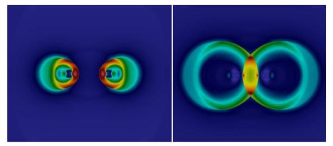
Fig. 27. The high pressure area of the shock wave converges between the two spheres. |
4.3. The results of implosion of three spheres under 115 MPa
At last, the implosion of the three spheres on a straight line is simulated, but only the preliminary phenomenon analysis of the pressure field is carried out. Fig. 28 displays the schematic diagram of the implosion of the three spheres. The distance between the spheres is set to 4 cm.
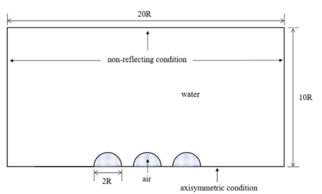
Fig. 28. Schematic of implosion of three spheres. |
Fig. 29 shows the pressure cloud of the implosion of three spheres at different times when the distance between the spheres is 4 cm. The variation law of the pressure field is similar to that of the implosion of two spheres. In the initial stage of implosion, seawater flows into the air cavity of the sphere, and the sphere transmits an expansion wave outward, resulting in a pressure drop in the area it passes through. After the expansion waves generated by the three spheres meet, these expansion waves are superimposed into a low-pressure area with less pressure.
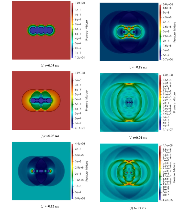
Fig. 29. Pressure cloud of implosion of three spheres at different times (Pressure/Pa). |
After the volume of the air cavity is compressed to the minimum, the huge pressure generated inside the air cavity is transmitted to the water in the form of a shock wave. The shock waves of the three spheres meet in pairs, forming a high-pressure area with greater pressure at the superposition of the shock waves. As can be seen from Fig. 29(d), the radius of the circular high-pressure area of the implosion shock wave of the middle sphere is smaller than that of the left and right spheres. The suppression effect of the left and right spheres on the implosion of the middle sphere makes the implosion shock wave of the middle sphere diffuse outward later than the implosion shock wave of the left and right sides. Therefore, the superposition position of the shock wave is not on the central axis of the two adjacent spheres, but rather gradually becomes close to the central axis of the three spheres. With the outward propagation of the shock wave, the superimposed high-pressure areas of the three shock waves are combined. This suppression effect mentioned earlier still needs more studies to verify, and no definite conclusion can be drawn here. This section is the preliminary exploration of implosion of the three spheres, and the law of chain-reaction implosion will be further studied in the future.
5. Conclusions
Based on the compressible multiphase flow theory and adaptive mesh refinement technique, the numerical simulation method of the underwater implosion of spherical hollow ceramic pressure hulls is proposed. In order to verify the method, the results of the numerical simulation are compared with the classical implosion experiment and the fluid structure coupled method. Then the radius evolution of the air cavity and the characteristics of pressure shock wave are studied. Finally, the implosion of two and three spherical hollow ceramic pressure hulls arranged linearly at a pressure of 115 MPa are simulated and analyzed.
The main conclusions of the above research content are as follows:
(1) The numerical simulation method based on compressible multiphase flow for the implosion of the hollow ceramic pressure hull at 11,000 m depth is accurate and the feasible.
(2) In the implosion of single sphere, the magnitude of the pressure shock wave due to the implosion is several times greater than that of the ambient pressure and attenuates rapidly with outward transmission. The transmission velocity of the shock wave is close to the sound velocity in water.
(3) In the implosion of two spheres, the implosion shock wave is no longer the circle of uniform pressure distribution, but the shock wave pressure between the two spheres increases, and the shock wave pressure outside the two spheres decreases. In the area between the two spheres, due to the existence of the superposition effect of shock wave, when the distance between two spheres is less than 1.3R, the stronger shock waves appear after the two shock waves meet.
(4) In the implosion of three spheres, the shock waves generated by different spheres converge with each other and finally form a high-pressure zone in the vertical direction of the sphere center connecting line. The influence of the left and right spheres on the implosion of the middle sphere makes the implosion shock wave of the middle sphere diffuse outward later than the implosion shock waves of the left and right sides.
Declaration of Competing Interest
The authors declared no potential conflicts of interest with respect to the research, authorship,and/or publication of this article.
Acknowledgement
The authors would like to deeply appreciate the support from the National Natural Sciences Foundation of China (51779139, U2067220), the National Key Research and Development Program of China (Grant No. 2016YFC0300700), Shanghai Talent Development Funding (2018029) and the Young Talent Project of China National Nuclear Corporation.
