
1. Introduction
Internal waves, commonly referred to as gravitational waves, are phenomena that arise within a geological fluid (such as the atmosphere, oceans, or lakes) and also on the surface of a part of it. For the phenomenon to occur, the stream must be stratified; each stratum should have the same viscosity and temperatures, which may only vary with elevation.The waves are transmitted continuously like vibrational modes when the concentration fluctuates over a moderate vertical position [1]. Internal waves in the atmosphere arise whenever a homogenous flow of wind passes above a main impediment, such as a mountainous region. Horizontal stripes of uniform wind are interrupted when the wind meets an obstruction, forming a wave formation. They can generate wave storms, which are generated when sustained wind passes over an obstruction like a mountain [2], [3]. Numerous researchers, including Bear [4], have addressed the Boussinesq equation as a mathematical model for shallow water waves in streams and oceans, laying the foundations for the idea of internal wave phenomena. Since then, the BSe type model have gained significance, with applications ranging from including internal gravity waves in lakes with various cross-sections, ion-acoustic waves in plasma, and inter-facial waves in a two-layer liquid with varying depths being identified [5].
The topic in this research work is of current interest and the results are essential in understanding various nonlinear wave phenomena. The N-soliton solutions of classical Boussinesq model equationare precisely expressed in Wronskian form [6]. Soliton solutions are essentially the solutions formulated from convergent series solutions that arise from many shallow water equations, particularly the Boussinesq equation, using either the Adomian decomposition method or the homotopy perturbation method. Some interesting very recent studies have been conducted by systematically studying the N-soliton solutions to nonlinear dispersive wave equations via the Hirota bilinear method for both (1+1)-dimensional equations [7] and (2+1)-dimensional equations [8] including some other novel essential classes of equations in (2+1)-dimensions [9], [10], [11].
Numerous researchers have analyzed fractional evolution equations in the last decade because of their enormous usefulness in multiple domains of development in science and engineering (see [14], [15], [16], [17], [18], [19], [20], [21], [22], [69] for more related studies about fractional differential equations). Eventually, these fractional evolution equations can describe a wide range of essential effects in quantum mechanics, hydrodynamics, chaos, fibres, bifurcation, acoustics, thermodynamics, aquifers, biology, diseases and material science, among other disciplines [10], [23], [24], [25], [26], [27], [28], [29], [30]. Furthermore, approximate findings of fractional evaluation equations are of considerable worth. Various initiatives can also be conducted to evaluate the dynamic behaviour of fractional systems. By employing linearization or series solutions, these analytical approaches are susceptible to achieving an estimated result. In this flow, several new definitions and fractional operators are introduced by numerous analysts, such as Caputo, Hadamard, Hilfer, Riez, Caputo-Fabrizio, and Atangana-Baleanu, that can portray physical phenomena accurately with memory depending on power law, exponential, and Mittag-Leffer as a kernel, see [31] and the references cited therein. In addition, the authors [31] expounded a new derivative known to be the Atangana-Baleanu (AB) fractional derivative, which has the kernel of a Mittag-Leffler type function. Kumar et al. [32] developed the approximate-analytical solution of the regularized long-wave model using the AB-fractional operator. Singh et al. [33] sought to characterize the kinetics of the AB-fractional operator using a Mittag-Leffler type function. In terms of representing physical challenges, the Mittag-Leffler function is significantly more effective than the power and exponential functions. As a result, the fractional derivative of the AB operator is well designed for resolving inhomogeneities in a wide range of substances, configurations, and interfaces. In the scientific research era, the invention of an integral transform can be attributed directly to P. S. Laplace’s (1749-1827) effort on probabilistic dynamics in the 1780s, as well as to J. B. Fourier’s (1768-1830) dissertation ”La Théorie Analytique de La chaleur” described in [34]. Following this propensity, Jafari [35] contemplated the generalized integral transform (GIT) is a significant transformation in its entirety. A variant of the GIT is the, Laplace, ρ-laplace, Elzaki, Aboodh, Natural, Swai, Sumudu, Kamal, Mohand, Pourreza, G-transform and Shehu transform, see [36], [37], [38], [39], [40], [41], [42], [43], [44], [45], [46], [47], [48].
Nonlinear equations are used to model the majority of scientific and engineering disciplines. Several engineers are fascinated by the necessity of discovering adequate solutions to this sort of equation employing mathematical or theoretical approaches. The bulk of scientific and technical disciplines rely on nonlinear equations to model their data. The necessity of using mathematical or theoretical methodologies to find suitable solutions to this type of equation fascinates many engineers involving multibody systems with springs [49], the study of vibration of the unsymmetrical laminated composite beam [50], conservative vibratory systems [51], beams resting on elastic foundations [52] and several other domains. Most classic perturbation approaches struggle to solve those equations due to their intricacy. Many innovative strategies are suggested to cope with this deficit in order to overcome this problem. Differential transform method (DTM) [53], homotopy analysis transform method (HATM) [54], variational iteration method (VIM) [55], Tanh method (TM) [56], He’s energy balance method (HEBM) [57], wavelet-collocation-based methods (WCM) [58], Backlund transformation methodologies (BTM) [59], inverse Laplace homotopy technique (ILHT) [60], reproducing kernel Hilbert space method (RKHSM) [61] are just a few examples.
Finding an effective fractional PDE in the framework of numerical techniques is a challenging task. It necessitates a comprehension of the underlying physical processes. On the other hand, realistic physical processes are always tempered with vagueness. This is evident when interacting with ”living” resources like soil, water, and microbial communities. Wave propagation in nonlinear and dissipation mediums is characterized by the BSe in hydrodynamics [62]. While there are some notable previous works related to ocean engineering and science that have been recently published such as the investigations of the generalized Schrödinger-Boussinesq equations for the interaction between complex short wave and real long wave envelope [63], (2+1) dimensional Bogoyavlensky-Konopelchenko equation with variable-coefficient in wave propagation [12], complex soliton solutions of the perturbed nonlinear Schrödinger equation in nonlinear optical fibers [13], the fifth-order KdV equation’s special case [64], the Mikhailov-Novikov-Wang equation [65], the generalized HirotaSatsumaIto and (3+1)-dimensional JimboMiwa equations [66] (see also [67]), and the generalized fuzzy transform [68], our work is original and unique with novel results because the proposed fuzzy fractional-order Boussinesq model in this work is new and has never been investigated in detail before in any other research works in ocean engineering which can provide new insights to understanding various oceanographic phenomena and many related future works can be based on the results in this research.
To achieve numerical solutions of fourth-order time-fractional BSe, we will employ the fuzzy generalised integral transform coupled with the ADM in this investigation. Bear [4] introduced the classical BSe in 1978, as follows:
$\frac{\partial}{\partial \mathbf{x}}\left(K_{\mathbf{x}} \Theta \frac{\partial \Theta}{\partial \mathbf{x}}\right)+\frac{\partial}{\partial \omega}\left(K_{\omega} \Theta \frac{\partial \Theta}{\partial \omega}\right)+W=U \frac{\partial \Theta}{\partial z}$
where Kx represents the saturated hydraulic conductivity in the x way $(S / \mathscr{T}) ; K_{\omega}$ denotes the saturated hydraulic conductivity in the ω direction $(S / \mathscr{T})$; Θ indicates the hydraulic head (S); U is the precise yield (dimensionless) and P named the recharge/discharge rate $(S / \mathscr{T})$.
Three hypotheses are taken into account when computing the fractional BSe:
i. Suppose that the Dupuit-Forchhimer claims are true, as well as Darcy’s law.
ii. In the control volume, the fluid (water) is non-compressible.
iii. The flux fluctuations in the control volume are governed by a power-law function.
The (1.1) equation was developed as part of research on wave propagation in shallow water. It was then developed to overcome water purification problems in porous subsurface strata. Furthermore, (1.1) is frequently deployed in coastal and ocean construction to solve water filtration problems in porous underground strata. BSe can also function as a methodology for a variety of models that interact with drained groundwater circulation and subsurface drainage. The fractional BSe are well adapted to investigating water transport over porous heterogeneous media. The authors [70] contemplated power law variations of flux in control volume and fractional Taylor sums to determine the fractional BSe. Periodic, soliton, and explosive waves solutions of BSe [71] were investigated using fractional variational methods. For the fractional BSe, Zhuang et al. [72] introduced two new computational approaches: finite volume and finite element approaches leveraging nodal dependent functions. Abassy et al. [73] developed a fractional BSe by applying modified VIM. Wu and Hsieh [74] improved linearized BSe solutions for a gradient aquifer with dynamically fluctuating rainfall.
On the other hand, conventional mathematics is incapable of dealing with this circumstance. As a result, alternative theories are required in order to address this problem. There are several frameworks for explaining this scenario, the most prominent of which is the fuzzy set theory [75].
Chang and Zadeh [76] were the first to suggest the fuzzy derivative notion, which was quickly adopted by numerous other researchers [75]. Hukuhara’s publication [77] is the main focus of the concept of set valued DEs and fuzzy DEs. The Hukuhara derivative served as the foundation for the investigation of set DEs and, thereafter, fuzzy fractional DEs. Recently, Agarwal et al. [78] have made an attempt to identify the paradigm of solution for fuzzy FDEs in order to accomplish a more accurate version which was the basic foundation for the theme of fuzzy fractional derivatives. This discovery has inspired a number of scholars to come up with certain inferences about the existence and uniqueness of solutions (see [79]). Allahviranloo et al. [80] addressed explicit solutions to unpredictable fractional DEs under Riemann-Liouville $\mathscr{H}$-differentiability incorporating Mittag-Leffler mechanisms in [81], and formed fuzzy fractional DEs under Riemann-Liouville $\mathscr{H}$-differentiability incorporating fuzzy Laplace transforms. They demonstrated two novel existence theorems for fuzzy fractional differential equations using Riemann-Liouville generalized $\mathscr{H}$-differentiability and fuzzy Nagumo and Krasnoselskii-Krein criteria [82]. Qudah et al. [83] explored the findings of a fuzzy Cauchy reaction diffusion equation using a Shehu decomposition method. In [84], Rashid et al. adopted a semi-analytical technique for obtaining the solutions of fuzzy nonlinear integral equations. Salahshour et al. [85] expounded the $\mathscr{H}$-differentiability with Laplace transform to solve the FDEs. Ahmad et al. [86] studied the third order fuzzy dispersive PDEs in the Caputo, Caputo-Fabrizio, and Atangana-Baleanu fractional operator frameworks. Shah et al. [87] presented the evolution of one dimensional fuzzy fractional PDEs.
Despite the massive improvement in work on fractional PDE models, obtaining the numerical solutions of the projected PDEs are an ever-increasingly difficult challenge. In this flow, we intend to find a novel scheme of BSe within fuzziness. Besides that, the generalized integral transform merged with the ADM, namely the GIADM. The governing transform is the refinement of several existing transforms in the relative literature. Several algebraic aspects of GIT under the g$\mathscr{H}$-differentiability of Caputo and ABC fractional derivatives are presented. Three illustrative cases of the governing fourth-order PDEs are presented via confrontations of 2D and 3D simulations. Employing synthetic trajectory, we illustrate the efficiency and supermacy of the proposed methodology to derive the pair of solutions in uncertainty parameter with success. Finally, several remarkable cases are presented from our findings. We hope that the proposed method will assist researchers in developing numerical solutions to complex PDEs.
2. Fundamental ideas of fractional and fuzzy calculus
This part explicitly demonstrates several fundamental findings about the generalized integral transform, as well as some major characteristics related to the fuzzy set theory and FC streams. For more details, we refer [35].
1. ∇ is normal (for some $\varkappa_{0} \in \mathbb{R} ; \nabla\left(\mathbf{y}_{0}\right)=1)$),
2. ∇ is upper semi continuous,
3. $\left(\mathbf{y}_{1} \Theta+(1-\Theta) \mathbf{y}_{2}\right) \geq\left(\nabla\left(\mathbf{y}_{1}\right) \wedge \nabla\left(\mathbf{y}_{2}\right)\right) \forall \Theta \in[0,1], \mathbf{y}_{1}, \mathbf{y}_{2} \in \mathbb{R}$, i.e ∇ is convex;
4. $\operatorname{cl}\{\mathbf{y} \in \mathbb{R}, \nabla(\mathbf{y})>0\}$ is compact.
Definition 2.2 ([88]) We say that a fuzzy number ∇ is $\wp$-level set described as
$ [\nabla]^{\rho}=\{\Theta \in \mathbb{R}: \nabla(\Theta) \geq 1\}$
where $\wp \in[0,1] $ and $\Theta \in \mathbb{R}$.
Definition 2.3 ([88]) The parameterized form of a fuzzy number is symbolized by $[\underline{\nabla}(\wp), \bar{\nabla}(\wp)] $ such that $\wp$∈[0,1] satisfies the subsequent assumptions:
1. $\underline{\nabla}(\wp) $ is non-decreasing, left continuous, bounded over (0,1] and left continuous at 0.
2. $\bar{\nabla}(\wp) $ is non-increasing, right continuous, bounded over (0,1] and right continuous at 0.
3. $\underline{\nabla}(\wp) \leq \bar{\nabla}(\wp) $.
Moreover, $\wp$ is known to be crisp number if $\underline{\nabla}(\wp)=\bar{\nabla}(\wp)=\wp$.
Definition 2.4 ([93]) For $\wp$∈[0,1] and $\Upsilon$ be a scalar. Let us suppose two fuzzy numbers $\widetilde{\gamma_{1}}=\left(\underline{\gamma_{1}}, \overline{\gamma_{1}}\right), \widetilde{\gamma_{2}}=\left(\underline{\gamma_{2}}, \overline{\gamma_{2}}\right) $, then the sum, minus and scalar product, respectively are described as
1. $\widetilde{\gamma_{1}} \oplus \widetilde{\gamma_{2}}=\left(\underline{\gamma_{1}}(\wp)+\underline{\gamma_{2}}(\wp), \overline{\gamma_{1}}(\wp) \oplus \overline{\gamma_{2}}(\wp)\right), $
2. $\widetilde{\gamma_{1}} \ominus \widetilde{\gamma_{2}}=\left(\underline{\gamma_{1}}(\wp)-\underline{\gamma_{2}}(\wp), \overline{\gamma_{1}}(\wp)-\overline{\gamma_{2}}(\wp)\right), $
3. $\Upsilon \odot \tilde{\gamma_{1}}=\left\{\left(\Upsilon \underline{\gamma_{1}}, \Upsilon \overline{\gamma_{1}}\right) \Upsilon \geq 0, \$ \Upsilon \overline{\gamma_{1}}, \Upsilon \underline{\gamma_{1}}\right) \quad \Upsilon<0 $.
Definition 2.5 ([85]) Assume that threr be a fuzzy function $\Theta: \widetilde{E} \times \widetilde{E} \mapsto \mathbb{R}$ having two fuzzy numbers $\widetilde{\gamma_{1}}=\left(\underline{\gamma_{1}}, \overline{\gamma_{1}}\right), \widetilde{\gamma_{2}}=\left(\underline{\gamma_{2}}, \overline{\gamma_{2}}\right) $, then Θ-distance between $\widetilde{\gamma_{1}}$ and $\widetilde{\gamma_{2}}$ is represented as
$\Theta\left(\widetilde{\gamma_{1}}, \widetilde{\gamma_{2}}\right)=\sup _{\wp \in[0,1]}\left[\max \left\{\left|\underline{\gamma_{1}}(\wp)-\underline{\gamma_{2}}(\wp)\right|,\left|\overline{\gamma_{1}}(\wp)-\overline{\gamma_{2}}(\wp)\right|\right\}\right] $.
Definition 2.6 ([85]) Consider a fuzzy mapping $\Theta: \mathbb{R} \mapsto \widetilde{E}$, if for any $\epsilon>0 \exists \delta>0$ and fixed value of $u_{0} \in\left[a_{1}, a_{2}\right] $, we have
$\Theta\left(w(u), w\left(u_{0}\right)\right)<\epsilon ; \quad \text { whenever }\left|u-u_{0}\right|<\delta$,
then $\Theta$ is known to be continuous.
Definition 2.7 ([90]) Let $\delta_{1}, \delta_{2} \in \widetilde{E}$, if $\delta_{3} \in \widetilde{E}$ and δ1=δ2+δ3. The $\mathscr{H}$-difference δ3 of δ1 and δ2 is denoted as $\delta_{1} \ominus^{\mathscr{H}} \delta_{2}$. Observe that $\delta_{1} \ominus^{\mathscr{H}} \delta_{2} \neq \delta_{1}+(-1) \delta_{2}$.
Definition 2.8 ([90]) Suppose that $\Theta:\left(b_{1}, b_{2}\right) \mapsto \widetilde{E}$ and $\epsilon_{0} \in\left(b_{1}, b_{2}\right) $. Then we say that Θ is strongly generalized differentiable at ϵ0 if $\Theta^{\prime}\left(\epsilon_{0}\right) \in \widetilde{E}$ exists such that
(i) $\Theta^{\prime}\left(\epsilon_{0}\right)=\lim _{\wp \rightarrow 0} \frac{\Theta\left(\epsilon_{0}+\wp\right) \ominus^{g \mathcal{H}} \Theta\left(\epsilon_{0}\right)}{\wp}=\lim _{\wp \rightarrow 0} \frac{\Theta\left(\epsilon_{0}\right) \ominus^{g \mathcal{H}} \Theta\left(\epsilon_{0}-\wp\right)}{\wp}$
(ii) $\Theta^{\prime}\left(\epsilon_{0}\right)=\lim _{\wp \rightarrow 0} \frac{\Theta\left(\epsilon_{0}\right) \ominus^{g \mathcal{H}} \Theta\left(\epsilon_{0}+\wp\right)}{-\wp}=\lim _{\wp \rightarrow 0} \frac{\Theta\left(\epsilon_{0}-\wp\right) \ominus^{g \mathcal{H}} \Theta\left(\epsilon_{0}\right)}{-\wp} $.
Throughout this investigation, we use the notation Θ is (1)-differentiable and (2)-differentiable, respectively, if it is differentiable under the assumption (i) and (ii) defined in the above definition.
Theorem 2.1 ([93]) Consider a fuzzy valued function $\Theta: \mathbb{R} \mapsto \widetilde{E}$ such that $\Theta\left(\epsilon_{0} ; \wp\right)=\left[\underline{\Theta}\left(\epsilon_{0} ; \wp\right), \bar{\Theta}\left(\epsilon_{0} ; \wp\right)\right] $ and $\wp$∈[0,1]. Then
I. $\underline{\Theta}\left(\epsilon_{0} ; \wp\right) $ and $\bar{\Theta}\left(\epsilon_{0} ; \wp\right) $ are differentiable, if $\Theta$ is a (1)-differentiable, and
$\left[\Theta^{\prime}\left(\epsilon_{0}\right)\right] \wp=\left[\underline{\Theta}^{\prime}\left(\epsilon_{0} ; \wp\right), \bar{\Theta}^{\prime}\left(\epsilon_{0} ; \wp\right)\right] $.
II. $\underline{\Theta}\left(\epsilon_{0} ; \wp\right) $ and $\bar{\Theta}\left(\epsilon_{0} ; \wp\right) $ are differentiable, if $\Theta$ is a (2)-differentiable, and
$\left[\Theta^{\prime}\left(\epsilon_{0}\right)\right] \wp=\left[\bar{\Theta}^{\prime}\left(\epsilon_{0} ; \wp\right), \underline{\Theta}^{\prime}\left(\epsilon_{0} ; \wp\right)\right] $.
Definition 2.9 ([85]) Assume that a fuzzy mapping $\Theta_{g \mathscr{H}}^{(r)}=\Theta^{(r)} \in \mathbb{C}^{F}[p] \bigcap \mathbb{L}^{F}[p] $. Then, fuzzy $g \mathscr{H}$-fractional Caputo differentiabilty of fuzzy-valued mapping $\Theta$ is represented as
$\begin{array}{l} \left({ }_{g \mathcal{H}}^{c} \mathcal{D}^{\alpha} \Theta\right)(\omega)=\mathcal{J}_{a_{1}}^{r-\alpha} \odot\left(\Theta^{(r)}\right)(\epsilon) \\ =\frac{1}{\Gamma(r-\alpha)} \odot \int_{a_{1}}^{\omega}(\omega-\mathbf{y})^{r-\alpha-1} \odot \Theta^{(r)}(\mathbf{y}) d \mathbf{y} \\ \alpha \in(r-1, r], \quad r \in \mathbb{N}, \omega>a_{1} \end{array} $.
Therefore, the parameterized versions of $\Theta=\left[\underline{\Theta}_{\wp}(\omega), \bar{\Theta}_{\wp}(\omega)\right], \wp \in[0,1] $ and $\omega_{0} \in(0, p) $, then CFD in fuzzy sense is stated as
$\left[\mathcal{D}_{(i)-g \mathcal{H}}^{\alpha} \Theta\left(\omega_{0}\right)\right]_{\wp}=\left[\mathcal{D}_{(i)-g \mathcal{H}}^{\alpha} \underline{\Theta}\left(\omega_{0}\right), \mathcal{D}_{(i)-g \mathcal{H}}^{\alpha} \bar{\Theta}\left(\omega_{0}\right)\right], \wp \in[0,1], $
where $r=[\wp] $.
$\begin{aligned} {\left[\mathcal{D}_{(i)-g \mathcal{H}}^{\alpha} \underline{\Theta}\left(\omega_{0}\right)\right] } & =\frac{1}{\Gamma(r-\alpha)}\left[\int_{0}^{\omega}(\omega-\mathbf{y})^{r-\alpha-1} \frac{d^{r}}{d \mathbf{y}^{r}} \underline{\Theta}_{(i)-g \mathcal{H}}(\mathbf{y}) d \mathbf{y}\right] \omega=\omega_{0}, \\ {\left[\mathcal{D}_{(i)-g \mathcal{H}}^{\alpha} \bar{\Theta}\left(\omega_{0}\right)\right] } & =\frac{1}{\Gamma(r-\alpha)}\left[\int_{0}^{\omega}(\omega-\mathbf{y})^{r-\alpha-1} \frac{d^{r}}{d \mathbf{y}^{r}} \bar{\Theta}_{(i)-g \mathcal{H}}(\mathbf{y}) d \mathbf{y}\right] \omega=\omega_{0}. \end{aligned}$.
Definition 2.10 Assume that a fuzzy mapping $\widetilde{\Theta}(\omega) \in \widetilde{\mathbb{H}}^{1}(0, T) $ and α∈[0,1], then fuzzy $g \mathscr{H}$-fractional Atangana-Baleanu differentiabilty of fuzzy-valued mapping is represented as
$\left(g \mathscr{H} \mathscr{D}^{\alpha} \Theta\right)(\omega)=\frac{\mathbb{B}(\alpha)}{1-\alpha} \odot\left[\int_{0}^{\omega} \underline{\Theta}^{\prime}(\mathbf{y}) \odot E_{\alpha}\left[\frac{-\alpha(\omega-\mathbf{y})^{\alpha}}{1-\alpha}\right] d \mathbf{y}\right]. $
Thus, the parameterized formulation of $\Theta=\left[\underline{\Theta}_{\wp}(\omega), \bar{\Theta}_{\wp}(\omega)\right], \wp \in[0,1] $ and ω0∈(0,p), then the fuzzy Atangana-Baleanu derivative in Caputo sense is stated as
$\left[{ }^{A B C} \mathcal{D}_{(i)-g \mathcal{H}}^{\alpha} \tilde{\Theta}\left(\omega_{0} ; \wp\right)\right]=\left[{ }^{A B C} \mathcal{D}_{(i)-g \mathcal{H}}^{\alpha} \underline{\Theta}\left(\omega_{0} ; \wp\right),{ }^{A B C} \mathcal{D}_{(i)-g \mathcal{H}}^{\alpha} \bar{\Theta}\left(\omega_{0} ; \wp\right)\right], \wp \in[0,1], $
Where
$\begin{aligned} { }^{A B C} \mathscr{D}_{(i)-g \mathscr{H}}^{\alpha} \underline{\Theta}\left(\omega_{0} ; \wp\right) & =\frac{\mathbb{B}(\alpha)}{1-\alpha}\left[\int_{0}^{\omega} \underline{\Theta}_{(i)-g \mathscr{H}}^{\prime}(\mathbf{y}) E_{\alpha}\left[\frac{-\alpha(\omega-\mathbf{y})^{\alpha}}{1-\alpha}\right] d \mathbf{y}\right] \omega=\omega_{0}, \\ { }^{A B C} \mathscr{D}_{(i)-g \mathscr{H}}^{\alpha} \bar{\Theta}\left(\omega_{0} ; \wp\right) & =\frac{\mathbb{B}(\alpha)}{1-\alpha}\left[\int_{0}^{\omega} \bar{\Theta}_{(i)-g \mathscr{H}}^{\prime}(\mathbf{y}) E_{\alpha}\left[\frac{-\alpha(\omega-\mathbf{y})^{\alpha}}{1-\alpha}\right] d \mathbf{y}\right] \omega=\omega_{0}, \end{aligned}$
where $\mathbb{B}(\alpha) $ is the normalization mapping, A and $\mathbb{B}(0)=\mathbb{B}(1)=1$. Also, assume that type $(i)-g \mathscr{H}$ exists. As a result, there is no requirement to consider $(i i)-g \mathscr{H}$ differentiability.
Recently, Jafari [35] defined the generalized integral transform. We extend this concept to fuzzy set theory.
Definition 2.11 Consider a continuous real-valued mappings $\Psi(\varrho), \widetilde{\Phi}(\varrho) $ such that $\Psi(\varrho) \neq 0, \forall \varrho \in \mathbb{R}^{+}$. Also, there be a continuous real-valued mapping $\widetilde{\Theta}$ and there is an improper fuzzy Riemann-integrable mapping $\exp (\Phi(\varrho)) \odot \widetilde{\Theta}(\omega) $ on [0,∞). Then, the integral $\int_{0}^{\infty} \exp (-\Phi) \odot \widetilde{\Theta}(\omega) d \omega$ is known to be fuzzy generalized integral transform and is stated over the set of mappings:
$\mathscr{J}=\{\widetilde{\Theta}(\boldsymbol{\omega}): \exists \mathscr{A}, \kappa>0,|\widetilde{\Theta}(\omega)|<\mathscr{A} \exp (\kappa \omega) \text {, if } \omega \geq 0\}$,
as
$\mathbb{J}[\widetilde{\Theta}(\omega), \varrho]=\mathbf{J}(\varrho)=\Psi(\varrho) \int_{0}^{\infty} \exp (-\Phi(\varrho) \omega) \odot \widetilde{\Theta}(\omega) d \omega, \quad \Psi(\varrho) \neq 0$.
Remark 2.1
Definition 2.11 leads to the following conclusions:
1. Choosing $\Psi(\varrho)=1$ and $\Phi(\varrho)=\varrho$, then we get the fuzzy Laplace transform.
2. Choosing $\Psi(\varrho) \frac{1}{\varrho}$ and $\Phi(\varrho)=\frac{1}{\varrho}$, then we get the fuzzy α-Laplace transform.
3. Choosing $\Psi(\varrho)=\frac{1}{\varrho}$ and $\Phi(\varrho)=\frac{1}{\varrho}$, then we get the fuzzy Sumudu transform.
4. Choosing $\Psi(\varrho)=\frac{1}{\varrho}$ and $\Psi(\varrho)=1$, then we get the fuzzy Aboodh transform.
5. Choosing $\Phi(\varrho)=\varrho$ and $\Phi(\varrho)=\varrho^{2}$, then we get the fuzzy Pourreza transform.
6. Choosing $\Phi(\varrho)=\varrho$ and $\Phi(\varrho)=\frac{1}{\varrho}$, then we get the fuzzy Elzaki transform.
7. Choosing $\Psi(\varrho)=\mathbf{y}$ and $\Phi(\varrho)=\frac{\varrho}{\mathbf{y}}$, then we get fuzzy the Natural transform.
8. Choosing $\Phi(\varrho)=\varrho^{2}$ and $\Phi(\varrho)=\varrho$, then we get the fuzzy Mohand transform.
9. Choosing $\Psi(\varrho)=\frac{1}{\varrho^{2}}$ and $\Phi(\varrho)=\frac{1}{\varrho}$, then we get the fuzzy Swai transform.
10. Choosing $\Psi(\varrho)=1$ and $\Phi(\varrho)=\frac{1}{\varrho}$, then we get the Kamal transform.
11. Choosing $\Psi(\varrho)=\varrho^{\alpha}$ and $\Phi(\varrho)=\frac{1}{\varrho}$, then we get the fuzzy $G_{-}$transform.
In (2.13), $\widetilde{\Theta}$ fulfilled the assumption of the decreasing $\underline{\Theta}$ and increasing diameter $\bar{\Theta}$, respectively, of a fuzzy mapping $\Theta$.
Using the fact of Salahshour et al. [81], we have
$\begin{array}{l} \Psi(\varrho) \int_{0}^{\infty} \exp (-\Phi(\varrho) \omega) \odot \tilde{\Theta}(\omega) d \omega \\ =\left(\Psi(\varrho) \int_{0}^{\infty} \exp (-\Phi(\varrho) \omega) \underline{\Theta}(\omega) d \omega, \Psi(\varrho) \int_{0}^{\infty} \exp (-\Phi(\varrho) \omega) \bar{\Theta}(\omega) d \omega\right). \end{array}$
Also, considering the classical generalized integral transform [35], we get
$\mathbb{J}[\underline{\Theta}(\omega ; \wp)]=\Psi(\varrho) \int_{0}^{\infty} \exp (-\Phi(\varrho) \omega) \underline{\Theta}(\omega ; \wp) d \omega$
and
$\mathbb{J}[\bar{\Theta}(\omega ; \wp)]=\Psi(\varrho) \int_{0}^{\infty} \exp (-\Phi(\varrho) \omega) \bar{\Theta}(\omega ; \wp) d \omega $.
Then, the aforesaid expressions can be written as
$\begin{aligned} \mathbb{J}[\widetilde{\Theta}(\omega)] & =(\mathbb{J}[\underline{\Theta}(\omega ; \wp)], \mathbb{J}[\bar{\Theta}(\omega ; \wp)]) \\ & =(\underline{\mathscr{J}}(\varrho), \overline{\mathscr{J}}(\varrho)). \end{aligned}$.
3. Some basic properties of the fuzzy generalized integral transform
Now, we will discuss the mathematical aspects of generalized integral transfroms.
Theorem 3.1 (Derivative operator)Assume that there be an integrable fuzzy-valued function and $\widetilde{\Theta}(\omega) $ is the derivative of $\widetilde{\Theta}^{(n)} $ on [0,∞), then
$\begin{aligned} \mathbb{J}\left\{\widetilde{\Theta}^{(n)}(\omega), \varrho\right\}= & \Phi^{n}(\varrho) \odot \mathbb{J}[\widetilde{\Theta}(\omega), \varrho] \ominus \Psi(\varrho) \odot \sum_{\kappa=0}^{n-1} \Phi^{n-1-\kappa}(\varrho) \odot \widetilde{\Theta}^{(\kappa)}(0), \\ & \Phi(\varrho), \Psi(\varrho)>0 \forall n \in \mathbb{N}. \end{aligned}.$
Some initial terms of (3.1) are:
$\begin{aligned} \mathbb{J}\left\{\widetilde{\Theta}^{\prime}(\omega), \varrho\right\} & =\Phi(\varrho) \odot \mathscr{U}(\varrho) \ominus \widetilde{\Theta}(0) \\ \mathbb{J}\left\{\widetilde{\Theta}^{\prime \prime}(\omega), \varrho\right\} & =\Phi^{2}(\varrho) \odot \mathscr{U}(\varrho) \ominus \Phi(\varrho) \odot \widetilde{\Theta}(0)-\widetilde{\Theta}^{\prime}(0) \end{aligned}$.
Proof. Suppose $0 \leq \wp \leq 1$ be arbitrary, then we have
$\begin{array}{l} \Phi^{n}(\varrho) \odot \mathbb{J}[\tilde{\Theta}(\omega), \varrho] \ominus \Psi(\varrho) \odot \sum_{\kappa=0}^{n-1} \Phi^{n-1-\kappa}(\varrho) \odot \tilde{\Theta}^{(\kappa)}(0) \\ =\left(\Phi^{n}(\varrho) \mathbb{J}[\bar{\Theta}(\omega ; \wp), \varrho]-\Psi(\varrho) \sum_{\kappa=0}^{n-1} \Phi^{n-1-\kappa}(\varrho) \bar{\Theta}^{(\kappa)}(0 ; \wp),\right. \\ \left.\Phi^{n}(\varrho) \mathbb{J}[\underline{\Theta}(\omega ; \wp), \varrho]-\Psi(\varrho) \sum_{\kappa=0}^{n-1} \Phi^{n-1-\kappa}(\varrho) \underline{\Theta}^{(\kappa)}(0 ; \wp)\right). \end{array}$
Using the fact of Theorem 1 proved by Salahshour et al. [81], we have
$\begin{array}{l} \Phi^{n}(\varrho) \odot \mathbb{J}[\widetilde{\Theta}(\omega), \varrho] \ominus \Psi(\varrho) \odot \sum_{\kappa=0}^{n-1} \Phi^{n-1-\kappa}(\varrho) \odot \widetilde{\Theta}^{(\kappa)}(0) \\ =\left(\mathbf{J}\left[\bar{\Theta}^{(n)}(\omega ; \wp)\right], \mathbf{J}\left[\underline{\Theta}^{(n)}(\omega ; \wp)\right]\right), \end{array}$
where $\left(\mathbf{J}\left[\bar{\Theta}^{(n)}(\omega ; \wp)\right], \mathbf{J}\left[\underline{\Theta}^{(n)}(\omega ; \wp)\right]\right) $ are, respectively, mentioned in (2.13).
In view of mathematical induction, (3.1) holds for n=κ, and then taking into account (3.2), we have
$\begin{array}{l} \mathbb{J}\left[\left(\widetilde{\Theta}^{(\kappa)}(\omega), s 1\right)^{\prime}\right]=\Phi(\varrho) \odot \mathbb{J}\left[\widetilde{\Theta}^{(\kappa)}(\omega), s 1\right] \ominus \Psi(\varrho) \odot \widetilde{\Theta}^{(\kappa)}(0) \\ =\Phi(\varrho) \odot\left[\Phi^{\kappa}(\varrho) \odot \mathbb{J}[\widetilde{\Theta}(\omega), \varrho] \ominus \Psi(\varrho) \odot \sum_{\iota=0}^{\kappa-1} \Phi^{\kappa-(\iota+1)}(\varrho) \odot \widetilde{\Theta}^{(\iota)}(0)\right] \ominus \widetilde{\Theta}^{(\iota)(0)} \\ =\Phi^{\kappa+1}(\varrho) \odot \mathbb{J}[\widetilde{\Theta}(\omega), \varrho] \ominus \Psi(\varrho) \odot \sum_{\iota=0}^{\kappa} \Phi^{\kappa-\iota}(\varrho) \odot \widetilde{\Theta}^{(\iota)}(0), \end{array}$
Hence, (3.1) is true when n=κ+1. This completes the proof. □
Theorem 3.2 (Convolution theorem) Let there be two integrable fuzzy-valued mappings $\widetilde{\Theta}_{1}(\omega) $ and $\widetilde{\Theta}_{2}(\omega) $ and also let $\mathscr{U}_{1}(\varrho) $ and $\mathscr{U}_{2}(\varrho) $ be the generalized integral transform of the mappings $\widetilde{\Theta}_{1}(\omega) $ and $\widetilde{\Theta}_{2}(\omega) $, respectively, then
$\mathbb{J}\left[\left(\widetilde{\Theta}_{1} * \widetilde{\Theta}_{2}\right)(\omega)\right]=\mathscr{U}_{1}(\varrho) \odot \mathscr{U}_{2}(\varrho) $,
where $\widetilde{\Theta}_{1} * \widetilde{\Theta}_{2}$ is the convolution stated as
$\int_{0}^{\omega} \widetilde{\Theta}_{1}(\zeta) \odot \widetilde{\Theta}_{2}(\omega-\zeta) d \zeta=\int_{0}^{\omega} \widetilde{\Theta}_{1}(\omega-\zeta) \odot \widetilde{\Theta}_{2}(\zeta) d \zeta$.
Proof. Using the fact of(2.14), (3.4) and (3.5), we conclude:
$\begin{array}{l} {\left[\int_{0}^{\omega} \widetilde{\Theta}_{1}(\zeta) \odot \widetilde{\Theta}_{2}(\omega-\zeta) d \zeta\right]} \\ =\Psi(\varrho) \int_{0}^{\infty} \exp (-\Phi(\varrho) \omega) \odot\left(\int_{0}^{\omega} \widetilde{\Theta}_{1}(\zeta) \odot \widetilde{\Theta}_{2}(\omega-\zeta)\right) d \zeta. \end{array}$
Exchanging the order as well as the limit of integration, we get
$\begin{array}{l} {\left[\int_{0}^{\omega} \widetilde{\Theta}_{1}(\zeta) \odot \widetilde{\Theta}_{2}(\omega-\zeta) d \zeta\right]} \\ =\Psi(\varrho) \int_{0}^{\infty}\left(\widetilde{\Theta}_{1}(\zeta) \odot \int_{\zeta}^{\infty} \exp (-\Phi(\varrho) \omega) \odot \widetilde{\Theta}_{2}(\omega-\zeta) d \omega\right). \end{array}$
Plugging ν=ω−ζ, we have
$\begin{array}{l} \Psi(\varrho) \int_{\zeta}^{\infty} \exp (-\Phi(\varrho) \omega) \odot \widetilde{\Theta}_{2}(\omega-\zeta) d \omega \\ =\Psi(\varrho) \int_{0}^{\infty} \exp (-\Phi(\varrho)(\nu+\zeta)) \odot \widetilde{\Theta}_{2}(\nu) d \nu \\ =\exp (-\Phi(\varrho) \zeta) \odot \Psi(\varrho) \int_{0}^{\infty} \exp (-\Phi(\varrho) \nu) \odot \widetilde{\Theta}_{2}(\nu) d \nu \\ =\exp (-\Phi(\varrho) \zeta) \odot \mathscr{U}_{2}(\varrho). \end{array}$
Hence:
$\begin{aligned} {\left[\int_{0}^{\omega} \widetilde{\Theta}_{1}(\zeta) \odot \widetilde{\Theta}_{2}(\omega-\zeta) d \zeta\right] } & =\Psi(\varrho) \int_{0}^{\infty} \widetilde{\Theta}_{1}(\zeta) \odot \exp (-\Phi(\varrho) \zeta) \odot \mathscr{U}_{2}(\varrho) d \zeta \\ & =\mathscr{U}_{2}(\varrho) \odot \Psi(\varrho) \int_{0}^{\infty} \widetilde{\Theta}_{1} \odot \exp (-\Phi(\varrho \zeta)) d \zeta \\ & =\mathscr{U}_{1}(\varrho) \odot \mathscr{U}_{2}(\varrho). \end{aligned}$
□
Adopted the idea of Allahviranloo et al. [91], we will establish the fuzzy generalized integral transform of Caputo generalized Hukuhara derivative ${ }_{g \mathscr{H}}^{c} \mathscr{D}_{\omega}^{\alpha} \Theta(\omega) $.
Theorem 3.3. Let there be an integrable fuzzy valued function ${ }_{g \mathscr{H}}^{c} \mathscr{D}_{\omega}^{\alpha} \Theta(\omega) $ having the primitive Θ(ω) on [0,∞), then the CFD operator of order α satisfies
$\begin{array}{l} \mathbb{J}\left[{ }_{g \mathscr{H}}^{c} \mathscr{D}_{\omega}^{\alpha} \widetilde{\Theta}(\omega)\right]=\Phi^{\alpha}(\varrho) \odot \mathbb{J}[\widetilde{\Theta}(\omega), \varrho] \ominus \Psi(\varrho) \\ \odot \sum_{\kappa=0}^{n-1} \Phi^{\alpha-1-\kappa}(\varrho) \odot \widetilde{\Theta}^{(\kappa)}(0), \quad n-1<\alpha \leq n. \end{array}$
Proof. Employing Definition 2.11 and Theorem 3.2, we conclude
$\begin{aligned} { }_{g}^{c} \mathscr{H}^{D} \mathscr{D}_{\omega}^{\alpha} \widetilde{\Theta}(\omega) & =\frac{1}{\Gamma(n-\alpha)} \odot \int_{0}^{\omega}(\omega-\zeta)^{n-\alpha-1} \odot \frac{\partial^{n} \widetilde{\Theta}}{\partial \zeta^{n}} d \zeta \\ & =\frac{1}{\Gamma(n-\alpha)} \odot \widetilde{\Theta}^{(n)}(\omega) \odot \omega^{n-\alpha-1}. \end{aligned}$
Taking into consideration of Definition 2.11 and Theorem 3.1, yields
$\begin{array}{l} \mathbb{J}\left[\begin{array}{ll} c & \mathscr{D}_{\omega}^{\alpha} \widetilde{\Theta}(\omega) \\ g \mathscr{H} \end{array}\right]=\frac{1}{\Gamma(n-\alpha)} \odot \mathbb{J}\left[\widetilde{\Theta}^{(n)}(\omega) \odot \omega^{n-\alpha-1}\right] \\ =\Phi^{\alpha}(\varrho) \odot \mathbb{J}[\widetilde{\Theta}(\omega), \varrho] \ominus \Psi(\varrho) \odot \sum_{\kappa=0}^{n-1} \Phi^{\alpha-1-\kappa}(\varrho) \odot \widetilde{\Theta}^{(\kappa)}(0). \end{array}$
Consequently, using the fact of Theorem 1 in Salahshour et al. [81] concerning H-difference, and for any arbitrary fixed $0 \leq \wp \leq 1$, we have:
$\begin{array}{l} \Phi^{\alpha}(\varrho) \odot \mathbb{J}[\widetilde{\Theta}(\omega), \varrho] \ominus \Psi(\varrho) \odot \sum_{\kappa=0}^{n-1} \Phi^{\alpha-1-\kappa}(\varrho) \odot \widetilde{\Theta}^{(\kappa)}(0) \\ =\left(\Phi^{\alpha}(\varrho) \mathbb{J}[\bar{\Theta}(\omega ; \wp), \varrho]-\Psi(\varrho) \sum_{\kappa=0}^{n-1} \Phi^{\alpha-1-\kappa}(\varrho) \bar{\Theta}^{(\kappa)}(0 ; \wp),\right. \\ \left.\Phi^{\alpha}(\varrho) \mathbb{J}[\underline{\Theta}(\omega ; \wp), \varrho]-\Psi(\varrho) \sum_{\kappa=0}^{n-1} \Phi^{\alpha-1-\kappa}(\varrho) \underline{\Theta}^{(\kappa)}(0 ; \wp)\right). \end{array}$
This gives the desired result. □
Theorem 3.4. Assume that $\mathscr{U}_{1}$ and $\mathscr{U}_{2}$ be the fuzzy generalized and the fuzzy Sumudu transforms of the mapping $\tilde{u}(\omega) \in \nabla$, then
$\mathscr{U}_{1}(\varrho)=\frac{1}{\Phi(\varrho)} \odot \mathscr{U}_{2}\left(\frac{1}{\Phi(\varrho)}\right) $.
Proof. Suppose $0 \leq \wp \leq 1$ and letting $\zeta=\Phi(\varrho) \omega$ in (2.14), we have
$\begin{aligned} \mathscr{U}_{1}(\varrho) & =\frac{\Psi(\varrho)}{\Phi(\varrho)} \int_{0}^{\infty} \exp (\zeta) \odot \widetilde{\Theta}\left(\frac{\zeta}{\Phi(\varrho)}\right) d \zeta \\ & =\left(\frac{\Psi(\varrho)}{\Phi(\varrho)} \int_{0}^{\infty} \exp (\zeta) \underline{\Theta}\left(\frac{\zeta}{\Phi(\varrho)} ; \wp\right) d \zeta, \frac{\Psi(\varrho)}{\Phi(\varrho)} \int_{0}^{\infty} \exp (\zeta) \bar{\Theta}\left(\frac{\zeta}{\Phi(\varrho)} ; \wp\right) d \zeta\right) \\ & =\left(\frac{1}{\Phi(\varrho)} \mathscr{U}_{2}\left(\frac{1}{\Phi(\varrho)}\right), \frac{1}{\Phi(\varrho)} \overline{\mathscr{U}}_{2}\left(\frac{1}{\Phi(\varrho)}\right)\right) \\ & =\frac{1}{\Phi(\varrho)} \odot \mathscr{U}_{2}\left(\frac{1}{\Phi(\varrho)}\right). \end{aligned}$
Theorem 3.5 (Linearity property) Let there be two continuous fuzzy valuedfunctions $\widetilde{\Theta}_{1}(\omega) $ and $\widetilde{\Theta}_{2}(\omega) $, respectively, having c1 and c2 be constants, then
$\mathbb{J}\left[c_{1} \odot \widetilde{\Theta}_{1}(\omega) \oplus c_{2} \widetilde{\Theta}_{2}(\omega)\right]=c_{1} \odot \mathbb{J}\left[\widetilde{\Theta}_{1}(\omega)\right] \oplus c_{2} \odot \mathbb{J}\left[\widetilde{\Theta}_{2}(\omega)\right]. $
Proof. Suppose that $0 \leq \wp \leq 1$ be arbitrary fixed and utilizing (2.13), we have
$\begin{array}{l} \mathbb{J}\left[c_{1} \odot \widetilde{\Theta}_{1}(\omega) \oplus c_{2} \widetilde{\Theta}_{2}(\omega)\right] \\ =\Psi(\varrho) \int_{0}^{\infty}\left(c_{1} \odot \widetilde{\Theta}_{1}(\omega) \oplus c_{2} \widetilde{\Theta}_{2}(\omega)\right) \odot \exp (-\Phi(\varrho) \omega) d \omega \\ =\Psi(\varrho) \int_{0}^{\infty} c_{1} \odot \widetilde{\Theta}_{1}(\omega) \odot \exp (-\Phi(\varrho) \omega) d \omega \\ \oplus \Psi(\varrho) \int_{0}^{\infty} c_{2} \odot \widetilde{\Theta}_{2}(\omega) \odot \exp (-\Phi(\varrho) \omega) d \omega \\ =\left(c_{1} \odot \Psi(\varrho) \int_{0}^{\infty} \widetilde{\Theta}_{1}(\omega) \odot \exp (-\Phi(\varrho) \omega) d \omega\right) \\ \oplus\left(c_{2} \odot \Psi(\varrho) \int_{0}^{\infty} \widetilde{\Theta}_{2}(\omega) \odot \exp (-\Phi(\varrho) \omega) d \omega\right) \\ =c_{1} \odot\left(\Psi(\varrho) \int_{0}^{\infty} \widetilde{\Theta}_{1}(\omega) \odot \exp (-\Phi(\varrho) \omega) d \omega\right) \\ \oplus c_{2} \odot\left(\Psi(\varrho) \int_{0}^{\infty} \widetilde{\Theta}_{2}(\omega) \odot \exp (-\Phi(\varrho) \omega) d \omega\right) \\ =c_{1} \odot \mathbb{J}\left[\widetilde{\Theta}_{1}(\omega)\right] \oplus c_{2} \odot \mathbb{J}\left[\widetilde{\Theta}_{2}(\omega)\right]. \end{array}$
Theorem 3.6 (Scaling Property) Assume that there be an integrable fuzzy-valued mappings and c be an arbitrary constant, then
$\mathbb{J}[\widetilde{\Theta(c \omega)}]=\frac{1}{c} \odot \mathscr{U}\left(\frac{\Phi(\rho)}{c}\right) $.
Proof. In view of Definition 2.11 of generalized integral transform, we get
$\mathbb{J}[\widetilde{\Theta(c \omega)}]=\Psi(\varrho) \int_{0}^{\infty} \widetilde{\Theta}(c \omega) \odot \exp (-\Phi(\varrho) \omega) d \omega$.
Since 0≤℘≤1, setting ζ=cω in (3.15), we have
$\begin{aligned} \mathbb{J}[\widetilde{\Theta(c \omega)}] & =\frac{1}{c} \odot \Psi(\varrho) \int_{0}^{\infty} \exp (-\Phi(\varrho) \zeta) \odot \widetilde{\Theta}(\zeta) d \zeta \\ & =\left(\frac{1}{c} \Psi(\varrho) \int_{0}^{\infty} \exp (-\Phi(\varrho) \omega) \widetilde{\Theta}(\omega ; \wp) d \omega,\right. \\ & \left.\frac{1}{c} \Psi(\varrho) \int_{0}^{\infty} \exp (-\Phi(\varrho) \omega) \widetilde{\Theta}(\omega ; \wp) d \omega\right) \\ & =\frac{1}{c} \odot \mathscr{U}\left(\frac{\Phi(\varrho)}{c}\right). \end{aligned}$
This gives the desired result. □
Our next result is the inverse fuzzy generalized integral transform.
Theorem 3.7. Inverse fuzzy generalized transform) Let a function $\Theta(\omega) \in \mathbb{A}$ and $\mathscr{F}(\varrho) $ be the fuzzy generalized integral transform of the function Θ(ω), then its inverse transform $\mathbb{J}^{-1}$ is represented as
$\mathscr{F}^{-1}(\varrho)=\mathbb{J}^{-1}\left\{\Psi(\varrho) \int_{0}^{\infty} \widetilde{\Theta}(\omega) \odot \exp (-\Phi(\varrho)) d \omega\right\}$
Meddahi et al. [92] proposed the ABC fractional derivative operator in the generalized integral transform sense. Furthermore, we leverage the notion of fuzzy ABC fractional derivative in a fuzzy generalized integral transform sense as follows:
Definition 3.1. Consider $\Theta \in \mathbb{C}^{F}[p] \cap \mathbb{L}^{F}[p] $ such that $\widetilde{\Theta}(\omega)=[\underline{\Theta}(\omega, \wp), \bar{\Theta}(\omega, \wp)], \wp \in[0,1] \text {, }$, then the generalized integral transform of fuzzy ABC of order α∈[0,1] is described as follows:
$\mathbb{J}\left[{ }_{g \mathscr{H}}^{A B C} \mathscr{D}_{\omega}^{\alpha} \widetilde{\Theta}(\omega)\right]=\frac{\Phi^{\alpha}(\varrho) \mathbb{R}(\alpha)}{\alpha+(1-\alpha) \Phi^{\alpha}(\varrho)} \odot\left(\widetilde{\Theta}(\varrho) \ominus \frac{\Psi(\varrho)}{\Phi(\varrho)} \widetilde{\Theta}(0)\right). $
Further, using the fact of Salahshour et al. [81], we have
$\begin{array}{c} \frac{\Phi^{\alpha}(\varrho) \mathbb{B}(\alpha)}{\alpha+(1-\alpha) \Phi^{\alpha}(\varrho)} \odot\left(\widetilde{\Theta}(\varrho) \ominus \frac{\Psi(\varrho)}{\Phi(\varrho)} \widetilde{\Theta}(0)\right) \\ =\left(\frac{\Phi^{\alpha}(\varrho) \mathbb{B}(\alpha)}{\alpha+(1-\alpha) \Phi^{\alpha}(\varrho)}\left(\underline{\Theta}(\varrho)-\frac{\Psi(\varrho)}{\Phi(\varrho)} \underline{\Theta}(0)\right),\right. \\ \left.\frac{\Phi^{\alpha}(\varrho) \mathbb{B}(\alpha)}{\alpha+(1-\alpha) \Phi^{\alpha}(\varrho)}\left(\bar{\Theta}(\varrho)-\frac{\Psi(\varrho)}{\Phi(\varrho)} \bar{\Theta}(0)\right)\right). \end{array}$
Remark 3.1. Definition 3.1 leads to the following conclusions:
1. Choosing $\Psi(\varrho)=1$ and $\Phi(\varrho)=\varrho$, then we get the fuzzy Laplace transform of fuzzy ABC fractional derivative operator.
2. Choosing $\Psi(\varrho)=\varrho$ and $\Phi(\varrho)=\frac{1}{\varrho}$, then we get the fuzzy Elzaki transform of fuzzy ABC fractional derivative operator.
3. Choosing $\Psi(\varrho)=\Phi(\varrho)=\frac{1}{\varrho}$, then we get the fuzzy Sumudu transform of fuzzy ABC fractional derivative operator.
4. Choosing $\Psi(\varrho)=1$ and $\Phi(\varrho)=\varrho / \mathbf{y}$, then we get the fuzzy Shehu transform of fuzzy ABC fractional derivative operator.
4. Fuzzy formulation of generalized integral transform in connection with ADM
The underlying process for generating approximate solutions to the one-dimensional fractional Boussineq equation regarding the Caputo and ABC fractional derivative operators in the fuzzy generalized integral transform has been investigated as follows:
$\begin{aligned} \mathscr{D}_{\omega}^{(\alpha)} \widetilde{\Theta}(\mathbf{y}, \omega ; \wp)= & \eta \odot \mathscr{D}_{\mathbf{y}}^{(4)} \widetilde{\Theta}(\mathbf{y}, \omega ; \wp) \oplus \gamma \odot \mathscr{D}_{\mathbf{y}}^{(2)} \widetilde{\Theta}(\mathbf{y}, \omega ; \wp) \\ & \oplus \Theta \odot \mathscr{D}_{\mathbf{y}}^{(4)} \widetilde{\Theta}^{2}(\mathbf{y}, \omega ; \wp) \ominus 4 \Theta \odot \widetilde{\Theta}^{2}(\mathbf{y}, \omega ; \wp), \\ & y \in \mathbb{R}, \omega>0, \end{aligned} $
subject to the fuzzy ICs
$\widetilde{\Theta}(\mathbf{y}, 0)=\Upsilon(\wp) \odot g(\mathbf{y} ; \wp), $
where $\widetilde{\Upsilon}(\wp)=[\underline{\Upsilon}(\wp), \bar{\Upsilon}(\wp)]=[\wp-1,1-\wp] $ for $\wp$∈[0,1] is fuzzy number.
The parameterized version of (4.1) is presented as
$\left\{\begin{array}{l} \mathscr{D}_{\omega}^{(\alpha)} \underline{\Theta}(\mathbf{y}, \omega ; \wp)=\eta \mathscr{D}_{\mathbf{y}}^{(4)} \underline{\Theta}(\mathbf{y}, \omega ; \wp)+\gamma \mathscr{D}_{\mathbf{y}}^{(2)} \underline{\Theta}(\mathbf{y}, \omega ; \wp) \\ \quad+\Theta \mathscr{D}_{\mathbf{y}}^{(4)} \underline{\Theta}^{2}(\mathbf{y}, \omega ; \wp)-4 \Theta \widetilde{\Theta}^{2}(\mathbf{y}, \omega ; \wp), \\ \underline{\Theta}(\mathbf{y}, 0 ; \wp)=(1-\wp) \underline{g}(\mathbf{y} ; \wp), \\ \mathscr{D}_{\omega}^{(\alpha)} \bar{\Theta}(\mathbf{y}, \omega ; \wp)=\eta \mathscr{D}_{\mathbf{y}}^{(4)} \bar{\Theta}(\mathbf{y}, \omega ; \wp)+\gamma \mathscr{D}_{\mathbf{y}}^{(2)} \bar{\Theta}(\mathbf{y}, \omega ; \wp) \\ \quad+\Theta \mathscr{D}_{\mathbf{y}}^{(4)} \bar{\Theta}^{2}(\mathbf{y}, \omega ; \wp)-4 \Theta \bar{\Theta}^{2}(\mathbf{y}, \omega ; \wp), \\ \bar{\Theta}(\mathbf{y}, 0 ; \wp)=(\wp-1) \bar{g}(\mathbf{y} ; \wp). \end{array}\right. $
Employing generalized integral transform on to the first preceding case of (4.3), we have
$\begin{array}{l} \mathbb{J}\left[\mathscr{D}_{\omega}^{(\alpha)} \underline{\Theta}(\mathbf{y}, \omega ; \wp)\right] \\ =\mathbb{J}\left[\eta \mathscr{D}_{\mathbf{y}}^{(4)} \underline{\Theta}(\mathbf{y}, \omega ; \wp)+\gamma \mathscr{D}_{\mathbf{y}}^{(2)} \underline{\Theta}(\mathbf{y}, \omega ; \wp)+\Theta \mathscr{D}_{\mathbf{y}}^{(4)} \underline{\Theta}^{2}(\mathbf{y}, \omega ; \wp)-4 \Theta \widetilde{\Theta}^{2}(\mathbf{y}, \omega ; \wp)\right] \end{array}$
subject to the IC $\underline{\Theta}(\mathbf{y}, 0)=g(\mathbf{y})$, we have
$\begin{array}{l} \Phi^{\alpha}(\varrho) \underline{\mathscr{U}}(\mathbf{y}, \varrho ; \wp)-\Psi(\varrho) \sum_{\kappa=0}^{q-1} \Phi^{\alpha-1-\kappa}(\varrho) \underline{\Theta}^{(\kappa)}(\mathbf{y}, 0 ; \wp) \\ =\mathbb{J}\left[\eta \mathscr{D}_{\mathbf{y}}^{(4)} \underline{\Theta}(\mathbf{y}, \omega ; \wp)+\gamma \mathscr{D}_{\mathbf{y}}^{(2)} \underline{\Theta}(\mathbf{y}, \omega ; \wp)+\mathscr{D}_{\mathbf{y}}^{(4)} \underline{\Theta}^{2}(\mathbf{y}, \omega ; \wp)-4 \Theta \widetilde{\Theta}^{2}(\mathbf{y}, \omega ; \wp)\right]. \end{array}$
Also, the transformed function in the fuzzy ABC derivative sense
$\begin{array}{l} \frac{\Phi^{\alpha}(\varrho) \mathbb{B}(\alpha)}{\alpha+(1-\alpha) \Phi^{\alpha}(s)}\left[\underline{\mathscr{U}}(\mathbf{y}, \varrho ; \wp)-\frac{\Psi(\varrho)}{\Phi(s)} \underline{\Theta}(\mathbf{y}, 0 ; \wp)\right] \\ =\mathbb{J}\left[\eta \mathscr{D}_{\mathbf{y}}^{(4)} \underline{\Theta}(\mathbf{y}, \omega ; \wp)+\gamma \mathscr{D}_{\mathbf{y}}^{(2)} \underline{\Theta}(\mathbf{y}, \omega ; \wp)+\Theta \mathscr{D}_{\mathbf{y}}^{(4)} \underline{\Theta}^{2}(\mathbf{y}, \omega ; \wp)-4 \Theta \widetilde{\Theta}^{2}(\mathbf{y}, \omega ; \wp)\right], \end{array}$
or accordingly, we have
$\begin{aligned} \mathbb{J}[\mathscr{U}(\mathbf{y}, \varrho ; \wp)]= & (\wp-1) \frac{\Psi(\varrho)}{\Phi(\varrho)} \underline{g}(\mathbf{y} ; \wp) \\ & +\frac{1}{\Phi^{\alpha}(\varrho)} \mathbb{J}\left[\eta \mathscr{D}_{\mathbf{y}}^{(4)} \underline{\Theta}(\mathbf{y}, \omega ; \wp)+\gamma \mathscr{D}_{\mathbf{y}}^{(2)} \underline{\Theta}(\mathbf{y}, \omega ; \wp)+\Theta \mathscr{D}_{\mathbf{y}}^{(4)} \underline{\Theta}^{2}(\mathbf{y}, \omega ; \wp)\right. \\ & \left.-4 \Theta \widetilde{\Theta}^{2}(\mathbf{y}, \omega ; \wp)\right] \end{aligned}$
and
$\begin{aligned}\mathbb{J} \mathscr{\mathscr { U }}(\mathbf{y}, \varrho ; \wp)]= & (\wp-1) \frac{\Psi(\varrho)}{\Phi(\varrho)} \underline{g}(\mathbf{y} ; \wp)+\left(\frac{\alpha+(1-\alpha) \Phi^{\alpha}(\varrho)}{\Phi^{\alpha}(\varrho) \mathbb{B}(\alpha)}\right) \\& \mathbb{J}\left[\eta \mathscr{D}_{\mathbf{y}}^{(4)} \underline{\Theta}(\mathbf{y}, \omega ; \wp)+\gamma \mathscr{D}_{\mathbf{y}}^{(2)} \underline{\Theta}(\mathbf{y}, \omega ; \wp)+\Theta \mathscr{D}_{\mathbf{y}}^{(4)} \underline{\Theta}^{2}(\mathbf{y}, \omega ; \wp)\right. \\& \left.-4 \Theta \widetilde{\Theta}^{2}(\mathbf{y}, \omega ; \wp)\right].\end{aligned} $
The unknown series solution is expressed as
$\underline{\Theta}(\mathbf{y}, \omega ; \wp)=\sum_{q=0}^{\infty} \underline{\Theta}(\mathbf{y}, \omega ; \wp), $
and the nonlinearity factors are handled by
$\underline{\mathscr{N}}(\mathbf{y}, \omega ; \wp)=\sum_{q=0}^{\infty} \underline{\mathscr{A}}_{q}(\mathbf{y}, \omega ; \wp) $
where $\mathscr{A}_{q}$ is known to Adomian polynomial is presented as
$\underline{\mathscr{A}}_{q}=\frac{1}{q!} \frac{d^{q}}{d \lambda^{q}}\left[\mathscr{N}\left(\sum_{q=0}^{\infty} \lambda^{q} \underline{\Theta}_{q}(\mathbf{y}, \lambda ; \wp)\right)\right] \lambda=0 $.
Combining (4.4), (4.6) and (4.7) with (4.5), respectively, can be expressed as
$\begin{aligned} \mathbb{J}\left[\sum_{q=0}^{\infty} \underline{\Theta}(\mathbf{y}, \omega ; \wp)\right]= & (\wp-1) \frac{\Psi(\varrho)}{\Phi(\varrho)} \underline{g}(\mathbf{y} ; \wp)+\frac{1}{\Phi^{\alpha}(\varrho)} \mathbb{J}\left[\eta\left(\sum_{q=0}^{\infty} \underline{\Theta}_{q}(\mathbf{y}, \omega ; \wp)\right)\right. \text { yуyу } \\ & \left.+\gamma\left(\sum_{q=0}^{\infty} \underline{\Theta}_{q}(\mathbf{y}, \omega ; \wp)\right) \mathbf{y y}+\Theta\left(\sum_{q=0}^{\infty} \underline{A}_{q}(\underline{\Theta})\right) \text { уууy }-4 \Theta \sum_{q=0}^{\infty} \underline{B}_{q}(\underline{\Theta})\right] \end{aligned}$
and
$\begin{aligned} \mathbb{J}\left[\sum_{q=0}^{\infty} \underline{\Theta}(\mathbf{y}, \omega ; \wp)\right]= & (\wp-1) \frac{\Psi(\varrho)}{\Phi(\varrho)} \underline{g}(\mathbf{y} ; \wp)+\left(\frac{\alpha+(1-\alpha) \Phi^{\alpha}(\varrho)}{\Phi^{\alpha}(\varrho) \mathbb{B}(\alpha)}\right) \mathbb{J}\left[\eta\left(\sum_{q=0}^{\infty} \underline{\Theta}_{q}(\mathbf{y}, \omega ; \wp)\right) \mathbf{y y y y}\right. \\ & \left.+\gamma\left(\sum_{q=0}^{\infty} \underline{\Theta}_{q}(\mathbf{y}, \omega ; \wp)\right) \mathbf{y y}+\Theta\left(\sum_{q=0}^{\infty} \underline{A}_{q}(\underline{\Theta})\right) \mathbf{y y y y}-4 \Theta \sum_{q=0}^{\infty} \underline{B}_{q}(\underline{\Theta})\right]. \end{aligned}\begin{aligned} \mathbb{J}\left[\sum_{q=0}^{\infty} \underline{\Theta}(\mathbf{y}, \omega ; \wp)\right]= & (\wp-1) \frac{\Psi(\varrho)}{\Phi(\varrho)} \underline{g}(\mathbf{y} ; \wp)+\left(\frac{\alpha+(1-\alpha) \Phi^{\alpha}(\varrho)}{\Phi^{\alpha}(\varrho) \mathbb{B}(\alpha)}\right) \mathbb{J}\left[\eta\left(\sum_{q=0}^{\infty} \underline{\Theta}_{q}(\mathbf{y}, \omega ; \wp)\right) \mathbf{y y y y}\right. \\ & \left.+\gamma\left(\sum_{q=0}^{\infty} \underline{\Theta}_{q}(\mathbf{y}, \omega ; \wp)\right) \mathbf{y y}+\Theta\left(\sum_{q=0}^{\infty} \underline{A}_{q}(\underline{\Theta})\right) \mathbf{y y y y}-4 \Theta \sum_{q=0}^{\infty} \underline{B}_{q}(\underline{\Theta})\right]. \end{aligned}$
Applying the inverse generalized integral transform and equating simliar powers on both sides of (4.9) and (4.10), respectively, we calculate the following iterative terms by fuzzy CFD and fuzzy AB fractional derivative operators in the Caputo sense:
$\begin{array}{l} \underline{\Theta}_{0}(\mathbf{y}, \omega ; \wp)= \mathbb{J}^{-1}\left[(\wp-1) \frac{\Psi(\varrho)}{\Phi(\varrho} \underline{g}(\mathbf{y} ; \wp)\right], \\ \underline{\Theta}_{1}(\mathbf{y}, \omega ; \wp)= \mathbb{J}^{-1}\left[\frac { 1 } { \Phi ^ { \alpha } ( \varrho ) } \mathbb { J } \left[\eta\left(\underline{\Theta}_{0}(\mathbf{y}, \omega ; \wp)\right) \mathbf{y y y y}+\gamma\left(\underline{\Theta}_{0}(\mathbf{y}, \omega ; \wp)\right) \mathbf{y y}\right.\right. \\ \left.\left.+\Theta\left(\underline{A}_{0}(\underline{\Theta})\right)_{\mathbf{y y y y}}-4 \Theta \underline{B}_{0}(\underline{\Theta})\right]\right], \\ \underline{\Theta}_{2}(\mathbf{y}, \omega ; \wp)= \mathbb{J}^{-1}\left[\frac { 1 } { \Phi ^ { \alpha } ( \varrho ) } \mathbb { J } \left[\eta\left(\underline{\Theta}_{1}(\mathbf{y}, \omega ; \wp)\right) \mathbf{y y y y}+\gamma\left(\underline{\Theta}_{1}(\mathbf{y}, \omega ; \wp)\right) \mathbf{y y}\right.\right. \\ \left.\left.+\Theta\left(\underline{A}_{1}(\underline{\Theta})\right)_{\mathbf{y y y y}}-4 \underline{B}_{1}(\underline{\Theta})\right]\right], \\ \vdots \\ \underline{\Theta}_{q+1}(\mathbf{y}, \omega ; \wp)= \mathbb{J}^{-1}\left[\frac { 1 } { \Phi ^ { \alpha } ( \varrho ) } \mathbb { J } \left[\eta\left(\underline{\Theta}_{q}(\mathbf{y}, \omega ; \wp)\right) \mathbf{y y y y}+\gamma\left(\underline{\Theta}_{q}(\mathbf{y}, \omega ; \wp)\right) \mathbf{y y}\right.\right. \\ \left.\left.+\Theta\left(\underline{A}_{q}(\underline{\Theta})\right)_{\mathbf{y y y y}}-4 \Theta \underline{B}_{q}(\underline{\Theta})\right]\right]. \end{array}$
Thus, we have
$\begin{aligned} \underline{\Theta}_{0}(\mathbf{y}, \omega ; \wp)= & \mathbb{J}^{-1}\left[(\wp-1) \frac{\Psi(\varrho)}{\Phi(\varrho)} g(\mathbf{y} ; \wp)\right], \\ \underline{\Theta}_{1}(\mathbf{y}, \omega ; \wp)= & \mathbb{J}^{-1}\left[\frac { \alpha + ( 1 - \alpha ) \Phi ^ { \alpha } ( \varrho ) } { \mathbb { B } ( \alpha ) \Phi ^ { \alpha } ( \varrho ) } \mathbb { J } \left[\eta\left(\underline{\Theta}_{0}(\mathbf{y}, \omega ; \wp)\right) \mathbf{y y y y}+\gamma\left(\underline{\Theta}_{0}(\mathbf{y}, \omega ; \wp)\right) \mathbf{y y}\right.\right. \\ & \left.\left.+\Theta\left(\underline{A}_{0}(\underline{\Theta})\right)_{\mathbf{y y y y}}-4 \Theta \underline{B}_{0}(\underline{\Theta})\right]\right], \\ \underline{\Theta}_{2}(\mathbf{y}, \omega ; \wp)= & \mathbb{J}^{-1}\left[\frac { \alpha + ( 1 - \alpha ) \Phi ^ { \alpha } ( \varrho ) } { \mathbb { B } ( \alpha ) \Phi ^ { \alpha } ( \varrho ) } \mathbb { J } \left[\eta\left(\underline{\Theta}_{1}(\mathbf{y}, \omega ; \wp)\right) \mathbf{y y y y}+\gamma\left(\underline{\Theta}_{1}(\mathbf{y}, \omega ; \wp)\right) \mathbf{y y}\right.\right. \\ & \left.\left.+\Theta\left(\underline{A}_{1}(\underline{\Theta})\right)_{\mathbf{y y y y}}-4 \Theta \underline{B}_{1}(\underline{\Theta})\right]\right], \\ \vdots & \\ \underline{\Theta}_{q+1}(\mathbf{y}, \omega ; \wp) \quad= & \mathbb{J}^{-1}\left[\frac { \alpha + ( 1 - \alpha ) \Phi ^ { \alpha } ( \varrho ) } { \mathbb { B } ( \alpha ) \Phi ^ { \alpha } ( \varrho ) } \mathbb { J } \left[\eta\left(\underline{\Theta}_{q}(\mathbf{y}, \omega ; \wp)\right) \mathbf{y y y y}+\gamma\left(\underline{\Theta}_{q}(\mathbf{y}, \omega ; \wp)\right) \mathbf{y y}\right.\right. \\ & \left.\left.+\Theta\left(\underline{A}_{q}(\underline{\Theta})\right)_{\mathbf{y y y y}}-4 \Theta \underline{B}_{q}(\underline{\Theta})\right]\right]. \end{aligned}$
Thus, the desired approximate solution is written as
$\underline{\Theta}(\mathbf{y}, \omega ; \wp)=\underline{\Theta}_{0}(\mathbf{y}, \omega ; \wp)+\underline{\Theta}_{1}(\mathbf{y}, \omega ; \wp)+\ldots. $
Applying the analogous process to the upper case of (4.3). Consequently, we present the solution as follows:
$\left\{\begin{array}{l} \underline{\Theta}(\mathbf{y}, \omega ; \wp)=\underline{\Theta}_{0}(\mathbf{y}, \omega ; \wp)+\underline{\Theta}_{1}(\mathbf{y}, \omega ; \wp)+\ldots \\ \bar{\Theta}(\mathbf{y}, \omega ; \wp)=\bar{\Theta}_{0}(\mathbf{y}, \omega ; \wp)+\bar{\Theta}_{1}(\mathbf{y}, \omega ; \wp)+\ldots. \end{array}\right. $
5. Application to the fuzzy fractional Boussineq equation
Here, we will establish the pairs of solutions to the Boussineq equation by the use of a generalized integral transform coupled with the ADM, which is elucidated by the fuzzy Cpauto fractional and fuzzy AB-fractional derivative operators.
5.1. Fourth-order fuzzy fractional BSe in R
Problem 5.1. Assume that the generic one-dimensional fourth-order fuzzy fractional BSe is represented as
$\begin{aligned} \mathscr{D}_{\omega}^{(\alpha)} \widetilde{\Theta}(\mathbf{y}, \omega ; \wp)= & \eta \odot \mathscr{D}_{\mathbf{y}}^{(4)} \widetilde{\Theta}(\mathbf{y}, \omega ; \wp) \oplus \gamma \odot \mathscr{D}_{\mathbf{y}}^{(2)} \widetilde{\Theta}(\mathbf{y}, \omega ; \wp) \oplus \Theta \odot \mathscr{D}_{\mathbf{y}}^{(4)} \widetilde{\Theta}^{2}(\mathbf{y}, \omega ; \wp) \\ & \ominus 4 \Theta \odot \widetilde{\Theta}^{2}(\mathbf{y}, \omega ; \wp), \mathbf{y} \in \mathbb{R}, \omega>0, \end{aligned}$
subject to the fuzzy ICs
$\widetilde{\Theta}(\mathbf{y}, 0)=\Upsilon(\wp) \odot \exp (\mathbf{y}), $
where $\widetilde{\Upsilon}(\wp)=[\underline{\Upsilon}(\wp), \bar{\Upsilon}(\wp)]=[\wp-1,1-\wp] $ for $\wp$∈[0,1] is fuzzy number.
The parameterized version of (5.1) is presented as
$\left\{\begin{array}{l} \mathscr{D}_{\omega}^{(\alpha)} \underline{\Theta}(\mathbf{y}, \omega ; \wp)=\eta \mathscr{D}_{\mathbf{y}}^{(4)} \underline{\Theta}(\mathbf{y}, \omega ; \wp)+\gamma \mathscr{D}_{\mathbf{y}}^{(2)} \underline{\Theta}(\mathbf{y}, \omega ; \wp) \\ +\mathscr{D}_{\mathbf{y}}^{(4)} \underline{\Theta}^{2}(\mathbf{y}, \omega ; \wp)-4 \Theta \widetilde{\Theta}^{2}(\mathbf{y}, \omega ; \wp), \\ \underline{\Theta}(\mathbf{y}, 0 ; \wp)=(1-\wp) \exp (\mathbf{y}) \\ \mathscr{D}_{\omega}^{(\alpha)} \bar{\Theta}(\mathbf{y}, \omega ; \wp)=\eta \mathscr{D}_{\mathbf{y}}^{(4)} \bar{\Theta}(\mathbf{y}, \omega ; \wp) \\ +\gamma \mathscr{D}_{\mathbf{y}}^{(2)} \bar{\Theta}(\mathbf{y}, \omega ; \wp)+\Theta \mathscr{D}_{\mathbf{y}}^{(4)} \bar{\Theta}^{2}(\mathbf{y}, \omega ; \wp)-4 \Theta \bar{\Theta}^{2}(\mathbf{y}, \omega ; \wp), \\ \bar{\Theta}(\mathbf{y}, 0 ; \wp)=(\wp-1) \exp (\mathbf{y}). \end{array}\right. $
Case I. Firstly, we apply the generalized integral transform coupled with the $g \mathscr{H}$-differentiability under the Caputo fractional derivative operator to the first case of (5.3).
Employing generalized integral transform to the first preceding case of (5.3), we have
$\begin{array}{l}\mathbb{J}\left[\mathscr{D}_{\omega}^{(\alpha)} \underline{\Theta}(\mathbf{y}, \omega ; \wp)\right]=\mathbb{J}\left[\eta \mathscr{D}_{\mathbf{y}}^{(4)} \underline{\Theta}(\mathbf{y}, \omega ; \wp)+\gamma \mathscr{D}_{\mathbf{y}}^{(2)} \underline{\Theta}(\mathbf{y}, \omega ; \wp)+\Theta \mathscr{D}_{\mathbf{y}}^{(4)} \underline{\Theta}^{2}(\mathbf{y}, \omega ; \wp)\right. \\\left.-4 \Theta \widetilde{\Theta}^{2}(\mathbf{y}, \omega ; \wp)\right]\end{array}$
subject to the IC $\underline{\Theta}(\mathbf{y}, 0)=\exp (\mathbf{y})$, we have
$\begin{array}{l} \Phi^{\alpha}(\varrho) \underline{\mathscr{U}}(\mathbf{y}, \varrho ; \wp)-\Psi(\varrho) \sum_{\kappa=0}^{q-1} \Phi^{\alpha-1-\kappa}(\varrho) \underline{\Theta}^{(\kappa)}(\mathbf{y}, 0 ; \wp) \\ =\mathbb{J}\left[\eta \mathscr{D}_{\mathbf{y}}^{(4)} \underline{\Theta}(\mathbf{y}, \omega ; \wp)+\gamma \mathscr{D}_{\mathbf{y}}^{(2)} \underline{\Theta}(\mathbf{y}, \omega ; \wp)+\Theta \mathscr{D}_{\mathbf{y}}^{(4)} \underline{\Theta}^{2}(\mathbf{y}, \omega ; \wp)-4 \Theta \widetilde{\Theta}^{2}(\mathbf{y}, \omega ; \wp)\right]. \end{array}$
or accordingly, we have
$\begin{aligned} \mathbb{J}[\mathscr{U}(\mathbf{y}, \varrho ; \wp)]= & (\wp-1) \frac{\Psi(\varrho)}{\Phi(\varrho)} \exp (\mathbf{y})+\frac{1}{\Phi^{\alpha}(\varrho)} \mathbb{J}\left[\eta \mathscr{D}_{\mathbf{y}}^{(4)} \underline{\Theta}(\mathbf{y}, \omega ; \wp)\right. \\ & \left.+\gamma \mathscr{D}_{\mathbf{y}}^{(2)} \underline{\Theta}(\mathbf{y}, \omega ; \wp)+\Theta \mathscr{D}_{\mathbf{y}}^{(4)} \underline{\Theta}^{2}(\mathbf{y}, \omega ; \wp)-4 \Theta \widetilde{\Theta}^{2}(\mathbf{y}, \omega ; \wp)\right]. \end{aligned} $
The unknown series solution is expressed as
$\underline{\Theta}(\mathbf{y}, \omega ; \wp)=\sum_{q=0}^{\infty} \underline{\Theta}(\mathbf{y}, \omega ; \wp), $
and the nonlinearity factors are handeled as
$\underline{\mathscr{N}}(\mathbf{y}, \omega ; \wp)=\sum_{q=0}^{\infty} \underline{\mathscr{A}}_{q}(\mathbf{y}, \omega ; \wp), $
where $\mathscr{A}_{q}=\underline{\Theta}_{\mathbf{y y y y}}^{2}$ and $\mathscr{B}_{q}=\underline{\Theta}^{2}$ are the Adomian polynomials that can be calculated by the formula (4.8).
Plugging (5.5) and (5.6) into (5.4) can be expressed as
$\begin{array}{l} \mathbb{J}\left[\sum_{q=0}^{\infty} \underline{\Theta}(\mathbf{y}, \omega ; \wp)\right] \\ =(\wp-1) \frac{\Psi(\varrho)}{\Phi(\varrho)} \exp (\mathbf{y})+\frac{1}{\Phi^{\alpha}(\varrho)} \mathbb{J}\left[\eta\left(\sum_{q=0}^{\infty} \underline{\Theta}_{q}(\mathbf{y}, \omega ; \wp)\right) \mathbf{y y y y}\right. \\ \left.\quad+\gamma\left(\sum_{q=0}^{\infty} \underline{\Theta}_{q}(\mathbf{y}, \omega ; \wp)\right) \mathbf{y y}+\Theta\left(\sum_{q=0}^{\infty} \underline{A}_{q}^{2}(\underline{\Theta})\right) \mathbf{y} \mathbf{y y y}-4 \Theta \sum_{q=0}^{\infty} \underline{B}_{q}(\underline{\Theta})\right]. \end{array}$
Applying the inverse generalized integral transform and equating terms on both sides of (5.7), we calculate the following iterative terms by the fuzzy CFD fractonal derivative operator as follows:
$\begin{aligned} \underline{\Theta}_{1}(\mathbf{y}, \omega ; \wp)= & \mathbb{J}^{-1}\left[(\wp-1) \frac{\Psi(\varrho)}{\Phi(\varrho)} \exp (\mathbf{y})\right]=(\wp-1) \exp (\mathbf{y}), \\ \underline{\Theta}_{1}(\mathbf{y}, \omega ; \wp)= & \mathbb{J}^{-1}\left[\frac { 1 } { \Phi ^ { \alpha } ( \varrho ) } \mathbb { J } \left[\eta\left(\underline{\Theta}_{0}(\mathbf{y}, \omega ; \wp)\right) \mathbf{y y y y}+\gamma\left(\underline{\Theta}_{0}(\mathbf{y}, \omega ; \wp)\right) \mathbf{y y}\right.\right. \\ & \left.\left.+\Theta\left(\underline{A}_{0}^{2}(\underline{\Theta})\right)_{\mathbf{y y y y}}-4 \Theta \underline{B}_{0}(\underline{\Theta})\right]\right] \\ = & {\left[(\wp-1) \exp (\mathbf{y})(\eta+\gamma)+4 \Theta(\wp-1)^{2} \exp (2 \mathbf{y})\right] \frac{\omega^{\alpha}}{\Gamma(\alpha+1)}, } \\ \underline{\Theta}_{2}(\mathbf{y}, \omega ; \wp)= & \mathbb{J}^{-1}\left[\frac { 1 } { \Phi ^ { \alpha } ( \varrho ) } \mathbb { J } \left[\eta\left(\underline{\Theta}_{1}(\mathbf{y}, \omega ; \wp)\right) \mathbf{y y y y}+\gamma\left(\underline{\Theta}_{1}(\mathbf{y}, \omega ; \wp)\right) \mathbf{y y}\right.\right. \\ & \left.\left.+\Theta\left(\underline{A}_{1}^{2}(\underline{\Theta})\right)_{\mathbf{y y y y}}-4 \Theta \underline{B}_{1}(\underline{\Theta})\right]\right] \\ = & {\left[\exp (\mathbf{y})(\eta+\gamma)^{2}(\wp-1)+2(1-4 \Theta) \exp (2 \mathbf{y})(\wp-1)^{2}(\eta+\gamma)\right.} \\ & \left.+8 \Theta(\wp-1)^{3}(1-\Theta) \exp (3 \mathbf{y})\right] \frac{\omega^{2 \alpha}}{\Gamma(2 \alpha+1)}. \end{aligned}$
Thus, the desired approximate solution is written as
$\widetilde{\Theta}(\mathbf{y}, \omega ; \wp)=\widetilde{\Theta}_{0}(\mathbf{y}, \omega ; \wp)+\widetilde{\Theta}_{1}(\mathbf{y}, \omega ; \wp)+\ldots, $
implies that
$\begin{aligned} \underline{\Theta}(\mathbf{y}, \omega ; \wp)= & \underline{\Theta}_{0}(\mathbf{y}, \omega ; \wp)+\underline{\Theta}_{1}(\mathbf{y}, \omega ; \wp)+\ldots \\ = & (\wp-1) \exp (\mathbf{y})+\left[(\wp-1) \exp (\mathbf{y})(\eta+\gamma)+4 \Theta(\wp-1)^{2} \exp (2 \mathbf{y})\right] \\ & \frac{\omega^{\alpha}}{\Gamma(\alpha+1)}+\left[\exp (\mathbf{y})(\eta+\gamma)^{2}(\wp-1)+2(1-4 \Theta) \exp (2 \mathbf{y})(\wp-1)^{2}(\eta+\gamma)\right. \\ & \left.+8 \Theta(\wp-1)^{3}(1-\Theta) \exp (3 \mathbf{y})\right] \frac{\omega^{2 \alpha}}{\Gamma(2 \alpha+1)}+\ldots, \\ \bar{\Theta}(\mathbf{y}, \omega ; \wp)= & \bar{\Theta}_{0}(\mathbf{y}, \omega ; \wp)+\bar{\Theta}_{1}(\mathbf{y}, \omega ; \wp)+\ldots \\ = & (1-\wp) \exp (\mathbf{y})+\left[(1-\wp) \exp (\mathbf{y})(\eta+\gamma)+4 \Theta(1-\wp)^{2} \exp (2 \mathbf{y})\right] \frac{\omega^{\alpha}}{\Gamma(\alpha+1)} \\ & +\left[\exp (\mathbf{y})(\eta+\gamma)^{2}(1-\wp)+2(1-4 \Theta) \exp (2 \mathbf{y})(1-\wp)^{2}(\eta+\gamma)\right. \\ & \left.+8 \Theta(1-\wp)^{3}(1-\Theta) \exp (3 \mathbf{y})\right] \frac{\omega^{2 \alpha}}{\Gamma(2 \alpha+1)}+\ldots \ldots \end{aligned}$
Case II. Now, we apply the generalized integral transform coupled with the gH differentiability under the ABC fractional derivative operator to the first case of (5.3).
Also, the transformed function in the fuzzy ABC derivative sense
$\begin{array}{l} \frac{\Phi^{\alpha}(\varrho) \mathbb{B}(\alpha)}{\alpha+(1-\alpha) \Phi^{\alpha}(s)}\left[\underline{\mathscr{U}}(\mathbf{y}, \varrho ; \wp)-\frac{\Psi(\varrho)}{\Phi(s)} \underline{\Theta}(\mathbf{y}, 0 ; \wp)\right] \\ =\mathbb{J}\left[\eta \mathscr{D}_{\mathbf{y}}^{(4)} \underline{\Theta}(\mathbf{y}, \omega ; \wp)+\gamma \mathscr{D}_{\mathbf{y}}^{(2)} \underline{\Theta}(\mathbf{y}, \omega ; \wp)+\Theta \mathscr{D}_{\mathbf{y}}^{(4)} \underline{\Theta}^{2}(\mathbf{y}, \omega ; \wp)-4 \Theta \widetilde{\Theta}^{2}(\mathbf{y}, \omega ; \wp)\right], \end{array}$
or accordingly, we have
$\begin{aligned} \mathbb{U}[\underline{\mathcal{U}}(\mathbf{y}, \varrho ; \wp)]= & (\wp-1) \frac{\Psi(\varrho)}{\Phi(\varrho)} \exp (\mathbf{y})+\left(\frac{\alpha+(1-\alpha) \Phi^{\alpha}(\varrho)}{\Phi^{\alpha}(\varrho) \mathbb{B}(\alpha)}\right) \\ & \times \mathbb{J}\left[\eta \mathcal{D}_{\mathbf{y}}^{(4)} \underline{\Theta}(\mathbf{y}, \omega ; \wp)+\gamma \mathcal{D}_{\mathbf{y}}^{(2)} \underline{\Theta}(\mathbf{y}, \omega ; \wp)+\Theta \mathcal{D}_{\mathbf{y}}^{(4)} \underline{\Theta}^{2}(\mathbf{y}, \omega ; \wp)\right. \\ & \left.-4 \Theta \tilde{\Theta}^{2}(\mathbf{y}, \omega ; \wp)\right] . \end{aligned}$
The unknown series solution is expressed as
$\underline{\Theta}(\mathbf{y}, \omega ; \wp)=\sum_{q=0}^{\infty} \underline{\Theta}(\mathbf{y}, \omega ; \wp),$
and the nonlinearity factors are handled as
$\underline{\mathcal{N}}(\mathbf{y}, \omega ; \wp)=\sum_{q=0}^{\infty} \underline{\mathcal{A}}_{q}(\mathbf{y}, \omega ; \wp),$
where $\underline{\mathcal{A}}_{q}=\underline{\Theta}_{\mathbf{y y y y}}^{2}$ and $\underline{\mathcal{B}}_{q}=\underline{\Theta}^{2}$ are the Adomian polynomials that can be calculated by the formula (4.8).
Now, plugging (5.9) and (5.10) into (5.8), then we have
$\begin{array}{l} \begin{aligned} \mathbb{J}\left[\sum_{q=0}^{\infty} \underline{\Theta}(\mathbf{y}, \omega ; \wp)\right]= & (\wp-1) \frac{\Psi(\varrho)}{\Phi(\varrho)} \exp (\mathbf{y})+\left(\frac{\alpha+(1-\alpha) \Phi^{\alpha}(\varrho)}{\Phi^{\alpha}(\varrho) \mathbb{B}(\alpha)}\right) \mathbb{J}\left[\eta\left(\sum_{q=0}^{\infty} \underline{\Theta}_{q}(\mathbf{y}, \omega ; \wp)\right) \mathbf{y y y y}\right. \\ & \left.+\gamma\left(\sum_{q=0}^{\infty} \underline{\Theta}_{q}(\mathbf{y}, \omega ; \wp)\right) \mathbf{y y}+\Theta\left(\sum_{q=0}^{\infty} \underline{A}_{q}^{2}(\underline{\Theta})\right) \mathbf{y y y y}-4 \Theta \sum_{q=0}^{\infty} \underline{B}_{q}(\underline{\Theta})\right] \end{aligned} \end{array}$
Applying the inverse generalized integral transform and equating terms on both sides of (5.11), then we calculate the following iterative terms by the fuzzy AB fractonal derivative operator in the Caputo sense:
$\begin{aligned} \underline{\Theta}_{0}(\mathbf{y}, \omega ; \wp)= & \mathbb{J}^{-1}\left[(\wp-1) \frac{\Psi(\varrho)}{\Phi(\varrho)} \exp (\mathbf{y})\right]=(\wp-1) \exp (\mathbf{y}), \\ \underline{\Theta}_{1}(\mathbf{y}, \omega ; \wp)= & \mathbb{J}^{-1}\left[\frac { \alpha + ( 1 - \alpha ) \Phi ^ { \alpha } ( \varrho ) } { \mathbb { B } ( \alpha ) \Phi ^ { \alpha } ( \varrho ) } \mathbb { J } \left[\eta\left(\underline{\Theta}_{0}(\mathbf{y}, \omega ; \wp)\right) \mathbf{y y y y}+\gamma\left(\underline{\Theta}_{0}(\mathbf{y}, \omega ; \wp)\right) \mathbf{y y}\right.\right. \\ & \left.\left.+\Theta\left(\underline{A}_{0}^{2}(\underline{\Theta})\right)_{\mathbf{y y y y}}-4 \Theta \underline{B}_{0}(\underline{\Theta})\right]\right] \\ = & \frac{1}{\mathbb{B}(\alpha)}\left[(\wp-1) \exp (\mathbf{y})(\eta+\gamma)+4 \Theta(\wp-1)^{2} \exp (2 \mathbf{y})\right]\left(\frac{\alpha \omega^{\alpha}}{\Gamma(\alpha+1)}+(1-\alpha)\right), \\ \underline{\Theta}_{2}(\mathbf{y}, \omega ; \wp)= & \mathbb{J}^{-1}\left[\frac { \alpha + ( 1 - \alpha ) \Phi ^ { \alpha } ( \varrho ) } { \mathbb { B } ( \alpha ) \Phi ^ { \alpha } ( \varrho ) } \mathbb { J } \left[\eta\left(\underline{\Theta}_{1}(\mathbf{y}, \omega ; \wp)\right) \mathbf{y y y y}+\gamma\left(\underline{\Theta}_{1}(\mathbf{y}, \omega ; \wp)\right) \mathbf{y y}\right.\right. \\ & \left.\left.+\Theta\left(\underline{A}_{1}^{2}(\underline{\Theta})\right)_{\mathbf{y y y y}}-4 \Theta \underline{B}_{1}(\underline{\Theta})\right]\right] \\ = & \frac{1}{\mathbb{B}^{2}(\alpha)}\left[\exp (\mathbf{y})(\eta+\gamma)^{2}(\wp-1)+2(1-4 \Theta) \exp (2 \mathbf{y})(\wp-1)^{2}(\eta+\gamma)\right. \\ & \left.+8 \Theta(\wp-1)^{3}(1-\Theta) \exp (3 \mathbf{y})\right] \\ & \times\left(\frac{\alpha^{2} \omega^{2 \alpha}}{\Gamma(2 \alpha+1)}+2 \alpha(1-\alpha) \frac{\omega^{\alpha}}{\Gamma(\alpha+1)}+(1-\alpha)^{2}\right). \end{aligned}$
Thus, the desired approximate solution is written as
$\widetilde{\Theta}(\mathbf{y}, \omega ; \wp)=\widetilde{\Theta}_{0}(\mathbf{y}, \omega ; \wp)+\widetilde{\Theta}_{1}(\mathbf{y}, \omega ; \wp)+\ldots. $
implies that
$\begin{aligned} \underline{\Theta}(\mathbf{y}, \omega ; \wp)= & \underline{\Theta}_{0}(\mathbf{y}, \omega ; \wp)+\underline{\Theta}_{1}(\mathbf{y}, \omega ; \wp)+\ldots \\ = & (\wp-1) \exp (\mathbf{y})+\frac{1}{\mathbb{B}(\alpha)}\left[(\wp-1) \exp (\mathbf{y})(\eta+\gamma)+4 \Theta(\wp-1)^{2} \exp (2 \mathbf{y})\right] \\ & \times\left(\frac{\alpha \omega^{\alpha}}{\Gamma(\alpha+1)}+(1-\alpha)\right) \\ & +\frac{1}{\mathbb{B}^{2}(\alpha)}\left[\exp (\mathbf{y})(\eta+\gamma)^{2}(\wp-1)+2(1-4 \Theta) \exp (2 \mathbf{y})(\wp-1)^{2}(\eta+\gamma)\right. \\ & \left.+8 \Theta(\wp-1)^{3}(1-\Theta) \exp (3 \mathbf{y})\right] \\ & \times\left(\frac{\alpha^{2} \omega^{2 \alpha}}{\Gamma(2 \alpha+1)}+2 \alpha(1-\alpha) \frac{\omega^{\alpha}}{\Gamma(\alpha+1)}+(1-\alpha)^{2}\right)+\ldots, \end{aligned}$
$\begin{aligned} \bar{\Theta}(\mathbf{y}, \omega ; \wp)= & \bar{\Theta}_{0}(\mathbf{y}, \omega ; \wp)+\bar{\Theta}_{1}(\mathbf{y}, \omega ; \wp)+\ldots \\ = & (1-\wp) \exp (\mathbf{y})+\frac{1}{\mathbb{B}(\alpha)}\left[(1-\wp) \exp (\mathbf{y})(\eta+\gamma)+4 \Theta(1-\wp)^{2} \exp (2 \mathbf{y})\right] \\ & \times\left(\frac{\alpha \omega^{\alpha}}{\Gamma(\alpha+1)}+(1-\alpha)\right) \\ & +\frac{1}{\mathbb{B}^{2}(\alpha)}\left[\exp (\mathbf{y})(\eta+\gamma)^{2}(\wp-1)+2(1-4 \Theta) \exp (2 \mathbf{y})(1-\wp)^{2}(\eta+\gamma)\right. \\ & \left.+8 \Theta(1-\wp)^{3}(1-\Theta) \exp (3 \mathbf{y})\right] \\ & \times\left(\frac{\alpha^{2} \omega^{2 \alpha}}{\Gamma(2 \alpha+1)}+2 \alpha(1-\alpha) \frac{\omega^{\alpha}}{\Gamma(\alpha+1)}+(1-\alpha)^{2}\right)+\ldots \end{aligned}$
Fig. 1 illustrates the three-dimensional comparison between the lower and upper solutions of $\widetilde{\Theta}(\mathbf{y}, \omega ; \wp) $ for Problem 5.1 when α=1 and uncertainty factor $\wp$∈[0,1] by means of $g \mathscr{H}$-differentiability of Caputo and ABC fractional derivative subject to fuzzy ICs when real constants are η=10, γ=20 and θ=5. The GIADM solution exhibits a strong correlation with both fractional-order derivatives.

Fig. 1. Comparison of surface profile of Problem 5.1 established by (a) fuzzy CFD (b) fuzzy ABC fractional derivative operators when α=1 and uncertainty factor $\wp$∈[0,1]. |
From Fig. 2, (a and b) Comparison of multiple surface plots for different fractional orders with the fuzzy fractional CFD and ABC derivative operators are presented. Furthermore, it can be shown that by increasing the realistic representation of stream flow and groundwater dynamics on hillslopes in the plasma at $\wp$=7.
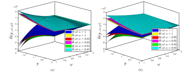
Fig. 2. Comparison of multiple surface profiles of Problem 5.1 established by (a) fuzzy CFD (b) fuzzy ABC fractional derivative operators when different fractional orders correlate with uncertainty factor $\wp$∈[0,1]. |
In Fig. 3 represents the comparison of the lower and upper accuracies between the fuzzy CFD and fuzzy ABC fractional derivative operators for different fractional orders when $\wp$∈[0,1] for expanding hydrologic descriptions at watershed scales.
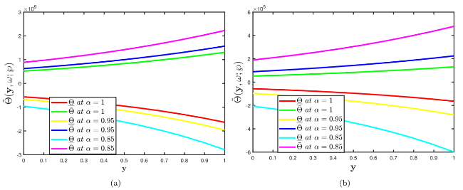
Fig. 3. Comparison of multiple two dimensional profiles of Problem 5.1 established by (a) fuzzy CFD (b) fuzzy ABC fractional derivative operators when different fractional orders correlate with uncertainty factor $\wp$∈[0,1]. |
In Fig. 4 shows the 2D comparison of the upper accuracies between the fuzzy CFD and fuzzy ABC fractional derivative operators when α=0.7. This creates a more conducive environment for analysing spatial relationships between ground topography and water table level.
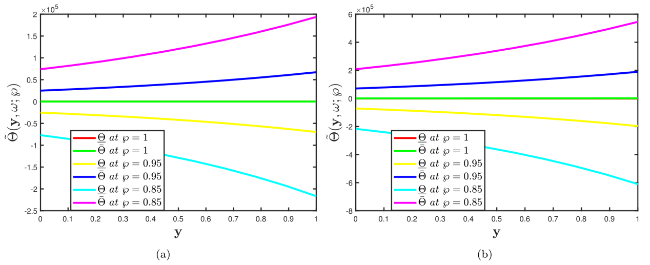
Fig. 4. Comparison of multiple two-dimensional profiles of the Problem 5.1 established by (a) fuzzy CFD (b) fuzzy ABC fractional derivative operators when fractional order α=0.7 correlate with the different uncertainty factors $\wp$∈[0,1]. |
In Fig. 5 gives the surface and 2D comparison by the fuzzy CFD and fuzzy ABC fractional derivative operators that show the interactions between the rainfall and runoff process.
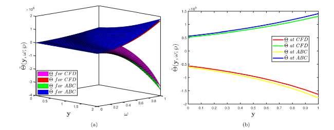
Fig. 5. Comparison of surface profiles (b) Comparison of 2D profiles of Problem 5.1 established by considering fuzzy CFD and fuzzy ABC fractional derivative operators when α=1 and uncertainty factor $\wp$∈[0,1]. |
The important element is that GIADM has provided pairs of solutions for the BSe, which is one of the most significant models in aquifers, with limited computational intricacy and concentration. When the constants in these solutions acquire a particular interpretation, they can be used to describe novel mechanisms of rainfall-runoff curves, irrigation and physical occurrences.
5.2. Fourth-order fuzzy fractional BSe in $\mathbb{R}^{n}$
Problem 5.2. Assume that the generic one-dimensional fourth-order fuzzy fractional BSe is represented as
$\begin{array}{l} \mathscr{D}_{\omega}^{(\alpha)} \widetilde{\Theta}(\overline{\mathbf{y}}, \omega ; \wp)= \sum_{\xi=0}^{n} \eta_{\xi} \odot \mathscr{D}_{\mathbf{y}_{\xi}}^{(4)} \widetilde{\Theta}(\overline{\mathbf{y}}, \omega ; \wp) \\ \oplus \sum_{\xi=0}^{n} \gamma_{\xi} \odot \mathscr{D}_{\mathbf{y}_{\xi}}^{(2)} \widetilde{\Theta}(\overline{\mathbf{y}}, \omega ; \wp) \oplus \sum_{\xi=0}^{n} \Theta_{\xi} \odot \mathscr{D}_{\mathbf{y}_{\xi}}^{(4)} \widetilde{\Theta}^{2}(\overline{\mathbf{y}}, \omega ; \wp) \\ \ominus 4 \sum_{\xi=0}^{n} \Theta_{\xi} \odot \widetilde{\Theta}^{2}(\overline{\mathbf{y}}, \omega ; \wp), \quad \overline{\mathbf{y}}=\left(\mathbf{y}_{1}, \mathbf{y}_{2}, \ldots, \mathbf{y}_{n}\right) \\ \in \mathbb{R}^{n}, \omega>0, \eta_{\xi}, \gamma_{\xi}, \Theta_{\xi} \in \mathbb{R}, \quad(\xi=1,2,., n), \end{array} $
subject to the fuzzy ICs
$\widetilde{\Theta}(\mathbf{y}, 0)=\Upsilon(\wp) \odot \exp \left(\sum_{\xi=0}^{n} \mathbf{y}_{\xi}\right) $
where $\widetilde{\Upsilon}(\wp)=[\underline{\Upsilon}(\wp), \bar{\Upsilon}(\wp)]=[\wp-1,1-\wp] $ for $\wp$∈[0,1] is fuzzy number.
The parameterized version of (5.12) is presented as
$\left\{\begin{array}{l} \mathscr{D}_{\omega}^{(\alpha)} \underline{\Theta}(\mathbf{y}, \omega ; \wp)=\sum_{\xi=0}^{n} \eta_{\xi} \mathscr{D}_{\mathbf{y}_{\xi}}^{(4)} \underline{\Theta}(\overline{\mathbf{y}}, \omega ; \wp)+\sum_{\xi=0}^{n} \gamma_{\xi} \mathscr{D}_{\mathbf{y}_{\xi}}^{(2)} \underline{\Theta}(\overline{\mathbf{y}}, \omega ; \wp)+ \\ \sum_{\xi=0}^{n} \Theta_{\xi} \mathscr{D}_{\mathbf{y}}^{(4)} \underline{\Theta}^{2}(\overline{\mathbf{y}}, \omega ; \wp) \\ \quad-4 \sum_{\xi=0}^{n} \Theta_{\xi} \underline{\Theta}^{2}(\overline{\mathbf{y}}, \omega ; \wp), \\ \underline{\Theta}(\mathbf{y}, 0 ; \wp)=(1-\wp) \exp \left(\sum_{\xi=0}^{n} \mathbf{y}_{\xi}\right), \\ \mathscr{D}_{\omega}^{(\alpha)} \bar{\Theta}(\mathbf{y}, \omega ; \wp)=\sum_{\xi=0}^{n} \eta_{\xi} \mathscr{D}_{\mathbf{y}_{\xi}}^{\left(\mathbf{y}_{\xi}\right)} \bar{\Theta}(\overline{\mathbf{y}}, \omega ; \wp)+\sum_{\xi=0}^{n} \gamma_{\xi} \mathscr{D}_{\mathbf{y}_{\xi}}^{(2)} \bar{\Theta}(\overline{\mathbf{y}}, \omega ; \wp)+ \\ \sum_{\xi=0}^{n} \Theta_{\xi} \mathscr{P}_{y_{\xi}}^{(4)} \bar{\Theta}^{2}(\overline{\mathbf{y}}, \omega ; \wp) \\ \quad-4 \sum_{\xi=0}^{n} \Theta_{\xi} \bar{\Theta}^{2}(\overline{\mathbf{y}}, \omega ; \wp), \\ \bar{\Theta}(\mathbf{y}, 0 ; \wp)=(\wp-1) \exp \left(\sum_{\xi=0}^{n} \mathbf{y}_{\xi}\right). \end{array}\right. $
Case I. Firstly, we apply the generalized integral transform coupled with the $g \mathscr{H}$-differentiability under the Caputo fractional derivative operator to the first case of (5.14).
Employing generalized integral transform to the first preceding case of (5.14), we have
$\begin{aligned} \mathbb{J}\left[\mathscr{D}_{\omega}^{(\alpha)} \underline{\Theta}(\mathbf{y}, \omega ; \wp)\right]= & \mathbb{J}\left[\sum_{\xi=0}^{n} \eta_{\xi} \mathscr{D}_{\mathbf{y}_{\xi}}^{(4)} \underline{\Theta}(\overline{\mathbf{y}}, \omega ; \wp)\right. \\ & +\sum_{\xi=0}^{n} \gamma_{\xi} \mathscr{D}_{\mathbf{y}_{\xi}}^{(2)} \underline{\Theta}(\overline{\mathbf{y}}, \omega ; \wp) \\ + & \sum_{\xi=0}^{n} \Theta_{\xi} \mathscr{D}_{\mathbf{y}_{\xi}}^{(4)} \underline{\Theta}^{2}(\overline{\mathbf{y}}, \omega ; \wp) \\ & \left.-4 \sum_{\xi=0}^{n} \Theta_{\xi} \underline{\Theta}^{2}(\overline{\mathbf{y}}, \omega ; \wp)\right] \end{aligned}$
subject to the IC $\underline{\Theta}(\mathbf{y}, 0)=\exp (\mathbf{y})$, we have
$\begin{array}{l} \Phi^{\alpha}(\varrho) \underline{\mathscr{U}}(\mathbf{y}, \varrho ; \wp)-\Psi(\varrho) \sum_{\kappa=0}^{q-1} \Phi^{\alpha-1-\kappa}(\varrho) \underline{\Theta}^{(\kappa)}(\mathbf{y}, 0 ; \wp) \\ =\mathbb{J}\left[\sum_{\xi=0}^{n} \eta_{\xi} \mathscr{D}_{\mathbf{y}_{\xi}}^{(4)} \underline{\Theta}(\overline{\mathbf{y}}, \omega ; \wp)+\sum_{\xi=0}^{n} \gamma_{\xi} \mathscr{D}_{\mathbf{y}_{\xi}}^{(2)} \underline{\Theta}(\overline{\mathbf{y}}, \omega ; \wp)+\sum_{\xi=0}^{n} \Theta_{\xi} \mathscr{D}_{\mathbf{y}_{\xi}}^{(4)} \underline{\Theta}^{2}(\overline{\mathbf{y}}, \omega ; \wp)\right. \\ \left.-4 \sum_{\xi=0}^{n} \Theta_{\xi} \underline{\Theta}^{2}(\overline{\mathbf{y}}, \omega ; \wp)\right]. \\ \end{array}$
or accordingly, we have
$\begin{aligned} \mathbb{J}[\mathscr{U}(\mathbf{y}, \varrho ; \wp)]= & (\wp-1) \frac{\Psi(\varrho)}{\Phi(\varrho)} \exp \left(\sum_{\xi=0}^{n} \mathbf{y}_{\xi}\right) \\ & +\frac{1}{\Phi^{\alpha}(\varrho)} \mathbb{J}\left[\sum_{\xi=0}^{n} \eta_{\xi} \mathscr{P}_{\mathbf{y}_{\xi}}^{(4)} \underline{\Theta}(\overline{\mathbf{y}}, \omega ; \wp)+\sum_{\xi=0}^{n} \gamma_{\xi} \mathscr{D}_{\mathbf{y}_{\xi}}^{(2)} \Theta(\overline{\mathbf{y}}, \omega ; \wp)\right. \\ & +\sum_{\xi=0}^{n} \Theta_{\xi} \mathscr{D}_{\mathbf{y}_{\xi}}^{(4)} \underline{\Theta}^{2}(\overline{\mathbf{y}}, \omega ; \wp) \\ & \left.-4 \sum_{\xi=0}^{n} \Theta_{\xi} \Theta^{2}(\overline{\mathbf{y}}, \omega ; \wp)\right] \end{aligned}$
The unknown series solution is expressed as
$\underline{\Theta}(\overline{\mathbf{y}}, \omega ; \wp)=\sum_{q=0}^{\infty} \underline{\Theta}(\overline{\mathbf{y}}, \omega ; \wp), $
and the nonlinearity factors are handled as
$\mathscr{N}(\overline{\mathbf{y}}, \omega ; \wp)=\sum_{q=0}^{\infty} \mathscr{A}_{q}(\overline{\mathbf{y}}, \omega ; \wp), $
where $\mathscr{A}_{q}=\underline{\Theta}_{\overline{\mathbf{y}} \overline{\mathbf{y} \bar{y} \bar{y}}}^{2}$ and $\mathscr{B}_{q}=\underline{\Theta}^{2}$ are the Adomian polynomials that can be calculated by the formula (4.8).
Plugging (5.16) and (5.17) into (5.15) can be expressed as
$\begin{aligned} \mathbb{J}\left[\sum_{q=0}^{\infty} \underline{\Theta}(\overline{\mathbf{y}}, \omega ; \wp)\right]= & (\wp-1) \frac{\Psi(\varrho)}{\Phi(\varrho)} \exp \left(\sum_{\xi=0}^{n} \mathbf{y} \xi\right)+\frac{1}{\Phi^{\alpha}(\varrho)} \\ & \times \mathbb{J}\left[\sum_{\xi=0}^{n} \eta_{\xi}\left(\sum_{q=0}^{\infty} \underline{\Theta}_{q}(\overline{\mathbf{y}}, \omega ; \wp)\right) \overline{\mathbf{y} \bar{y} \bar{y}}+\sum_{\xi=0}^{n} \gamma_{\xi}\left(\sum_{q=0}^{\infty} \underline{\Theta}_{q}(\overline{\mathbf{y}}, \omega ; \wp)\right) \overline{\mathbf{y}} \bar{y}\right. \\ & \left.+\sum_{\xi=0}^{n} \Theta_{\xi}\left(\sum_{q=0}^{\infty} \underline{A}_{q}^{2}(\underline{\Theta})\right) \overline{\mathbf{y} \bar{y} \bar{y}}-4 \sum_{\xi=0}^{n} \Theta_{\xi} \sum_{q=0}^{\infty} \underline{B}_{q}(\underline{\Theta})\right]. \end{aligned}$
Applying the inverse generalized integral transform and equating terms on both sides of (5.18), we calculate the following iterative terms by fuzzy CFD fractonal derivative operator as follows:
$\begin{aligned} \underline{\Theta}_{0}(\overline{\mathbf{y}}, \omega ; \wp)= & \mathbb{J}^{-1}\left[(\wp-1) \frac{\Psi(\varrho)}{\Phi(\varrho)} \exp \left(\sum_{\xi=0}^{n} \mathbf{y}_{\xi}\right)\right]=(\wp-1) \exp \left(\sum_{\xi=0}^{n} \mathbf{y}_{\xi}\right), \\ \underline{\Theta}_{1}(\overline{\mathbf{y}}, \omega ; \wp)= & \mathbb{J}^{-1}\left[\frac { 1 } { \Phi ^ { \alpha } ( \varrho ) } \mathbb { J } \left[\sum_{\xi=0}^{n} \eta_{\xi}\left(\underline{\Theta}_{0}(\overline{\mathbf{y}}, \omega ; \wp)\right) \overline{\mathbf{y} \bar{y} \bar{y}}+\sum_{\xi=0}^{n} \gamma_{\xi}\left(\underline{\Theta}_{0}(\overline{\mathbf{y}}, \omega ; \wp)\right) \overline{\mathbf{y} \mathbf{y}}\right.\right. \\ & \left.\left.+\sum_{\xi=0}^{n} \Theta_{\xi}\left(\underline{A}_{0}^{2}(\underline{\Theta})\right) \overline{\mathbf{y} \bar{y} \bar{y}}-4 \sum_{\xi=0}^{n} \Theta_{\xi} \underline{B}_{0}(\underline{\Theta})\right]\right] \\ = & {\left[(\wp-1) \exp \left(\sum_{\xi=0}^{n} \mathbf{y}_{\xi}\right)\left(\sum_{\xi=0}^{n} \eta_{\xi}+\sum_{\xi=0}^{n} \gamma_{\xi}\right)\right.} \\ & \left.+4 \sum_{\xi=0}^{n} \Theta_{\xi}(\wp-1)^{2} \exp \left(2 \sum_{\xi=0}^{n} \mathbf{y}_{\xi}\right)\right] \frac{\omega^{\alpha}}{\Gamma(\alpha+1)}, \end{aligned}$
$\begin{aligned} \underline{\Theta}_{2}(\overline{\mathbf{y}}, \omega ; \wp)= & \mathbb{J}^{-1}\left[\frac { 1 } { \Phi ^ { \alpha } ( \varrho ) } \mathbb { J } \left[\sum_{\xi=0}^{n} \eta_{\xi}\left(\underline{\Theta}_{1}(\overline{\mathbf{y}}, \omega ; \wp)\right) \overline{\bar{y} \bar{y} \bar{y}}+\sum_{\xi=0}^{n} \gamma_{\xi}\left(\underline{\Theta}_{1}(\overline{\mathbf{y}}, \omega ; \wp)\right) \overline{\bar{y} \bar{y}}\right.\right. \\ & +\sum_{\xi=0}^{n} \Theta_{\xi}\left(\underline{A}_{1}^{2}(\underline{\Theta})\right) \overline{\bar{y} \bar{y} \bar{y}} \\ & \left.\left.-4 \sum_{\xi=0}^{n} \Theta_{\xi} \underline{B}_{1}(\underline{\Theta})\right]\right] \\ = & {\left[\exp \left(\sum_{\xi=0}^{n} \mathbf{y}_{\xi}\right)\left(\sum_{\xi=0}^{n} \eta_{\xi}+\sum_{\xi=0}^{n} \gamma_{\xi}\right)^{2}(\wp-1)\right.} \\ & +2\left(1-4 \sum_{\xi=0}^{n} \Theta_{\xi}\right) \exp \left(2 \sum_{\xi=0}^{n} \mathbf{y}_{\xi}\right)(\wp-1)^{2} \\ & \times\left(\sum_{\xi=0}^{n} \eta_{\xi}+\sum_{\xi=0}^{n} \gamma_{\xi}\right)+8 \sum_{\xi=0}^{n} \Theta_{\xi}(\wp-1)^{3}\left(1-\sum_{\xi=0}^{n} \Theta_{\xi}\right) \\ & \left.\exp \left(3 \sum_{\xi=0}^{n} \mathbf{y}_{\xi}\right)\right] \frac{\omega^{2 \alpha}}{\Gamma(2 \alpha+1)}. \end{aligned}$
Thus, the desired approximate solution is written as
$\widetilde{\Theta}(\overline{\mathbf{y}}, \omega ; \wp)=\widetilde{\Theta}_{0}(\overline{\mathbf{y}}, \omega ; \wp)+\widetilde{\Theta}_{1}(\overline{\mathbf{y}}, \omega ; \wp)+\ldots, $
implies that
$\begin{aligned} \underline{\Theta} & (\overline{\mathbf{y}}, \omega ; \wp)=\underline{\Theta}_{0}(\overline{\mathbf{y}}, \omega ; \wp)+\underline{\Theta}_{1}(\overline{\mathbf{y}}, \omega ; \wp)+\ldots \\ = & (\wp-1) \exp \left(\sum_{\xi=0}^{n} \mathbf{y}_{\xi}\right)+\left[(\wp-1) \exp \left(\sum_{\xi=0}^{n} \mathbf{y}_{\xi}\right)\left(\sum_{\xi=0}^{n} \eta_{\xi}+\sum_{\xi=0}^{n} \gamma_{\xi}\right)\right. \\ & \left.+4 \sum_{\xi=0}^{n} \Theta_{\xi}(\wp-1)^{2} \exp \left(2 \sum_{\xi=0}^{n} \mathbf{y}_{\xi}\right)\right] \frac{\omega^{\alpha}}{\Gamma(\alpha+1)} \\ & +\left[\exp \left(\sum_{\xi=0}^{n} \mathbf{y}_{\xi}\right)\left(\sum_{\xi=0}^{n} \eta_{\xi}+\sum_{\xi=0}^{n} \gamma_{\xi}\right)^{2}(\wp-1)\right. \\ + & 2\left(1-4 \sum_{\xi=0}^{n} \Theta_{\xi}\right) \exp \left(2 \sum_{\xi=0}^{n} \mathbf{y}_{\xi}\right)(\wp-1)^{2} \\ & \left.\times\left(\sum_{\xi=0}^{n} \eta_{\xi}+\sum_{\xi=0}^{n} \gamma_{\xi}\right)+8 \sum_{\xi=0}^{n} \Theta_{\xi}(\wp-1)^{3}\left(1-\sum_{\xi=0}^{n} \Theta_{\xi}\right) \exp \left(3 \sum_{\xi=0}^{n} \mathbf{y}_{\xi}\right)\right] \frac{\omega^{2 \alpha}}{\Gamma(2 \alpha+1)} \\ + & \ldots, \end{aligned}$
$\begin{aligned} \bar{\Theta} & (\overline{\mathbf{y}}, \omega ; \wp)=\bar{\Theta}_{0}(\overline{\mathbf{y}}, \omega ; \wp)+\bar{\Theta}_{1}(\overline{\mathbf{y}}, \omega ; \wp)+\ldots \\ = & (1-\wp) \exp \left(\sum_{\xi=0}^{n} \mathbf{y}_{\xi}\right)+\left[(1-\wp) \exp \left(\sum_{\xi=0}^{n} \mathbf{y}_{\xi}\right)\left(\sum_{\xi=0}^{n} \eta_{\xi}+\sum_{\xi=0}^{n} \gamma_{\xi}\right)\right. \\ & \left.+4 \sum_{\xi=0}^{n} \Theta_{\xi}(1-\wp)^{2} \exp \left(2 \sum_{\xi=0}^{n} \mathbf{y}_{\xi}\right)\right] \frac{\omega^{\alpha}}{\Gamma(\alpha+1)} \\ & +\left[\exp \left(\sum_{\xi=0}^{n} \mathbf{y}_{\xi}\right)\left(\sum_{\xi=0}^{n} \eta_{\xi}+\sum_{\xi=0}^{n} \gamma_{\xi}\right)^{2}(1-\wp)\right. \\ + & 2\left(1-4 \sum_{\xi=0}^{n} \Theta_{\xi}\right) \exp \left(2 \sum_{\xi=0}^{n} \mathbf{y}_{\xi}\right)(1-\wp)^{2} \\ & \left.\times\left(\sum_{\xi=0}^{n} \eta_{\xi}+\sum_{\xi=0}^{n} \gamma_{\xi}\right)+8 \sum_{\xi=0}^{n} \Theta_{\xi}(1-\wp)^{3}\left(1-\sum_{\xi=0}^{n} \Theta_{\xi}\right) \exp \left(3 \sum_{\xi=0}^{n} \mathbf{y}_{\xi}\right)\right] \frac{\omega^{2 \alpha}}{\Gamma(2 \alpha+1)} \\ & +\ldots \end{aligned}$
Case II. Now, we apply the generalized integral transform coupled with the $g \mathscr{H}$-differentiability under the ABC fractional derivative to the first case of (5.14).
Also, the transformed function in the fuzzy ABC derivative sense
$\begin{aligned} & \frac{\Phi^{\alpha}(\varrho) \mathbb{B}(\alpha)}{\alpha+(1-\alpha) \Phi^{\alpha}(s)}\left[\underline{\mathscr{U}}(\overline{\mathbf{y}}, \varrho ; \wp)-\frac{\Psi(\varrho)}{\Phi(s)} \underline{\Theta}(\overline{\mathbf{y}}, 0 ; \wp)\right] \\ = & \mathbb{J}\left[\sum_{\xi=0}^{n} \eta_{\xi} \mathscr{D}_{\mathbf{y}_{\xi}}^{(4)} \underline{\Theta}(\overline{\mathbf{y}}, \omega ; \wp)+\sum_{\xi=0}^{n} \gamma_{\xi} \mathscr{D}_{\mathbf{y}_{\xi}}^{(2)} \underline{\Theta}(\overline{\mathbf{y}}, \omega ; \wp)+\sum_{\xi=0}^{n} \Theta_{\xi} \mathscr{D}_{\mathbf{y}_{\xi}}^{(4)} \underline{\Theta}^{2}(\overline{\mathbf{y}}, \omega ; \wp)\right. \\ & \left.-4 \sum_{\xi=0}^{n} \Theta_{\xi} \underline{\Theta}^{2}(\overline{\mathbf{y}}, \omega ; \wp)\right], \end{aligned}$
or accordingly, we have
$\begin{aligned} \mathbb{J}[\mathscr{U}(\overline{\mathbf{y}}, \varrho ; \wp)]= & (\wp-1) \frac{\Psi(\varrho)}{\Phi(\varrho)} \exp \left(\sum_{\xi=0}^{n} \mathbf{y}_{\xi}\right)+\left(\frac{\alpha+(1-\alpha) \Phi^{\alpha}(\varrho)}{\Phi^{\alpha}(\varrho) \mathbb{B}(\alpha)}\right) \\ & \times \mathbb{J}\left[\sum_{\xi=0}^{n} \eta_{\xi} \mathscr{D}_{\mathbf{y}_{\xi}}^{(4)} \underline{\Theta}(\overline{\mathbf{y}}, \omega ; \wp)+\sum_{\xi=0}^{n} \gamma_{\xi} \mathscr{D}_{\mathbf{y}_{\xi}}^{(2)} \underline{\Theta}(\overline{\mathbf{y}}, \omega ; \wp)\right. \\ & \left.+\sum_{\xi=0}^{n} \Theta_{\xi} \mathscr{D}_{\mathbf{y}_{\xi}}^{(4)} \underline{\Theta}^{2}(\overline{\mathbf{y}}, \omega ; \wp)-4 \sum_{\xi=0}^{n} \Theta_{\xi} \underline{\Theta}^{2}(\overline{\mathbf{y}}, \omega ; \wp)\right]. \end{aligned}$
The unknown series solution is expressed as
$\underline{\Theta}(\overline{\mathbf{y}}, \omega ; \wp)=\sum_{q=0}^{\infty} \underline{\Theta}(\overline{\mathbf{y}}, \omega ; \wp), $
and the nonlinearity factors are handled as
$\mathscr{N}(\overline{\mathbf{y}}, \omega ; \wp)=\sum_{q=0}^{\infty} \underline{\mathscr{A}}_{q}(\overline{\mathbf{y}}, \omega ; \wp) $
where $\mathscr{A}_{q}=\underline{\Theta}_{\text {уууу }}^{2}$ and $\mathscr{B}_{q}=\underline{\Theta}^{2}$ are the Adomian polynomials that can be calculated by the formula (4.8).
Now, plugging (5.20) and (5.21) into (5.19), then we have
$\begin{aligned} \mathbb{J}\left[\sum_{q=0}^{\infty} \underline{\Theta}(\overline{\mathbf{y}}, \omega ; \wp)\right]= & (\wp-1) \frac{\Psi(\varrho)}{\Phi(\varrho)} \exp \left(\sum_{\xi=0}^{n} \mathbf{y}_{\xi}\right)+\left(\frac{\alpha+(1-\alpha) \Phi^{\alpha}(\varrho)}{\Phi^{\alpha}(\varrho) \mathbb{B}(\alpha)}\right) \\ & \times \mathbb{J}\left[\sum_{\xi=0}^{n} \eta_{\xi}\left(\sum_{q=0}^{\infty} \underline{\Theta}_{q}(\overline{\mathbf{y}}, \omega ; \wp)\right) \overline{y y y y}+\sum_{\xi=0}^{n} \gamma_{\xi}\left(\sum_{q=0}^{\infty} \underline{\Theta}_{q}(\overline{\mathbf{y}}, \omega ; \wp)\right) \overline{y y}\right. \\ & \left.+\sum_{\xi=0}^{n} \Theta_{\xi}\left(\sum_{q=0}^{\infty} \underline{A}_{q}^{2}(\underline{\Theta})\right) \overline{\bar{y} \bar{y} \bar{y}}-4 \sum_{\xi=0}^{n} \Theta_{\xi} \sum_{q=0}^{\infty} \underline{B}_{q}(\underline{\Theta})\right] \end{aligned}$
Applying the inverse generalized integral transform and equating terms on both sides of (5.22), we calculate the following iterative terms by the fuzzy AB fractonal derivative operator in the Caputo sense:
$\begin{aligned} \underline{\Theta}_{1}(\overline{\mathbf{y}}, \omega ; \wp)= & \mathbb{J}^{-1}\left[(\wp-1) \frac{\Psi(\varrho)}{\Phi(\varrho)} \exp \left(\sum_{\xi=0}^{n} \mathbf{y}_{\xi}\right)\right]=(\wp-1) \exp \left(\sum_{\xi=0}^{n} \mathbf{y}_{\xi}\right), \\ \underline{\Theta}_{1}(\overline{\mathbf{y}}, \omega ; \wp)= & \mathbb{J}^{-1}\left[( \frac { \alpha + ( 1 - \alpha ) \Phi ^ { \alpha } ( \varrho ) } { \Phi ^ { \alpha } ( \varrho ) \mathbb { B } ( \alpha ) } ) \mathbb { J } \left[\sum_{\xi=0}^{n} \eta_{\xi}\left(\underline{\Theta}_{0}(\overline{\mathbf{y}}, \omega ; \wp)\right) \overline{\mathbf{y} \bar{y} \bar{y} \bar{y}}\right.\right. \\ & \left.\left.+\sum_{\xi=0}^{n} \gamma_{\xi}\left(\underline{\Theta}_{0}(\overline{\mathbf{y}}, \omega ; \wp)\right) \overline{\bar{y} \bar{y}}+\sum_{\xi=0}^{n} \Theta_{\xi}\left(\underline{A}_{0}^{2}(\underline{\Theta})\right) \bar{y}_{\bar{y} \bar{y} \bar{y}}-4 \sum_{\xi=0}^{n} \Theta_{\xi} \underline{B}_{0}(\underline{\Theta})\right]\right] \\ = & {\left[(\wp-1) \exp \left(\sum_{\xi=0}^{n} \mathbf{y}_{\xi}\right)\left(\sum_{\xi=0}^{n} \eta_{\xi}+\sum_{\xi=0}^{n} \gamma_{\xi}\right)+4 \sum_{\xi=0}^{n} \Theta_{\xi}(\wp-1)^{2}\right.} \\ & \left.\exp \left(2 \sum_{\xi=0}^{n} \mathbf{y}_{\xi}\right)\right]\left(\frac{\alpha \omega^{\alpha}}{\Gamma(\alpha+1)}+(1-\alpha)\right), \end{aligned}$
$\begin{aligned} \underline{\Theta}_{2}(\overline{\mathbf{y}}, \omega ; \wp)= & \mathbb{J}^{-1}\left[( \frac { \alpha + ( 1 - \alpha ) \Phi ^ { \alpha } ( \varrho ) } { \Phi ^ { \alpha } ( \varrho ) \mathbb { B } ( \alpha ) } ) \mathbb { J } \left[\sum_{\xi=0}^{n} \eta_{\xi}\left(\underline{\Theta}_{1}(\overline{\mathbf{y}}, \omega ; \wp)\right) \overline{\bar{y} \bar{y} \bar{y}}\right.\right. \\ + & \sum_{\xi=0}^{n} \gamma_{\xi}\left(\underline{\Theta}_{1}(\overline{\mathbf{y}}, \omega ; \wp)\right) \overline{\mathbf{y} \bar{y}} \\ & \left.\left.+\sum_{\xi=0}^{n} \Theta_{\xi}\left(\underline{A}_{1}^{2}(\underline{\Theta})\right) \overline{\mathbf{y} \bar{y} \bar{y} \bar{y}}-4 \sum_{\xi=0}^{n} \Theta_{\xi} \underline{B}_{1}(\underline{\Theta})\right]\right] \\ = & {\left[\exp \left(\sum_{\xi=0}^{n} \mathbf{y}_{\xi}\right)\left(\sum_{\xi=0}^{n} \eta_{\xi}+\sum_{\xi=0}^{n} \gamma_{\xi}\right)^{2}(\wp-1)+2\left(1-4 \sum_{\xi=0}^{n} \Theta_{\xi}\right)\right.} \\ & \exp \left(2 \sum_{\xi=0}^{n} \mathbf{y}_{\xi}\right)(\wp-1)^{2}\left(\sum_{\xi=0}^{n} \eta_{\xi}+\sum_{\xi=0}^{n} \gamma_{\xi}\right) \\ & \left.+8 \sum_{\xi=0}^{n} \Theta_{\xi}(\wp-1)^{3}\left(1-\sum_{\xi=0}^{n} \Theta_{\xi}\right) \exp \left(3 \sum_{\xi=0}^{n} \mathbf{y}_{\xi}\right)\right] \\ & \times\left(\frac{\alpha^{2} \omega^{2 \alpha}}{\Gamma(2 \alpha+1)}+2 \alpha(1-\alpha) \frac{\omega^{\alpha}}{\Gamma(1+\alpha)}+(1-\alpha)^{2}\right). \end{aligned}$
Thus, the desired approximate solution is written as
$\widetilde{\Theta}(\overline{\mathbf{y}}, \omega ; \wp)=\widetilde{\Theta}_{0}(\overline{\mathbf{y}}, \omega ; \wp)+\widetilde{\Theta}_{1}(\overline{\mathbf{y}}, \omega ; \wp)+\ldots, $
implies that
$\begin{aligned} \underline{\Theta}(\overline{\mathbf{y}}, \omega ; \wp)= & \underline{\Theta}_{0}(\overline{\mathbf{y}}, \omega ; \wp)+\underline{\Theta}_{1}(\overline{\mathbf{y}}, \omega ; \wp)+\ldots \\ = & (\wp-1) \exp \left(\sum_{\xi=0}^{n} \mathbf{y}_{\xi}\right)+\left[(\wp-1) \exp \left(\sum_{\xi=0}^{n} \mathbf{y}_{\xi}\right)\left(\sum_{\xi=0}^{n} \eta_{\xi}+\sum_{\xi=0}^{n} \gamma_{\xi}\right)\right. \\ + & \left.4 \sum_{\xi=0}^{n} \Theta_{\xi}(\wp-1)^{2} \exp \left(2 \sum_{\xi=0}^{n} \mathbf{y}_{\xi}\right)\right] \\ & \times\left(\frac{\alpha \omega^{\alpha}}{\Gamma(\alpha+1)}+(1-\alpha)\right)+\left[\exp \left(\sum_{\xi=0}^{n} \mathbf{y}_{\xi}\right)\left(\sum_{\xi=0}^{n} \eta_{\xi}+\sum_{\xi=0}^{n} \gamma_{\xi}\right)^{2}(\wp-1)\right. \\ & +2\left(1-4 \sum_{\xi=0}^{n} \Theta_{\xi}\right) \exp \left(2 \sum_{\xi=0}^{n} \mathbf{y}_{\xi}\right)(\wp-1)^{2}\left(\sum_{\xi=0}^{n} \eta_{\xi}+\sum_{\xi=0}^{n} \gamma_{\xi}\right) \\ & \left.+8 \sum_{\xi=0}^{n} \Theta_{\xi}(\wp-1)^{3}\left(1-\sum_{\xi=0}^{n} \Theta_{\xi}\right) \exp \left(3 \sum_{\xi=0}^{n} \mathbf{y}_{\xi}\right)\right] \\ & \times\left(\frac{\alpha^{2} \omega^{2 \alpha}}{\Gamma(2 \alpha+1)}+2 \alpha(1-\alpha) \frac{\omega^{\alpha}}{\Gamma(1+\alpha)}+(1-\alpha)^{2}\right)+\ldots, \end{aligned}$
$\begin{aligned} \bar{\Theta}(\overline{\mathbf{y}}, \omega ; \wp)= & \bar{\Theta}_{0}(\overline{\mathbf{y}}, \omega ; \wp)+\bar{\Theta}_{1}(\overline{\mathbf{y}}, \omega ; \wp)+\ldots \\ = & (1-\wp) \exp \left(\sum_{\xi=0}^{n} \mathbf{y}_{\xi}\right)+\left[(1-\wp) \exp \left(\sum_{\xi=0}^{n} \mathbf{y}_{\xi}\right)\left(\sum_{\xi=0}^{n} \eta_{\xi}+\sum_{\xi=0}^{n} \gamma_{\xi}\right)\right. \\ + & \left.4 \sum_{\xi=0}^{n} \Theta_{\xi}(1-\wp)^{2} \exp \left(2 \sum_{\xi=0}^{n} \mathbf{y}_{\xi}\right)\right] \\ & \times\left(\frac{\alpha \omega^{\alpha}}{\Gamma(\alpha+1)}+(1-\alpha)\right)+\left[\exp \left(\sum_{\xi=0}^{n} \mathbf{y}_{\xi}\right)\left(\sum_{\xi=0}^{n} \eta_{\xi}+\sum_{\xi=0}^{n} \gamma_{\xi}\right)^{2}(1-\wp)\right. \\ & +2\left(1-4 \sum_{\xi=0}^{n} \Theta_{\xi}\right) \exp \left(2 \sum_{\xi=0}^{n} \mathbf{y}_{\xi}\right)(1-\wp)^{2}\left(\sum_{\xi=0}^{n} \eta_{\xi}+\sum_{\xi=0}^{n} \gamma_{\xi}\right) \\ & \left.+8 \sum_{\xi=0}^{n} \Theta_{\xi}(1-\wp)^{3}\left(1-\sum_{\xi=0}^{n} \Theta_{\xi}\right) \exp \left(3 \sum_{\xi=0}^{n} \mathbf{y}_{\xi}\right)\right] \\ & \times\left(\frac{\alpha^{2} \omega^{2 \alpha}}{\Gamma(2 \alpha+1)}+2 \alpha(1-\alpha) \frac{\omega^{\alpha}}{\Gamma(1+\alpha)}+(1-\alpha)^{2}\right)+\ldots \end{aligned}$
Fig. 6 illustrates the three-dimensional comparison between the lower and upper solutions of $\widetilde{\Theta}(\mathbf{y}, \omega ; \wp) $ for Problem 5.2 when α=1 and uncertainty factor $\wp$∈[0,1] by means of $g \mathscr{H}$-differentiability of Caputo and ABC fractional derivative subject to fuzzy ICs when real constants are η=10, γ=20 and θ=5. The GIADM solution exhibits a strong correlation with both fractional-order derivatives.
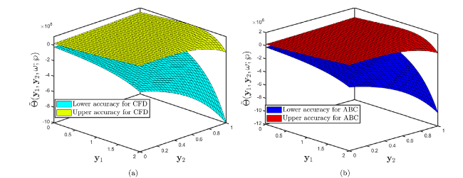
Fig. 6. Comparison of 3D surface profile of Problem 5.2 established by (a) fuzzy CFD (b) fuzzy ABC fractional derivative operators when α=1 and uncertainty factor $\wp$∈[0,1]. |
From Fig. 7, (a and b) Comparison of multiple surface plots for different fractional orders with the fuzzy fractional CFD and ABC derivative operators are presented. Furthermore, it can be shown that by increasing the realistic representation of stream flow and groundwater dynamics on hillslopes in the plasma at $\wp$=.7.
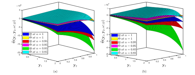
Fig. 7. Comparison of multiple surface profiles of Problem 5.2 established by (a) fuzzy CFD (b) fuzzy ABC fractional derivative operators when different fractional orders correlate with uncertainty factor $\wp$∈[0,1]. |
In Fig. 8 represents the comparison of the lower and upper accuracies between the fuzzy CFD and fuzzy ABC fractional derivative operators for different fractional orders when $\wp$∈[0,1] for expanding hydrologic descriptions at watershed scales.
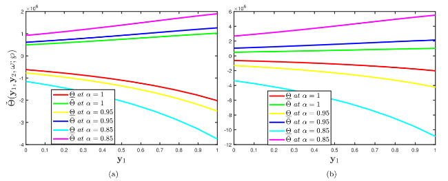
Fig. 8. Comparison of multiple two dimensional profiles of Problem 5.2 established by (a) fuzzy CFD (b) fuzzy ABC fractional derivative operators when different fractional orders correlate with uncertainty factor $\wp$∈[0,1]. |
In Fig. 9 shows the 2D comparison of the upper accuracies between the fuzzy CFD and fuzzy ABC fractional derivative operators when α=0.7. This creates a more conducive environment for analysing spatial relationships between ground topography and water table level.
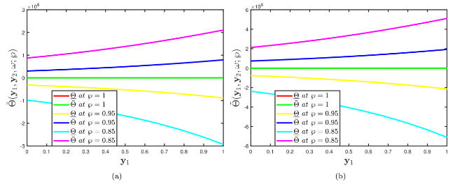
Fig. 9. Comparison of multiple two-dimensional profiles of the Problem 5.2 established by (a) fuzzy CFD (b) fuzzy ABC fractional derivative operators when fractional order α=0.7 correlate with the different uncertainty factors $\wp$∈[0,1]. |
In Fig. 10 gives the surface and 2D comparison by the fuzzy CFD and fuzzy ABC fractional derivative operators that show the interactions between the rainfall and runoff process.
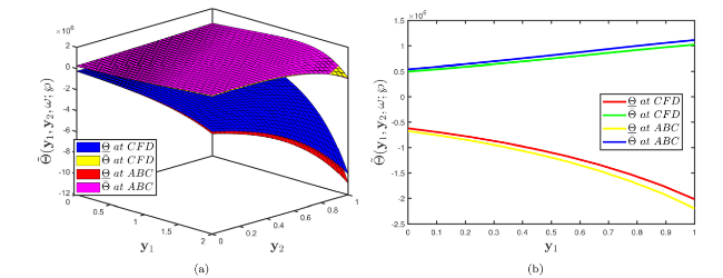
Fig. 10. (a) Comparison of surface profiles (b) Comparison of 2D profiles of Problem 5.2 established by fuzzy CFD and fuzzy ABC fractional derivative operators when α=1 and uncertainty factor $\wp$∈[0,1]. |
The important element is that GIADM has provided pairs of solutions for the BSe, which is one of the most significant models in aquifers, with limited computational intricacy and concentration. When the constants in these solutions acquire a particular interpretation, they can be used to describe novel mechanisms of rainfall-runoff curves, irrigation and physical occurrences.
5.3. (2ndth)-Order fuzzy fractional BSe in $\mathbb{R}$
Problem 5.3. Assume that the generic one-dimensional (2nth)-order fuzzy fractional BSe is represented as
$\begin{aligned} \mathscr{D}_{\omega}^{(\alpha)} \widetilde{\Theta}(\mathbf{y}, \omega ; \wp)= & \mathscr{D}_{\mathbf{y}}^{(2 n)} \widetilde{\Theta}(\mathbf{y}, \omega ; \wp) \oplus \mathscr{D}_{\mathbf{y}}^{(2 n-2)} \widetilde{\Theta}(\mathbf{y}, \omega ; \wp) \oplus \ldots \\ \oplus & \mathscr{D}_{\mathbf{y}}^{(2)} \widetilde{\Theta}(\mathbf{y}, \omega ; \wp) \oplus \Theta \odot \mathscr{D}_{\mathbf{y}}^{(2)} \widetilde{\Theta}^{2}(\mathbf{y}, \omega ; \wp) \\ & \ominus 4 \Theta \odot \underline{\Theta}^{2}(\mathbf{y}, \omega ; \wp), \quad \mathbf{y} \in \mathbb{R}, \omega>0 \end{aligned}$
subject to the fuzzy ICs
$\widetilde{\Theta}(\mathbf{y}, 0)=\Upsilon \odot \exp (\mathbf{y})$
where $\tilde{\Upsilon}(\wp)=[\underline{\Upsilon}(\wp), \bar{\Upsilon}(\wp)]=[\wp-1,1-\wp] $ for $\wp$∈[0,1] is fuzzy number.
The parameterized version of (5.23) is presented as
$\left\{\begin{array}{l} \mathscr{D}_{\omega}^{(\alpha)} \underline{\Theta}(\mathbf{y}, \omega ; \wp)=\mathscr{D}_{\mathbf{y}}^{(2 n)} \underline{\Theta}(\mathbf{y}, \omega ; \wp)+\mathscr{D}_{\mathbf{y}}^{(2 n-2)} \underline{\Theta}(\mathbf{y}, \omega ; \wp)+\ldots+\mathscr{D}_{\mathbf{y}}^{(2)} \underline{\Theta}(\mathbf{y}, \omega ; \wp) \\ \quad+\Theta \mathscr{D}_{\mathbf{y}}^{(2)} \underline{\Theta}^{2}(\mathbf{y}, \omega ; \wp)-4 \Theta \underline{\Theta}^{2}(\mathbf{y}, \omega ; \wp), \\ \underline{\Theta}(\mathbf{y}, 0 ; \wp)=(1-\wp) \exp (\mathbf{y}) \\ \mathscr{D}_{\omega}^{(\alpha)} \bar{\Theta}(\mathbf{y}, \omega ; \wp)=\mathscr{D}_{\mathbf{y}}^{(2 n)} \bar{\Theta}(\mathbf{y}, \omega ; \wp)+\mathscr{D}_{\mathbf{y}}^{(2 n-2)} \bar{\Theta}(\mathbf{y}, \omega ; \wp)+\ldots \\ +\mathscr{D}_{\mathbf{y}}^{(2)} \bar{\Theta}(\mathbf{y}, \omega ; \wp) \\ \quad+\Theta \mathscr{D}_{\mathbf{y}}^{(2)} \bar{\Theta}^{2}(\mathbf{y}, \omega ; \wp)-4 \Theta \bar{\Theta}^{2}(\mathbf{y}, \omega ; \wp), \\ \bar{\Theta}(\mathbf{y}, 0 ; \wp)=(\wp-1) \exp (\mathbf{y}). \end{array}\right. $
Case I. Firstly, we apply the generalized integral transform coupled with the $g \mathscr{H}$ differentiability under the Caputo fractional derivative operator to the first case of (5.25).
Employing generalized integral transform to the first preceding case of (5.25), we have
$\begin{aligned} \mathbb{J}\left[\mathscr{D}_{\omega}^{(\alpha)} \underline{\Theta}(\mathbf{y}, \omega ; \wp)\right] \quad & =\mathbb{J}\left[\mathscr{D}_{\mathbf{y}}^{(2 n)} \underline{\Theta}(\mathbf{y}, \omega ; \wp)+\mathscr{D}_{\mathbf{y}}^{(2 n-2)} \underline{\Theta}(\mathbf{y}, \omega ; \wp)+\ldots\right. \\ & \left.+\mathscr{D}_{\mathbf{y}}^{(2)} \underline{\Theta}(\mathbf{y}, \omega ; \wp)+\Theta \mathscr{D}_{\mathbf{y}}^{(2)} \underline{\Theta}^{2}(\mathbf{y}, \omega ; \wp)\right] \end{aligned}$
subject to the IC $\underline{\Theta}(\mathbf{y}, 0)=\exp (\mathbf{y})$, we have
$\begin{array}{l} \Phi^{\alpha}(\varrho) \underline{\mathscr{U}}(\mathbf{y}, \varrho ; \wp)-\Psi(\varrho) \sum_{\kappa=0}^{q-1} \Phi^{\alpha-1-\kappa}(\varrho) \underline{\Theta}^{(\kappa)}(\mathbf{y}, 0 ; \wp) \\ =\mathbb{J}\left[\mathscr{D}_{\mathbf{y}}^{(2 n)} \underline{\Theta}(\mathbf{y}, \omega ; \wp)+\mathscr{D}_{\mathbf{y}}^{(2 n-2)} \underline{\Theta}(\mathbf{y}, \omega ; \wp)+\ldots\right. \\ \left.+\mathscr{D}_{\mathbf{y}}^{(2)} \underline{\Theta}(\mathbf{y}, \omega ; \wp)+\Theta \mathscr{D}_{\mathbf{y}}^{(2)} \underline{\Theta}^{2}(\mathbf{y}, \omega ; \wp)\right]. \end{array}$
or accordingly, we have
$\begin{aligned} \mathbb{J}[\mathscr{U}(\mathbf{y}, \varrho ; \wp)]= & (\wp-1) \frac{\Psi(\varrho)}{\Phi(\varrho)} \exp (\mathbf{y}) \\ & +\frac{1}{\Phi^{\alpha}(\varrho)} \mathbb{J}\left[\mathscr{D}_{\mathbf{y}}^{(2 n)} \underline{\Theta}(\mathbf{y}, \omega ; \wp)+\mathscr{D}_{\mathbf{y}}^{(2 n-2)} \underline{\Theta}(\mathbf{y}, \omega ; \wp)\right. \\ & \left.+\ldots+\mathscr{D}_{\mathbf{y}}^{(2)} \underline{\Theta}(\mathbf{y}, \omega ; \wp)+\Theta \mathscr{D}_{\mathbf{y}}^{(2)} \underline{\Theta}^{2}(\mathbf{y}, \omega ; \wp)\right]. \end{aligned}$
The unknown series solution is expressed as
$\underline{\Theta}(\mathbf{y}, \omega ; \wp)=\sum_{q=0}^{\infty} \underline{\Theta}(\mathbf{y}, \omega ; \wp), $
and the nonlinearity factors are handled as
$\underline{\mathscr{N}}(\mathbf{y}, \omega ; \wp)=\sum_{q=0}^{\infty} \mathscr{A}_{q}(\mathbf{y}, \omega ; \wp), $
where $\mathscr{A}_{q}=\underline{\Theta}_{\mathbf{y y y y}}^{2}$ and $\mathscr{B}_{q}=\underline{\Theta}^{2}$ are the Adomian polynomials that can be calculated by the formula (4.8).
Plugging (5.27) and (5.28) into (5.26) can be expressed as
$\begin{aligned} \mathbb{J}\left[\sum_{q=0}^{\infty} \underline{\Theta}(\mathbf{y}, \omega ; \wp)\right]= & (\wp-1) \frac{\Psi(\varrho)}{\Phi(\varrho)} \exp (\mathbf{y})+\frac{1}{\Phi^{\alpha}(\varrho)} \mathbb{J}\left[\left(\sum_{q=0}^{\infty} \underline{\Theta}_{q}(\mathbf{y}, \omega ; \wp)\right)(2 n)_{\mathbf{y}}\right. \\ + & \left(\sum_{q=0}^{\infty} \underline{\Theta}_{q}(\mathbf{y}, \omega ; \wp)\right)(2 n-2)_{y} \\ & +\ldots+\left(\sum_{q=0}^{\infty} \underline{\Theta}_{q}(\mathbf{y}, \omega ; \wp)\right) \mathbf{y}+\Theta\left(\sum_{q=0}^{\infty} \underline{A}_{q}^{2}(\underline{\Theta})\right) \mathbf{y y} \\ - & \left.4 \Theta \sum_{q=0}^{\infty} \underline{B}_{q}(\underline{\Theta})\right]. \end{aligned} $
Applying the inverse generalized integral transform and equating factors on both sides of (5.29), we calculate the following iterative terms by fuzzy CFD fractonal derivative operator as follows:
$\begin{aligned} \underline{\Theta}_{0}(\mathbf{y}, \omega ; \wp)= & \mathbb{J}^{-1}\left[(\wp-1) \frac{\Psi(\varrho)}{\Phi(\varrho)} \exp (\mathbf{y})\right]=(\wp-1) \exp (\mathbf{y}) \\ \underline{\Theta}_{1}(\mathbf{y}, \omega ; \wp)= & \mathbb{J}^{-1}\left[\frac { 1 } { \Phi ^ { \alpha } ( \varrho ) } \mathbb { J } \left[\left(\underline{\Theta}_{0}(\mathbf{y}, \omega ; \wp)\right)_{(2 n) \mathbf{y}}+\left(\underline{\Theta}_{0}(\mathbf{y}, \omega ; \wp)\right)_{(2 n-2) \mathbf{y}}+\ldots+\left(\underline{\Theta}_{0}(\mathbf{y}, \omega ; \wp)\right)_{\mathbf{y}}\right.\right. \\ & \left.\left.+\Theta\left(\underline{A}_{0}^{2}(\underline{\Theta})\right)_{\mathbf{y}}-4 \Theta \underline{B}_{0}(\underline{\Theta})\right]\right] \\ = & {[n(\wp-1) \exp (\mathbf{y})] \frac{\omega^{\alpha}}{\Gamma(\alpha+1)}, } \\ \underline{\Theta}_{2}(\mathbf{y}, \omega ; \wp)= & \mathbb{J}^{-1}\left[\frac { 1 } { \Phi ^ { \alpha } ( \varrho ) } \mathbb { J } \left[\left(\underline{\Theta}_{1}(\mathbf{y}, \omega ; \wp)\right)_{(2 n) \mathbf{y}}+\left(\underline{\Theta}_{1}(\mathbf{y}, \omega ; \wp)\right)_{(2 n-2) \mathbf{y}}+\ldots+\left(\underline{\Theta}_{1}(\mathbf{y}, \omega ; \wp)\right)_{\mathbf{y}}\right.\right. \\ & \left.\left.+\Theta\left(\underline{A}_{1}^{2}(\underline{\Theta})\right)_{\mathbf{y}}-4 \Theta \underline{B}_{1}(\underline{\Theta})\right]\right] \\ = & n \exp (\mathbf{y})(\wp-1)[n+2 \Theta(\wp-1)-8 \Theta(\wp-1) \exp (\mathbf{y})] \frac{\omega^{2 \alpha}}{\Gamma(2 \alpha+1)}. \end{aligned} $
Hence, the required series solution is expressed as
$\widetilde{\Theta}(\mathbf{y}, \omega ; \wp)=\widetilde{\Theta}_{0}(\mathbf{y}, \omega ; \wp)+\widetilde{\Theta}_{1}(\mathbf{y}, \omega ; \wp)+\ldots, $
implies that
$\begin{aligned} \underline{\Theta}(\mathbf{y}, \omega ; \wp)= & \underline{\Theta}_{0}(\mathbf{y}, \omega ; \wp)+\underline{\Theta}_{1}(\mathbf{y}, \omega ; \wp)+\ldots \\ = & (\wp-1) \exp (\mathbf{y})+[n(\wp-1) \exp (\mathbf{y})] \frac{\omega^{\alpha}}{\Gamma(\alpha+1)} \\ & +n \exp (\mathbf{y})(\wp-1)[n+2 \Theta(\wp-1)-8 \Theta(\wp-1) \exp (\mathbf{y})] \frac{\omega^{2 \alpha}}{\Gamma(2 \alpha+1)}+\ldots, \\ \bar{\Theta}(\mathbf{y}, \omega ; \wp)= & \bar{\Theta}_{0}(\mathbf{y}, \omega ; \wp)+\bar{\Theta}_{1}(\mathbf{y}, \omega ; \wp)+\ldots \\ = & (1-\wp) \exp (\mathbf{y})+[n(1-\wp) \exp (\mathbf{y})] \frac{\omega^{\alpha}}{\Gamma(\alpha+1)} \\ & +n \exp (\mathbf{y})(1-\wp)[n+2 \Theta(1-\wp)-8 \Theta(1-\wp) \exp (\mathbf{y})] \frac{\omega^{2 \alpha}}{\Gamma(2 \alpha+1)}+\ldots \end{aligned}$
Case II. Now, we apply the generalized integral transform coupled with the $g \mathscr{H}$-differentiability under the ABC fractional derivative to the first case of (5.3).
Also, the transformed function in the fuzzy ABC derivative sense
$\begin{array}{l} \frac{\Phi^{\alpha}(\varrho) \mathbb{B}(\alpha)}{\alpha+(1-\alpha) \Phi^{\alpha}(s)}\left[\underline{\mathscr{U}}(\mathbf{y}, \varrho ; \wp)-\frac{\Psi(\varrho)}{\Phi(s)} \underline{\Theta}(\mathbf{y}, 0 ; \wp)\right] \\ =\mathbb{J}\left[\mathscr{D}_{\mathbf{y}}^{(2 n)} \underline{\Theta}(\mathbf{y}, \omega ; \wp)+\mathscr{D}_{\mathbf{y}}^{(2 n-2)} \underline{\Theta}(\mathbf{y}, \omega ; \wp)+\ldots+\mathscr{D}_{\mathbf{y}}^{(2)} \underline{\Theta}(\mathbf{y}, \omega ; \wp)\right. \\ \left.+\Theta \mathscr{D}_{\mathbf{y}}^{(2)} \underline{\Theta}^{2}(\mathbf{y}, \omega ; \wp)\right], \end{array}$
or accordingly, we have
$\begin{array}{l} \mathbb{J}[\mathscr{U}(\mathbf{y}, \varrho ; \wp)]=(\wp-1) \frac{\Psi(\varrho)}{\Phi(\varrho)} \exp (\mathbf{y})+\left(\frac{\alpha+(1-\alpha) \Phi^{\alpha}(\varrho)}{\Phi^{\alpha}(\varrho) \mathbb{B}(\alpha)}\right) \\ \times \mathbb{J}\left[\mathscr{D}_{\mathbf{y}}^{(2 n)} \underline{\Theta}(\mathbf{y}, \omega ; \wp)+\mathscr{D}_{\mathbf{y}}^{(2 n-2)} \underline{\Theta}(\mathbf{y}, \omega ; \wp)+\ldots\right. \\ \left.+\mathscr{D}_{\mathbf{y}}^{(2)} \underline{\Theta}(\mathbf{y}, \omega ; \wp)+\Theta \mathscr{D}_{\mathbf{y}}^{(2)} \underline{\Theta}^{2}(\mathbf{y}, \omega ; \wp)\right]. \\ \end{array}$
The unknown series solution is expressed as
$\underline{\Theta}(\mathbf{y}, \omega ; \wp)=\sum_{q=0}^{\infty} \underline{\Theta}(\mathbf{y}, \omega ; \wp) $
$\underline{\mathcal{N}}(\mathbf{y}, \omega ; \wp)=\sum_{q=0}^{\infty} \underline{\mathcal{A}}_{q}(\mathbf{y}, \omega ; \wp) $
where $\underline{\mathscr{A}}_{q}=\underline{\Theta}_{\mathbf{y y}}^{2}$ and $\mathscr{B}_{q}=\underline{\Theta}^{2}$ are the Adomian polynomials that can be calculated by the formula (4.8).
Now, plugging (5.32) and (5.33) into (5.31), then we have
$\begin{aligned} \mathbb{J}\left[\sum_{q=0}^{\infty} \underline{\Theta}(\mathbf{y}, \omega ; \wp)\right]= & (\wp-1) \frac{\Psi(\varrho)}{\Phi(\varrho)} \exp (\mathbf{y})+\left(\frac{\alpha+(1-\alpha) \Phi^{\alpha}(\varrho)}{\Phi^{\alpha}(\varrho) \mathbb{B}(\alpha)}\right) \\ & \times \mathbb{J}\left[\left(\sum_{q=0}^{\infty} \underline{\Theta}_{q}(\mathbf{y}, \omega ; \wp)\right)_{(2 n) \mathbf{y}}+\left(\sum_{q=0}^{\infty} \underline{\Theta}_{q}(\mathbf{y}, \omega ; \wp)\right)_{(2 n-2)_{\mathbf{y}}}\right. \\ & \left.+\ldots+\left(\sum_{q=0}^{\infty} \underline{\Theta}_{q}(\mathbf{y}, \omega ; \wp)\right) \mathbf{y}+\Theta\left(\sum_{q=0}^{\infty} \underline{A}_{q}^{2}(\underline{\Theta})\right) \mathbf{y y}-4 \Theta \sum_{q=0}^{\infty} \underline{B}_{q}(\underline{\Theta})\right]. \end{aligned}$
By applying the inverse generalized integral transform as we have discussed previously, and then equating factors on both sides of the above Eq. (5.34), then we calculate the following iterative terms by the fuzzy AB fractonal derivative operator in the Caputo with the help of this derivative properties as follows: sense:
$\begin{aligned} \underline{\Theta}_{0}(\mathbf{y}, \omega ; \wp)= & \mathbb{J}^{-1}\left[(\wp-1) \frac{\Psi(\varrho)}{\Phi(\varrho)} \exp (\mathbf{y})\right]=(\wp-1) \exp (\mathbf{y}) \\ \underline{\Theta}_{1}(\mathbf{y}, \omega ; \wp)= & \mathbb{J}^{-1}\left[( \frac { \alpha + ( 1 - \alpha ) \Phi ^ { \alpha } ( \varrho ) } { \Phi ^ { \alpha } ( \varrho ) \mathbb { B } ( \alpha ) } ) \mathbb { J } \left[\left(\underline{\Theta}_{0}(\mathbf{y}, \omega ; \wp)\right)(2 n)_{\mathbf{y}}\right.\right. \\ + & \left(\underline{\Theta}_{0}(\mathbf{y}, \omega ; \wp)\right)_{(2 n-2)_{\mathbf{y}}}+\ldots+\left(\underline{\Theta}_{0}(\mathbf{y}, \omega ; \wp)\right) \mathbf{y} \\ & \left.\left.+\Theta\left(\underline{A}_{0}^{2}(\underline{\Theta})\right)_{\mathbf{y y}}-4 \Theta \underline{B}_{0}(\underline{\Theta})\right]\right] \\ = & \frac{n(\wp-1) \exp (\mathbf{y})}{\mathbb{B}(\alpha)}\left(\frac{\alpha \omega^{\alpha}}{\Gamma(\alpha+1)}+(1-\alpha)\right), \\ \underline{\Theta}_{2}(\mathbf{y}, \omega ; \wp)= & \mathbb{J}^{-1}\left[( \frac { \alpha + ( 1 - \alpha ) \Phi ^ { \alpha } ( \varrho ) } { \Phi ^ { \alpha } ( \varrho ) \mathbb { B } ( \alpha ) } ) \mathbb { J } \left[\left(\underline{\Theta}_{1}(\mathbf{y}, \omega ; \wp)\right)(2 n)_{\mathbf{y}}\right.\right. \\ + & \left(\underline{\Theta}_{1}(\mathbf{y}, \omega ; \wp)\right)_{(2 n-2)_{\mathbf{y}}}+\ldots+\left(\underline{\Theta}_{1}(\mathbf{y}, \omega ; \wp)\right) \mathbf{y} \\ & \left.\left.+\Theta\left(\underline{A}_{1}^{2}(\underline{\Theta})\right)_{\mathbf{y} \mathbf{y}}-4 \Theta \underline{B}_{1}(\underline{\Theta})\right]\right] \\ = & \frac{n \exp (\mathbf{y})(\wp-1)}{\mathbb{B}^{2}(\alpha)}[n+2 \Theta(\wp-1)-8 \Theta(\wp-1) \exp (\mathbf{y})] \\ & \times\left(\frac{\alpha^{2} \omega^{2 \alpha}}{\Gamma(2 \alpha+1)}+2 \alpha(1-\alpha) \frac{\omega^{\alpha}}{\Gamma(\alpha+1)}+(1-\alpha)^{2}\right). \end{aligned}$
Thus, the desired approximate solution is written as
$\widetilde{\Theta}(\mathbf{y}, \omega ; \wp)=\widetilde{\Theta}_{0}(\mathbf{y}, \omega ; \wp)+\widetilde{\Theta}_{1}(\mathbf{y}, \omega ; \wp)+\ldots, $
implies that
$\begin{aligned} \underline{\Theta}(\mathbf{y}, \omega ; \wp)= & \underline{\Theta}_{0}(\mathbf{y}, \omega ; \wp)+\underline{\Theta}_{1}(\mathbf{y}, \omega ; \wp)+\ldots \\ = & (\wp-1) \exp (\mathbf{y})+\frac{n(\wp-1) \exp (\mathbf{y})}{\mathbb{B}(\alpha)}\left(\frac{\alpha \omega^{\alpha}}{\Gamma(\alpha+1)}+(1-\alpha)\right) \\ & +\frac{n \exp (\mathbf{y})(\wp-1)}{\mathbb{B}^{2}(\alpha)}[n+2 \Theta(\wp-1)-8 \Theta(\wp-1) \exp (\mathbf{y})] \\ & \times\left(\frac{\alpha^{2} \omega^{2 \alpha}}{\Gamma(2 \alpha+1)}+2 \alpha(1-\alpha) \frac{\omega^{\alpha}}{\Gamma(\alpha+1)}+(1-\alpha)^{2}\right)+\ldots, \\ \bar{\Theta}(\mathbf{y}, \omega ; \wp)= & \bar{\Theta}_{0}(\mathbf{y}, \omega ; \wp)+\bar{\Theta}_{1}(\mathbf{y}, \omega ; \wp)+\ldots \\ = & (1-\wp) \exp (\mathbf{y})+\frac{n(1-\wp) \exp (\mathbf{y})}{\mathbb{B}(\alpha)}\left(\frac{\alpha \omega^{\alpha}}{\Gamma(\alpha+1)}+(1-\alpha)\right) \\ & +\frac{n \exp (\mathbf{y})(1-\wp)}{\mathbb{B}^{2}(\alpha)}[n+2 \Theta(1-\wp)-8 \Theta(1-\wp) \exp (\mathbf{y})] \\ & \times\left(\frac{\alpha^{2} \omega^{2 \alpha}}{\Gamma(2 \alpha+1)}+2 \alpha(1-\alpha) \frac{\omega^{\alpha}}{\Gamma(\alpha+1)}+(1-\alpha)^{2}\right)+\ldots \end{aligned}$
Table 1 shows a comparison analysis of lower and upper solutions obtained using the CFD, ABC fractional derivative operator, and Xu’s iterative method.Also, Table 2 represents the error analysis for the CFD and ABC fractional derivative operstor correlating with the GIADM and the results provided by [94]. Both analyses show that our findings are precise and accurate.
Table 1. The exact, the lower and upper solutions via $G I A D M_{C F D}$ and the lower and upper solutions via $G I A D M_{A B C}$ solutions of Example 5.3 with varying values of y and ℘ in comparison with the solution profile of [94] obtained by iterative method. |
| y | ω | $\underline{\mathbf{y}}_{\text {CFD }}$ | $\overline{\mathbf{y}}_{C F D}$ | $\overline{\mathbf{y}}_{A B C}$ | $\overline{\mathbf{y}}_{A B C}$ | y [94] | Exact | ||
|---|---|---|---|---|---|---|---|---|---|
| 0.1 | -1.094119307 | 1.094119307 | -1.094119307 | 0.8958123558 | 1.105171018 | 1.105170918 | |||
| 0.2 | -0.9900031196 | 0.9900031196 | -0.9900031196 | 0.9900031196 | 1.000003152 | 1.000000000 | |||
| 0.2 | 0.3 | -0.8958123558 | 0.8958123558 | -0.8958123558 | 0.8958123558 | 0.9048609657 | 0.9048374180 | ||
| 0.4 | -0.8106401246 | 0.8106401246 | -0.8106401246 | 0.8106401246 | 0.8188284089 | 0.8187307531 | |||
| 0.5 | -0.7337004534 | 0.7337004534 | -0.7337004534 | 0.7337004534 | 0.7411115693 | 0.7408182207 | |||
| 0.1 | -1.336360341 | 1.336360341 | -1.336360341 | 1.336360341 | 1.349858930 | 1.349858808 | |||
| 0.2 | -1.209192542 | 1.209192542 | -1.209192542 | 1.209192542 | 1.221406607 | 1.221402758 | |||
| 0.4 | 0.3 | -1.094147683 | 1.094147683 | -1.094147683 | 1.094147683 | 1.105199680 | 1.105170918 | ||
| 0.4 | -0.9901180848 | 0.9901180848 | -0.9901180848 | 0.9901180848 | 1.000119278 | 1.000000000 | |||
| 0.5 | -0.8961437581 | 0.8961437581 | -0.8961437581 | 0.8961437581 | 0.9051957152 | 0.9048374180 | |||
| 0.1 | -1.632234205 | 1.632234205 | -1.632234205 | 1.632234205 | 1.648721420 | 1.648721271 | |||
| 0.2 | -1.476911105 | 1.476911105 | -1.476911105 | 1.476911105 | 1.491829399 | 1.491824698 | |||
| 0.6 | 0.3 | -1.336394997 | 1.336394997 | -1.336394997 | 1.336394997 | 1.349893936 | 1.349858808 | ||
| 0.4 | -1.209332959 | 1.209332959 | -1.209332959 | 1.209332959 | 1.221548443 | 1.221402758 | |||
| 0.5 | -1.094552457 | 1.094552457 | -1.094552457 | 1.094552457 | 1.105608543 | 1.105170918 | |||
| 0.1 | -1.993615361 | 1.993615361 | -1.993615361 | -1.993615361 | 2.013752890 | 2.013752707 | |||
| 0.2 | -1.803903297 | 1.803903297 | -1.803903297 | -1.803903297 | 1.822124542 | 1.822118800 | |||
| 0.8 | 0.3 | -1.632276536 | 1.632276536 | -1.632276536 | 1.632276536 | 1.648764178 | 1.648721271 | ||
| 0.4 | -1.477082612 | 1.477082612 | -1.477082612 | 1.477082612 | 1.492002638 | 1.491824698 | |||
| 0.5 | -1.336889391 | 1.336889391 | -1.336889391 | 1.336889391 | 1.350393324 | 1.349858808 | |||
| 0.1 | -2.4389324561 | 2.4389324561 | -2.4389324561 | 2.4389324561 | 2.449603111 | 2.459603111 | |||
| 0.2 | -2.203292463 | 2.203292463 | -2.203292463 | 2.203292463 | 2.225547944 | 2.225540928 | |||
| 1.0 | 0.3 | -1.993667063 | 1.993667063 | -1.993667063 | 1.993667063 | 2.013805114 | 2.013752707 | ||
| 0.4 | -1.804112776 | 1.804112776 | -1.804112776 | 1.804112776 | 1.822336137 | 1.822118800 | |||
| 0.5 | -1.632880389 | 1.632880389 | -1.632880389 | 1.632880389 | 1.649374132 | 1.648721271 |
Table 2. The comparison analysis via the absolute error among iterative method (IM) [94], the absolute error of the lower and upper solutions of CFD and the lower and upper solutions of GIADMABC of Example 5.3 for approximated results of $\Theta(\mathbf{y}, \omega ; \wp) $ at α=1 with varying values of y and ω. |
| y | ω | EIM | $E_{\mathbf{\underline{y} }} \text { for } C F D$ | $E_{\mathbf{\overline{y} }} \text { for } C F D$ | $E_{\mathbf{\overline{y} }} \text { for } A B C$ | $E_{\mathbf{\ underline{y} }} \text { for } A B C$ | ||
|---|---|---|---|---|---|---|---|---|
| 0.6 | 1.99998E−7 | 1.99999E−7 | 2.00001E−7 | 2.00011E−7 | 2.00567E−7 | |||
| 0.7 | 2.27800E−6 | 1.00990E−1 | 1.00889E−3 | 1.99990E−1 | 1.00998E−3 | |||
| 0.1 | 0.8 | 2.55678E−5 | 1.77809E−1 | 1.89023E−3 | 1.99560E−1 | 1.78894E−3 | ||
| 0.9 | 3.76890E−5 | 3.89767E−4 | 3.67789E−3 | 3.37456E−3 | 89769E−3 | |||
| 1.0 | 2.67800E−4 | 2.65478E−4 | 2.24478E−3 | 2.67891E−3 | 2.66551E−3 | |||
| 0.6 | 1.00986E−7 | 1.62342E−3 | 1.44578E−2 | 2.33440E−2 | 1.98178E−2 | |||
| 0.7 | 3.08725E−6 | 2.40369E−2 | 1.22991E−2 | 2.62860E−2 | 1.55202E−2 | |||
| 0.2 | 0.8 | 2.87620E−5 | 2.19932E−4 | 1.10232E−2 | 2.19932E−4 | 1.10232E−2 | ||
| 0.9 | 1.18111E−4 | 1.21112E−3 | 9.83332E−3 | 1.11442E−2 | 9.21122E−3 | |||
| 1.0 | 3.57661E−4 | 1.81238E0 | 8.65556E−3 | 1.89998E−3 | 8.61236E−3 | |||
| 0.6 | 1.49666E−7 | 3.82346E−3 | 1.87271E−2 | 3.98123E−4 | 1.77171E−2 | |||
| 0.7 | 4.72340E−6 | 2.96001E−5 | 1.81136E−2 | 2.97712E−4 | 1.41236E−2 | |||
| 0.3 | 0.8 | 3.51280E−5 | 2.68625E−5 | 1.34638E−2 | 2.68625E−2 | 1.34638E−2 | ||
| 0.9 | 1.47775E−4 | 2.43904E−3 | 1.26668E−2 | 2.40014E−3 | 1.299998E−2 | |||
| 1.0 | 4.38925E−4 | 2.19345E−4 | 1.09125E−2 | 2.19991E−2 | 1.09995E−2 | |||
| 0.6 | 1.00891E−7 | 4.70037E−5 | 2.30073E−2 | 4.30097E−6 | 2.09813E−2 | |||
| 0.7 | 5.00891E−6 | 3.60289E−3 | 1.55901E−2 | 3.02555E−1 | 1.82991E−2 | |||
| 0.4 | 0.8 | 4.09823E−5 | 3.10022E−3 | 1.47982E−2 | 3.00091E−2 | 1.63345E−2 | ||
| 0.9 | 1.00981E−4 | 2.00000E−2 | 1.34567E−2 | 2.23411E−1 | 1.23401E−2 | |||
| 1.0 | 5.77899E−4 | 2.89932E−1 | 1.782201E−2 | 2.789345E−1 | 1.98230E−2 | |||
| 0.6 | 2.00256E−7 | 4.98671E−1 | 2.245789E−2 | 4.235671E−3 | 2.98564E−2 | |||
| 0.7 | 6.00087E−6 | 5.43423E−3 | 3.23344E−2 | 5.23678E−1 | 2.44567E−2 | |||
| 0.5 | 0.8 | 6.070894E−5 | 3.23400E−2 | 2.99123E−2 | 3.23456E−3 | 2.44344E−2 | ||
| 0.9 | 1.99882E−4 | 2.65781E−2 | 3.89967E−2 | 2.23451E−2 | 4.00982E−2 | |||
| 1.0 | 6.43567E−4 | 4.00991E−6 | 2.90023E−2 | 1.66689E−3 | 2.00099E−2 |
Fig. 11 illustrates the three-dimensional comparison between the lower and upper solutions of $\widetilde{\Theta}(\mathbf{y}, \omega ; \wp) $ for Problem 5.3 when α=1 and uncertainty factor $\wp$∈[0,1] by means of gH-differentiability of Caputo and ABC fractional derivative subject to fuzzy ICs when real constants are η=10,γ=20 and θ=5. The GIADM solution exhibits a strong correlation with both fractional-order derivatives.
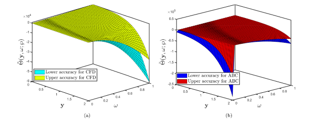
Fig. 11. Comparison of surface profile of Problem 5.3 established by considering (a) fuzzy CFD (b) fuzzy ABC fractional derivative operators when α=1 and uncertainty factor $\wp$∈[0,1]. |
From Fig. 12, (a and b) Comparison of multiple surface plots for different fractional orders with the fuzzy fractional CFD and ABC derivative operators are presented. Furthermore, it can be shown that by increasing the realistic representation of stream flow and groundwater dynamics on hillslopes in the plasma at $\wp$=.7.
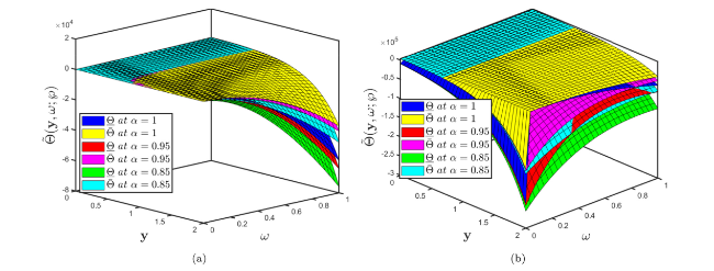
Fig. 12. Comparison of multiple surface profiles of Problem 5.3 established by considering (a) fuzzy CFD (b) fuzzy ABC fractional derivative operators when different fractional orders correlate with uncertainty factor $\wp$∈[0,1]. |
In Fig. 13 represents the comparison of the lower and upper accuracies between the fuzzy CFD and fuzzy ABC fractional derivative operators for different fractional orders when $\wp$∈[0,1] for expanding hydrologic descriptions at watershed scales.
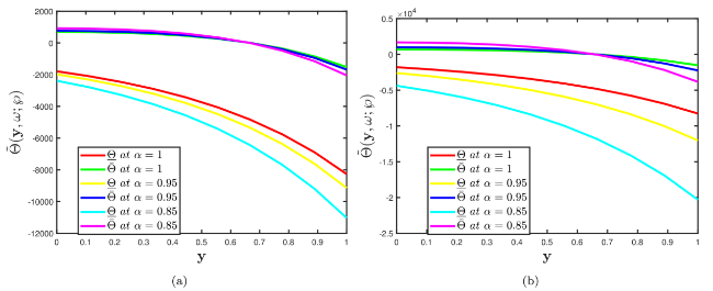
Fig. 13. Comparison of multiple two dimensional profiles of Problem 5.3 established by considering (a) fuzzy CFD (b) fuzzy ABC fractional derivative operators when different fractional orders correlate with uncertainty factor $\wp$∈[0,1]. |
In Fig. 14 shows the 2D comparison of the upper accuracies between the fuzzy CFD and fuzzy ABC fractional derivative operators when α=0.7. This creates a more conducive environment for analysing spatial relationships between ground topography and water table level.
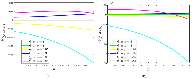
Fig. 14. Comparison of multiple two-dimensional profiles of the Problem 5.3 established by considering (a) fuzzy CFD (b) fuzzy ABC fractional derivative operators when fractional order α=0.7 correlate with the different uncertainty factors $\wp$∈[0,1]. |
In Fig. 15 gives the surface and 2D comparison by the fuzzy CFD and fuzzy ABC fractional derivative operators that show the interactions between the rainfall and runoff process.
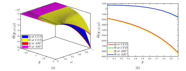
Fig. 15. Three dimensional comparison of Problem 5.3 established by considering (a) fuzzy CFD (b) fuzzy ABC fractional derivative operators when α=1 and uncertainty factor $\wp$∈[0,1]. |
The important element is that GIADM has provided pairs of solutions for the BSe, which is one of the most significant models in aquifers, with limited computational intricacy and concentration. When the constants in these solutions acquire a particular interpretation, they can be used to describe novel mechanisms of rainfall-runoff curves, irrigation and physical occurrences.
6. Conclusion
This novel family of solutions allows for the investigation and evolution of hydro-logical formulations with the aid of BSE correlated with the fuzzy set theory. Whereas other strategies are dependent on $\overline{\mathbf{y}}$ in some way, the solution described here is specifically reliant on the $\overline{\mathbf{y}}$ coordinate. This generates a highly supportive framework for evaluating complex features between elemental composition and water table elevation. Identifying the interaction between the generalized integral transform and the numerical method (ADM) assists us to comprehend how fuzzy fractional derivative operators work. The aforesaid transform applied here has the ability to generate several numerical solutions existing in the relative literature, see (Remark 2.1 and 3.1). Advanced methodology was utilized in the development of these findings. The merits and demerits of supplied strategies are examined. The findings elaborate on the similarities and differences between the two fuzzy fractional operators methodologies. The GIADM method is pragmatic for reducing computational costs. However, the GIADM has supremacy over the other numerical methods by avoiding the use of the Lagrange multiplier, stationary conditions, and intricate integrals are noise free. This is one of the advantages of the proposed scheme over the perturbation method. Also, considering that waves have a large impact on environmental issues along with beach side ocean and ocean engineering, the presented insights enable complete and practical research into the nature of these ripples, which may be used to develop meteorological pattern simulations.
7. Declarations
Availability of supporting data
No data were used to support this study.
Funding
Not Applicable.
Declaration of Competing Interest
The authors declare that they have no known competing financial interests or personal relationships that could have appeared to influence the work reported in this paper.
Acknowledgement
This work was supported by Taif University Researches Supporting Project number (TURSP- 2020/326), Taif University, Taif, Saudi Arabia.
