
1. Introduction
Differential equations (DEs) nonlinear phenomena are tremendously important in research (biology, physics, and chemistry). To account for physical phenomena, partial differential equations are utilized in mathematical modeling. Analytical, semi-analytical, and numerical approaches are employed to find solutions to PDEs because the nature of the solutions to PDEs affects the idea of physical phenomena. In the context of temporal and spatial derivatives, a novel class of nonlinear PDEs known as two-mode or dual-mode has just been described. Researchers have been exploring this problem and have discovered two-mode nonlinear PDEs, such as: two-mode(tm) mKdV [1], [2], tm KdV [3], [6], tm Sharma-Tasso-Olver [4], tm fifth order KdV [5], [7], two-mode Burger equation (tmBE) [8], tm perturbed Burger (tmPB) [9], tm KdV Burgers (tmKdVB) [10], tm Kadomtsev Petviashvili (tmKP) [11], [12], two-mode dispersive Fisher (tmdF) [13], tm Kuramoto-Sivashinsky (tmKS) [14], tm Boussinesq Burgers (tmBB) [15], two-mode coupled KdV (tmKdV) and mKdV (tm- CmKdV) [16], [17], two-mode non-linear Schrödinger (tmNLS) [18], and tm Hirota Satsuma coupled KdV(tmHSKdV) [19] equations and different analytical methodologies are used to create the dual-wave solutions. Among these techniques are: the -expansion method, the tanh expansion method, the Kudryshov method, the extended F-expansion method, therational sine-cosine method, the simplified Hirota's method, the sech-csch method, the tanh-coth method, the sinh-cosh method, the Fourier spectral technique, Exp-function method, Bcklund transformation scheme, Trigonometric function technique, the Bäcklund transformation based on the modified Kudryashov method, the modified Sardar sub-equation and q-homotopy analysis transform methods, the generalized auxiliary equation method, representation of the Kudryashov method, and the local meshless method [1], [2], [6], [7], [8], [9], [10], [11], [12], [13], [14], [15], [16], [17], [18], [19], [20], [21], [22], [23], [24], [25], [26], [27]. Some different models have been studied numerically and analytically by some researchers see [28], [29], [30], [31], [32]. Nonlinear phenomena in shallow water waves, stratified internal waves, and ion-acoustic waves in plasmas, can be presented using Korteweg-de Vries (KdV) equations. KdV-model equations can describe the positron-acoustic, ion-acoustic, electron-acoustic, magnetoacoustic, dust-acoustic, and quantum dust-ion-acoustic waves [33], [34]. The Sawada-Kotera equation is a KdV-type equations. In 2017, Wazwaz combine the sense of Korsunsky[35] and the framework of the SK equation, to offer the nonlinear dispersive equation, named as the two-mode SK equation(TfSK), given by:
where: is a field function presents the height of the water's free surface above a flat bottom, and are the nonlinearity and the dispersion parameters, respectively, , is related to the phase velocities and for , the two-mode TmSK is reduced to the SK equation after integrating with respect to . (1) interpret the propagation of two moving waves under the motivate of phase velocity , dispersion , and non-linearity factors. Wazwaz [5] apply the simplified Hirota method to derive multiple soliton solutions. Akbar et al. [36] studied the TmfKdV equation and attain some bright, kink, and singular periodic solutions via the Kudryashov and sine-cosine function methods. The authors in Kumar et al. [37] obtain bright, dark, periodic, and singular-periodic dual-wave solutions by the modified Kudryashov and new auxiliary equation methods. In [38] the improved F-expansion and generalized -expansion methods are used and numerous of solitary wave solutions of different kinds like bright and dark solitons, multi-peak soliton, breather type waves, periodic solutions. In this paper, we apply a new form of modified Kudryashov's method to attain analytical solutions of the Dual-mode Sawada Kotera equation. Our paper is organized as follows: In Section 1, we present an introduction, in the next section, we describe a modified Kudryashov's method presented for the first time. New soliton solutions are obtained in Section 3. In Section 4, the numerical solutions using the finite difference method are presented, the local truncation error for the difference scheme is disputed. Some graphs are investigated. Finally, the conclusion is presented in Section 5.
2. Portrayal of proposed method
2.1. The new form of modified Kudryashov's method
The general nonlinear equation can be written in the form:
where: is a polynomial of and the subscripts denotes the derivatives with respect to
Step 1: Using the following traveling wave transformation
where: is the wave number and is the speed of the wave. Implementation of the wave variable (3) in (2) yields an ordinary differential equation:
the prime indicates the derivative with respect to .
Step 2: Suppose that the solution of (4) can be expressed as a finite series in the form
where , are constants with to be calculated. is a positive integer will be determined using homogeneous balance principle.
Step 3: is defined as:
where: and are elective constants to be calculated. The function satisfy the following ODE:
the solution of (7) is given by
Step 4: By substituting (5) and using (6) and (8) in (4), we obtain a polynomial of . Putting all the terms of the like powers of equal to zero, we acquire a set of algebraic equations.
Step 5: Solving the system of algebraic equations using Mathematica software program to obtain a closed form of the exact solution.
3. Application of the method
Using the wave variable (3) then, Eq. (1) transformed to the ordinary differential equation as:
Eq. (9) was integrated twice, considering the constant of integration equal zero, we get
Balancing with , yields:
By the use of (5), we present the solution of (10) as:
Substituting (12) into (10), and collecting the terms of like powers of to zero, we acquire a set of algebraic equations:
Solving the previous system using the Mathematica program, we acquire four sets of solutions as follows: Set 1:
Substituting (13) in (12) with (6), (8) and (3), we get:
Set 2:
Substituting (15) in (12) with (6), (8) and (3), we obtain :
Set 3:
Substituting (17) in (12) with (6), (8) and (3), we acquire:
Set 4:
Substituting (19) in (12) with (6), (8) and (3), we get:
4. Finite difference method
We postulate as the exact solution and is the numerical solution both at the grid point . Substituting (21) into (1) we acquire the following set of difference equations:
The above system can be solved to obtain numerical values of .
4.1. Local truncation error
4.1.1. Lemma
The truncation error of the finite difference scheme (22) is of order:
Proof. To investigate the truncation error of the scheme (22), we anticipate Taylor's series expansion about the point when and , we get
Therefore,
□
4.2. The numerical results
In this part, some of the numerical results are presented for Dual mode Sawada Kotera equation. In Table 1 and Fig. 9 we discuss comparison between the numerical results and the analytical solution (14) for (1) at .
Table 1 Comparison between the numerical results with the analytical solution. |
| Numerical solution | Analytical solution | Absolute error | |
|---|---|---|---|
| 10.0 | 0.001191 | 0.001191 | 0.00000 |
| 8.0 | 0.006390 | 0.006390 | 2.82921 E 8 |
| 4.0 | 0.170018 | 0.170019 | 6.30489 E 7 |
| 0.0 | 1.046520 | 1.046510 | 2.14239 E 6 |
| 4.0 | 0.110301 | 0.110301 | 4.30451 E 7 |
| 8.0 | 0.004022 | 0.004022 | 1.77508 E 8 |
| 10.0 | 0.000749 | 0.000749 | 0.00000 |
In Table 2 and Fig. 10 we introduce comparison between the numerical results with the analytical solution (20) for (1) at .
Table 2 Comparison between the numerical results with the analytical solution . |
| Numerical solution | Analytical solution | Absolute error | |
|---|---|---|---|
| 10.0 | 0.535497 | 0.535497 | 0.00000 |
| 8.0 | 0.507140 | 0.507140 | 1.00230 E 7 |
| 4.0 | 0.145345 | 0.145345 | 3.49126 E 7 |
| 0.0 | 1.071890 | 1.071880 | 8.73319 E 6 |
| 4.0 | 0.053717 | 0.053718 | 4.76497 E 7 |
| 8.0 | 0.482552 | 0.482552 | 1.20561 E 7 |
| 10.0 | 0.527984 | 0.527984 | 0.00000 |
5. Graphical illustrations
Herein,we present some figures in the two-dimensional, three-dimensional to explain the presented solutions. Some of the analytical solutions are presented in Fig. 1, Fig. 2, Fig. 3, Fig. 4, Fig. 5, Fig. 6, Fig. 7, Fig. 8. In Fig. 1, we introduce the graph of (14) at . In Fig. 2, the solution of (14) is plotted when some parameters are changed. Also, the graph of (16) at , is presented in Fig. 3. In Fig. 4, the solution of (16) is plotted when some parameters are changed. Moreover, we introduce the graph of (18) at in Fig. 5. In Fig. 6, we introduce the solution of (18) when some parameters are varied. The graph of (20) at is given in Figs. 7 and 8, the solution of (20) is plotted when some parameters are changed. At the end, the differences between the analytical solutions and numerical solutions are presented by graphs in Figs. 9 and 10 at .
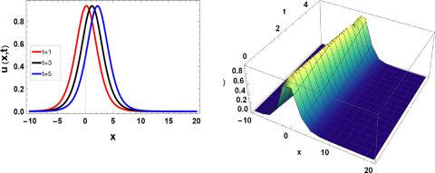
Fig.1 Graph of (14) at . |
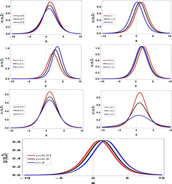
Fig.2 Graph of (14) when some parameters are changed. |
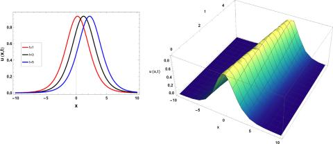
Fig.3 Graph of (16) at . |
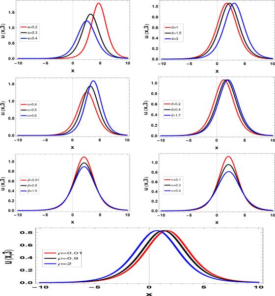
Fig.4 Graph of (16) when some parameters are changed. |
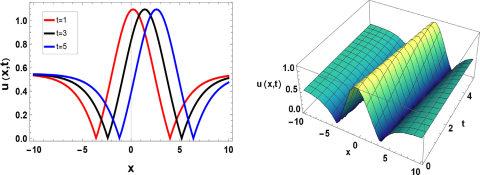
Fig.5 Graph of (18) at . |
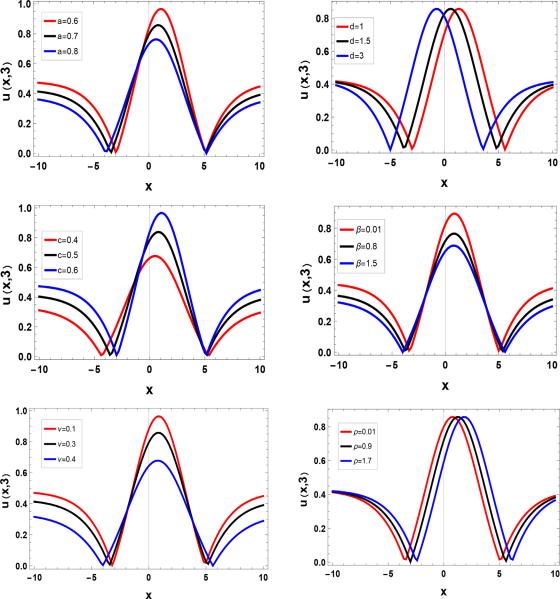
Fig.6 Graph of (18) when some parameters are changed. |
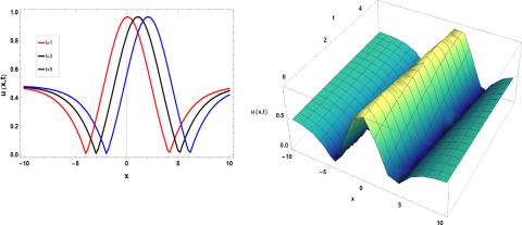
Fig.7 Graph of (20) at . |
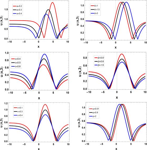
Fig.8 Graph of (20) when some parameters are changed. |
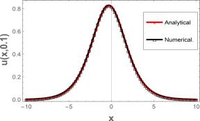
Fig.9 Rapprochement between the numerical solution of (1) and the analytical solution (14) at . |
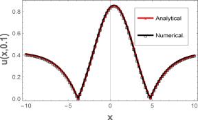
Fig.10 Rapprochement between the numerical solution of (1) and the analytical solution (20) at . |
6. Discussion
For describing solutions, a graph is a useful tool. For the specified values of the parameters, the 2D and 3D profile of (14) is a bell shape soliton, as illustrated in Fig. 1, showing that the wave travels to the right with increasing time. Fig. 2 describes the behavior of traveling waves with different parameters for (14). The increment in cause decrease in the amplitude and the wave travels to the left, also it advances to the right when and increase, moreover, an increase in amplitude arise when increases and the wave transfer towards right, in addition, the amplitude of wave decreases with and increase, finally, the wave travels towards left when increases.
The 2D and 3D profile of (16) is a bell shape soliton, as illustrated in Fig. 3, we notice the transfer of the wave to the right with increasing time. In Fig. 4 We can detect a decrease in amplitude and the wave is moving to the left as increases, also it advances to the right when and increase, moreover the wave moves to the right and the amplitude increases with increases, in addition, the amplitude of wave decreases with and increase, finally, the wave transfer to the left with increases.
As shown in Fig. 5, the 2D and 3D profile of (18) is a bell shape soliton with a tail in the wave, indicating that the wave advances to the right with increasing time. In Fig. 6 as increases the wave travels towards left and the amplitude is reduced, it also advances to the left as increases, when increases the wave is moving towards right and there is a rise in amplitude, the amplitude of the wave decreases as and increase, and the wave finally is moving to the right as increases.
The 2D and 3D profile of (20) is a bell shape soliton with a tail in the wave, as illustrated in Fig. 7, illustrating that the wave advances to the right with increasing time. In Fig. 8 we can see the leftward advance of the wave and the amplitude decreases with increases, also it advances to the right when increases, moreover with an increase in , the wave advances to the right and The amplitude grows, in addition, the amplitude of wave decreases with and increase, finally, the wave travels to the left with increases.
The 2D profiles of Figs. 9 and 10 describe the rapprochement between our numerical results of (1) and the analytical solution (14) and the analytical solution (20) respectively.
7. Conclusion
Finally, we presented a new form of modified Kudryashov's method (NMK) to study the Dual-mode Sawada Kotera model. From the premise that we want to improve solutions and explain physical phenomena optimally, we developed the modified Kudryashov method and put it in a general form that contains more than one controllable constant. We have studied the model in this way and presented figures showing the correctness of what we hoped to reach from the proposed method. In addition, we presented an extensive numerical study of this model using the finite differences method. We also came up with the local truncation error for the difference scheme is . In addition, the analytical solutions and the numerical solutions were compared. Through what we have reached, we can say that our results are a clear contribution in this field. At the end of our article, we present a future plan for our study, as we can solve more than one model in this way, and we can also develop other ways to solve different models.
Declaration of Competing Interest
Authors declare that they have no conflict of interest.
