
1. Introduction
Diffusion is a natural phenomenon that occurs in chemical, physical, and biological models. In general, diffusive processes are commonly used to understand the effect of particles spread in different systems. For instance, in homogeneous medium governed by the classical Brownian motion [1].
where is the probability distribution function at position and time , is the constant flow speed, with the spatial diffusion coefficient.
Recently, different studies of biological, physical and astrophysical systems have showed that the diffusion of particles is often exhibited anomalous behavior [3], [4], [5]. Anomalous transport (non-diffusive motion) can be classified based on the mean square displacement of particle grows as , with and corresponding to subdiffusion and superdiffusion respectively. The super-diffusive is suggested for the transport of energetic particles [6], [7], molecular transport in living cells [8], and in diffusion of liquid-solid interface [9]. Sub-diffusive was observed in amorphous semiconductors [3], neutron transport [10], transport of energetic particles in solar wind [11], and proton transport in perfluorosulfonic acid membranes [12].
A number of theoretical studies have explored anomalous diffusion using frameworks of continuous time random walks [13], [14]. For instance, fractional kinetic equations, in which space or time-fractional derivatives or both are exist [15], [16]. Fractional differential equations with time or space fractional derivatives are widely used to describe various complex phenomena in many fields such as meteorological forecasts [17], Lakes pollution [18], astrophysics [19], [20], electronic circuits [21], plasma physics [22] and in others discipline field of science. In general, the space-fractional diffusion model still describes a non-Markov process, while the diffusion equations with a time fractional derivative describes a non-Markovian process and can lead to subdiffusion and superdiffusion [23], [24].
According to that, the classical diffusion equation can be generalized by replaced the time derivatives with a fractional derivatives. This generalization is recover different situation of the non-diffusive transport mechanism according to the mean square displacement behavior. However, there are different fractional derivative with different physical interpolation. The definitions of fractional derivative divided into the singular derivatives [25], and non-singular fractional derivative [26]. Our main focus here is on the Caputo fractional derivative [27], which provides initial conditions with a physical interpretation [28].
On the other hand, Evans and Majumdar [29] have proposed a diffusion model with stochastic resetting to study the intermittency of a particle's search process. Further, the mathematical analysis of diffusion under resetting is developed to study the comb-like structures [30], [31], holographic optical tweezers [32] and quantum dynamics [33]. Moreover, this studies are extended to the general models of kinetic problems such as telegraphic process [34], fractional kinetics equation [35], [36], and a random walk with Lévy flight [37]. From here and for the first time we extended the theory of stochastic resetting to the fractional diffusion-advection equation [7]. We search for a general solution of the fractional resetting model, which can be obtained based on re-scaling of the waiting times and jumps in the manner used in [37].
In this paper, the fractional diffusion-advection equation under resetting assumption is considered in Section 2. And by using the Laplace and Fourier transforms, we obtain a general analytical solution of the fractional resetting model. In Sections 3 and 4, as an illustration we present the fractional-order and resetting rate effects on the behavior of probability distribution functions with the different classes of mean square displacement behavior. Finally, the summary of our findings closes out the paper.
2. Analytical solution of the fractional diffusion-advection equation under resetting assumption
In this section, we consider a particle stochastically resets to a position at with a constant rate . And instead of a time-derivative, which lead to Gaussian diffusion, we insert a non-local fractional derivative characteristic of waiting time in sense of Caputo's fractionald derivative. In such case the PDF satisfies the fractional form of Eq. (1), which is given by
with initial condition . Equation (2) is analogous to the diffusion-advection equation defining a model of diffusion with stochastic resetting.
Let us search for solution by using Laplace-Fourier technique. Therefore, Eq. (2) in Laplace domain is given by
And in Fourier space, we obtain
Then, Eq. (2) in Laplace-Fourier domains is given by
For simplicity, we can say
where
and
The inverse Laplace-Fourier transforms of can be calculated trough calculate the inverse of Eqs. (8) and (9). We start by calculate the inverse Laplace and Fourier transforms of and by following the same procedures, one can obtain the inverse transforms of
First, we consider
and,
Where,
and,
First, we calculate the inverse-Fourier transform of Eq. (12) as follows:
Thus,
Second, we calculate the inverse-Laplace transform of as follow:
which be expressed as
Via the property used in [41], the function is given by
where, is the M-Wright function defined as [41]
From Eqs. (16) and (19), is given by
By following the same manner, the function is expressed as follow
Thus,
where is the Foxs H function [42].
From Eqs. (16) and (23), we find
Directly from Eqs. (21) and (24), the solution of the fractional diffusion-advection equation including resetting assumption is
We can test our general solution Eq. (25) by set , thus we obtain
which represent a general solution of the time-fractional diffusion-advection equation and is reduced to the solution of the classical diffusion-advection equation in the case of as follows:
Furthermore, from Eq. (25), we show that in the absence of resetting , we do not have a stationary state. However, the solution with nonzero resetting leads to a stationary state. In an analogue way, one can obtain the stationary density in diffusive case under resetting assumption from Eq. (25) at , which is given by
In case of (without advection term), the above integral is reduced to the familiar stationary distribution under stochastic resetting [29], which is give by
The PDF Eq. (29) is evidently non-Gaussian with a cusp making a non-equilibrium stationary.
3. Mean square displacement analysis
Now, one can calculate the mean square displacement (MSD) of a particle via the following identity [15]:
by imposing Eq. (6) into Eq. (30), one obtains
where . Then, Eq. (31) can be expressed as:
According to that, the MSD of the time-fractional diffusion-advection equation under resetting is equal
where,
and,
For long time , one obtains
And for short times , the MSD Eq. (33) is equal
Besides that, from Eq. (37), one can get the MSD of particle density without resetting ( ), which is given by
Also, in case of , we obtain the MSD for the diffusion-advection equation with resetting in the form
which corresponds to MSD of non-fractional diffusion-advection equation with resetting on a comb-like structure, see [30]. At and with neglecting the advection term , the MSD Eq. (39) is reduced to the MSD of the diffusion equation with exponential diffusivity (the so-called Dodson diffusion equation)
which at long times, it rapidly tends to steady-state
Also, one can obtains the MSD for the typical case of sub-diffusion [15], by setting and in Eq. (39), which is given by
which leads to the standard Brownian motion at as follow:
4. Discussion
In this article, we have solved the fractional diffusion-advection equation, which is superior to the previous fractional models treating non-diffusive transport models because it includes the resetting assumption. Here, shed light on the comparison between the diffusion and diffusion-advection models for different values of time fractional-orders and resetting rates with the typical behavior of the MSD in different cases.
In Fig 1, the diffusive models is illustrated for the diffusion case with different values of time fractional order , but with zero resetting rate (left panel), while the right panel of Fig 1 illustrate the PDFs for different values of resetting rate in non-fractional case . Further, the diffusion-advection solution Eq. (25) is illustrated also for different fractional order with zero resetting (right panel), and for different resetting values in non-fractional case (left panel). From Figs. 1 and 2, one can show that, the cusp-shapes of the PDFs do not appear only for the change of the time fractional-order, but appearing also in the case of change of resetting rate values. In addition to that, Fig. 2 presented the asymmetric density profile associated to the contribution of the advection term in both cases. And in case of the fractional diffusion-advection (left panel Fig. 1, Fig. 2) the sudden sharp variations occur and they become less sharp in case of the advection-diffusion with resetting (Right panel Fig. 1, Fig. 2). According to that, many prediction of the evolution of the PDFs can be determine based on the change of fractional order and resetting rate values.

Fig.1 PDF Eq. (25) in case of (without advection term). |
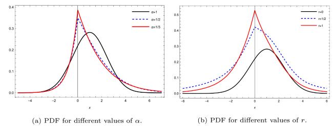
Fig.2 PDF Eq. (25) in case of (with advection term). |
Moreover, From Eq. (33), one can find the typical behavior of the MSD for different values of fractional order and resetting rate . Fig. 3, Fig. 4, Fig. 5, Fig. 6 exhibits sub-diffusion due to the power-law dependence of MSD on time. This is in contrast to a normal diffusion process where a particle's MSD follows a linear with time. Furthermore, the obtained results illustrated in Fig. 3, Fig. 4, Fig. 5, Fig. 6 for the fractional advection-diffusion equation in both resetting and non-resetting assumptions are in agreement with [14], [15], [30]. In addition to that, from the left panel of Fig. 3, Fig. 4, one can show that, the resetting rate can changes the character of long time solution. And from Fig. 3, Fig. 4, Fig. 5, Fig. 6, we can show increasing the value of resetting rate leads to the steady state behavior.
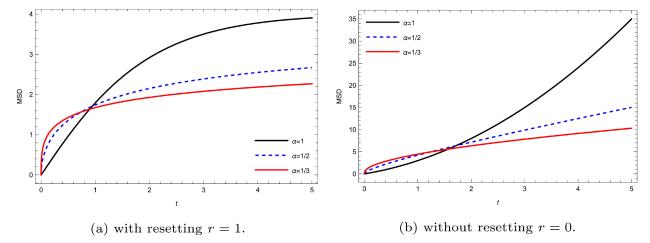
Fig.3 MSD for different values of in case of . |
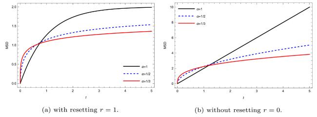
Fig.4 MSD for different values of in case of . |
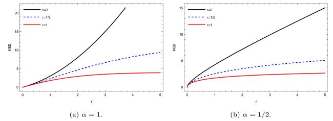
Fig.5 MSD for different values of resetting rate in case of . |
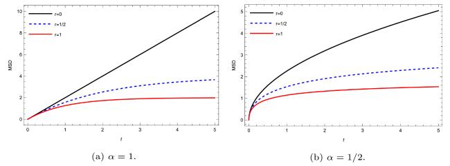
Fig.6 MSD for different values of resetting rate in case of . |
From the above results, we find that, the solution of the fractional advection-diffusion equation under resetting given by Eq. (25) is a general analytical solution describing the non-diffusive theory of particles transport. Moreover, the fractional model presented here recovers many approximations describe anomalous transport, such as fractional diffusion model [16], [41] and classical diffusion equation with resetting [4], [29], which are describe the PDFs in many physical and biological models [4].
In summary, we have considered in this article the time-fractional resetting diffusion-advection equation using Caputo's fractional operator. To solve the fractional equation, we used a joint Laplace-Fourier transform. The solution is given in terms of M-Wright and Foxs H functions.Our new solution has been illustrated as related to anomalous behaviours with more accurate results for various kinds of MSD based on the values of the time-fractional order and resetting rate.
Declaration of Competing Interest
The authors declare that they have no known competing financial interests or personal relationships that could have appeared to influence the work reported in this paper.
