An extensive analytical and numerical study of the generalized q -deformed Sinh-Gordon equation

Khalid K. Ali; Abdel-Haleem Abdel-Aty

doi:10.1016/j.joes.2022.05.034

Journal of Ocean Engineering and Science >

2024 , Vol. 9 >Issue 3: 232 - 239

DOI: https://doi.org/10.1016/j.joes.2022.05.034

Original article

An extensive analytical and numerical study of the generalized q -deformed Sinh-Gordon equation

Khalid K. Ali ^,^a^,^* ,
Abdel-Haleem Abdel-Aty ^,^b^,^c

Expand

^a Mathematics Department, Faculty of Science, Al-Azhar University, Nasr-City, Cairo, Egypt
^b Department of Physics, College of Sciences, University of Bisha, PO Box 344, Bisha 61922, Saudi Arabia
^c Physics Department, Faculty of Science, Al-Azhar University, Assiut 71524, Egypt

^*E-mail addresses: khalidkaram2012@azhar.edu.eg (K.K. Ali);

amabdelaty@ub.edu.sa (A.-H. Abdel-Aty).

Received date: 2022-04-29

Revised date: 2022-05-22

Accepted date: 2022-05-29

Online published: 2022-06-01

Fold

Abstract

In this paper, the q-deformed Sinh-Gordon equation is solved analytically using a new general form based on the extended tanh approach. The numerical solutions of the equation is obtained using a b-spline finite element method. Also, we present numerous figures to demonstrate the various solitons propagation patterns. This type of equation has not been previously dealt with in such ways, whether analytical or numerical. This study is very useful in studying several physical systems that have lost their symmetry.

Highlights

● The q-deformed Sinh-Gordon equation was investigated analytically using the new general form of the extended tanh approach and numerically using a b-spline finite element method in this paper.

● We also present numerous figures to demonstrate the various solitons propagation patterns.

● This type of equation has not been previously dealt with in such ways, whether analytical or numerical.

● We believe that this study will be very useful in studying physical systems that have lost their symmetry.

Key words： q -Deformed equation; Solitos solutions; The extended tanh method; Finite element method; q-Calculus

Cite this article

Khalid K. Ali , Abdel-Haleem Abdel-Aty . An extensive analytical and numerical study of the generalized q -deformed Sinh-Gordon equation[J]. Journal of Ocean Engineering and Science, 2024 , 9(3) : 232 -239 . DOI: 10.1016/j.joes.2022.05.034

1. Introduction

Nonlinear systems attracted much interest due to it's importance in explaining the dynamics of many systems in natures and science such as, gravitational waves, acoustics plasma waves, shallow water dynamics, no-linear optics, fluid dynamics and surface ocean waves [1], [2], [3], [4], [5], [6]. The microscopic systems that are governed by the principles of quantum physics is considered as a best example of q-deformed Sinh-Gordon equation [7], [8]. Many mathematical models describing some physical systems have been extensively studied by a group of researchers [9], [10], [11], [12], [13], [14], [15], [16], [17], [18], [19], [20], [21], [22], [23], [24].

Quantum calculus, often known as calculus without bounds, is the same as regular infinitesimal calculus but without the concept of bounds. It defines ”

q

-calculus” and ”

h

-calculus”, where

h

ostensibly stands for Planck's constant while

q

stands for quantum. The two parameters are related by the formula [25]

(1.1)

q = e^{i h} = e^{2 i π ℏ},

where

ℏ = \frac{h}{2 π}

. The study of the equations containing

q

-calculus has not been covered except in limited papers such as [26], [27].

q

-calculus, this area of research has several applications there are several developments and applications of the

q

-calculus in mathematical physics, the theory of relativity and special functions [28], [29], [30], [31], [32], [33].

The study of the generalized

q

-deformed Sinh-Gordon equation (Eleuch equation) is the subject of this article [26], [27]. Eleuch equation is written as:

(1.2)

\frac{\partial^{2} Ω}{\partial x^{2}} - \frac{\partial^{2} Ω}{\partial t^{2}} = {[\sinh_{q} (β Ω^{α})]}^{m} - ϑ .

where

α, m

are constantes and

q \in (0, 1)

. For

q = 1

gives the standard Sinh-Gordon equation.

In this work, we use the extended tanh approach to examine the soliton solutions of (1.2) [34], [35]. Besides, we solve this equation numerically using the b-spline finite element method [36], [37], [38], [39]. We study two cases for this equation.

This paper has been organized as follows: The second section presents some definitions and properties of

q

-calculus. In the third section, we present the methodology of the analytical method. In the fourth section, we present the solutions obtained. In the fifth section, we present the numerical solutions to the equation. In the sixth section, we present some different forms of solutions. In the seventh section, we present a conclusion of what we have done in the work.

2. q-Calculus

Now, we introduce some basic definitions of the

q

-calculus as follows: [33]

● For any real number

a

, let us define

{[a]}_{q}

{[a]}_{q} = \frac{1 - q^{a}}{1 - q}, a \in R .

● In the

q

-calculus, differential of function is defined as:

d_{q} (f (t)) = f (q t) - f (t) .

● The

q

-gamma function is defined by

Γ_{q} (t) = \frac{G (q^{t})}{{(1 - q)}^{t - 1} G (q)}, t \in R - {0, - 1, - 2, \dots},

where

G (q^{t}) = \frac{1}{{(q^{t}; q)}_{\infty}} .

Or, equivalently,

Γ_{q} (t) = \frac{1 - q^{(t - 1)}}{1 - q^{t - 1}},

and satisfies

Γ_{q} {(t) + 1) = [t]}_{q} Γ_{q} (t) .

● The

q

-derivative of a function

f

is given by

(D_{q} f) (t) = \frac{d_{q} (f (t))}{d_{q} (t)} = \frac{f (t) - f (t q)}{t - q t}, (D_{q} f) (0) = \lim_{t \to \infty} (D_{q} f) (t) .

● The

\sinh_{q}

is defined by:

\sinh_{q} (t) = \frac{e^{t} - q e^{- t}}{2},

● The

\cosh_{q}

is defined by:

\cosh_{q} (t) = \frac{e^{t} + q e^{- t}}{2},

● We list below some simple and useful relations for

q

-deformed functions

{(\cosh_{q} (t))}^{2} - {(\sinh_{q} (t))}^{2} = q,

\sinh_{q} - t) = - q \sinh_{\frac{1}{q}} (t),

\cosh_{q} - t) = q \cosh_{\frac{1}{q}} (t),

\frac{d}{d t} \cosh_{q} (t) = \sinh_{q} (t),

\begin{matrix} \frac{d}{d t} \sinh_{q} (t) = \cosh_{q} (t), \\ ⋮ \end{matrix}

3. Mathematical analysis of the model

The following transformation is used to determine the traveling wave solution of (1.2),

(3.1)

Ω (x, t) = u (δ),

where

(3.2)

δ = a x - c t + θ .

where

c

denotes the speed of traveling wave. Using (3.1) and (3.2), then (1.2) becomes,

(3.3)

(a^{2} - c^{2}) u^{″} (δ) + ϑ - [{sinh}_{q} u {(δ)}^{α})]^{m} = 0 .

Now, we take two cases for (3.3).

● Case one: Suppose

m = α = 1, ϑ = 0 .

Then, (3.3) can be written as:

(3.4)

(a^{2} - c^{2}) u^{″} (δ) - {sinh}_{q} (u (δ)) = 0 .

We can multiply both side of (3.4) by

u^{'} (δ)

and after the integration we get

(3.5)

\frac{1}{2} (a^{2} - c^{2}) {(u^{'} (δ))}^{2} - {cosh}_{q} (u (δ)) - c_{1} = 0,

where

c_{1}

is a constant of the integration.

Let

(3.6)

u (δ) = l n (v (δ)) .

Thus, (3.5) becomes,

(3.7)

(c^{2} - a^{2}) v^{' 2} (δ) + 2 C_{1} v^{2} (δ) + q v (δ) + v^{3} (δ) = 0 .

Thus, we can solve (3.7) using our method and from (3.6) and (3.1) we can get the solution of (1.2) in the first case.

● Case two: Suppose

α = 1, m = 2, ϑ = - \frac{q}{2} .

Then, (3.3) can be written as:

(3.8)

(a^{2} - c^{2}) u^{″} (δ) - {({sinh}_{q} (u (δ)))}^{2} + \frac{q}{2} = 0 .

After simplify (3.8) we get

(3.9)

(a^{2} - c^{2}) u^{″} (δ) - \frac{1}{2} {cosh}_{q}^{2} (2 u (δ)) = 0 .

Let

(3.10)

u (δ) = \frac{1}{2} l n (v (δ)) .

Thus, (3.10) becomes,

(3.11)

2 (a^{2} - c^{2}) v^{' 2} (δ) - 2 (a^{2} - c^{2}) v (δ) v^{″} (δ) + q^{2} v (δ) + v^{3} (δ) = 0 .

Thus, we can solve (3.11) using our method and from (3.10) and (3.1) we can get the solution of (1.2) in the second case.

4. The strategy of the extended tanh function method

Postulate the governing equation in the form

(4.1)

F (Ω, Ω_{x x}, Ω_{t t}, \dots) = 0,

where:

F

is a polynomial

Ω = Ω (x, t)

and its partial derivatives. Applying a traveling wave transformations to convert (3.1) to an ordinary differential equation:

(4.2)

H (u, u^{″}, \dots) = 0 .

The essential steps of the new generalization for the Extended

\tanh

function method are:

Step 1: The modified extended tanh method present the solution of (4.2) by the following finite series:

(4.3)

u (δ) = A_{0} + \sum_{i = 1}^{N} (A_{i} ϕ {(δ)}^{i} + B_{i} ϕ {(δ)}^{- i}),

where

ϕ = ϕ (δ)

, satisfy the Riccati equation

(4.4)

\frac{d ϕ}{d δ} = ϱ + ϕ^{2} .

The solution of the Riccati Eq. (4.4) has the following cases of solutions: If

ϱ < 0

then

(4.5)

\begin{matrix} ϕ (δ) = - \sqrt{- ϱ} \tanh (\sqrt{- ϱ} δ), \\ ϕ (δ) = - \sqrt{- ϱ} \coth (\sqrt{- ϱ} δ) . \end{matrix}

ϱ = 0

then

(4.6)

ϕ (δ) = - \frac{1}{δ} .

ϱ > 0

then

(4.7)

\begin{matrix} ϕ (δ) = \sqrt{ϱ} \tan (\sqrt{ϱ} δ), \\ ϕ (δ) = - \sqrt{ϱ} \cot (\sqrt{ϱ} δ) . \end{matrix}

Step 2:

N

can be determined by balancing the highest order derivative term with the highest power nonlinear term in (4.2).

Step 3: Substituting (4.3) and (4.4) into (4.2) then gather all coefficients of the same powers of

ϕ {(δ)}^{i}

and put them equal to zero, we get a system of algebraic equations for

ϱ, A_{0}, \dots, A_{N}, B_{1}, \dots, B_{N}

, solving this equations we get all constants.

5. The analytical solution for the model

In this section, the generalization of kudryashov method applies to find the analytic solution to the two cases that were imposed for the Eq. (1.2)

● The analytical solution of case one at

m = α = 1, ϑ = 0

Applying the balance principle in (3.7) between

v^{' 2}

and

v^{3}

we get

2 N + 2 = 3 N \Rightarrow N = 2

. From (4.3), the solution of (3.7) can be presented as:

(5.1)

v (δ) = A_{0} + \sum_{i = 1}^{2} (A_{i} ϕ {(δ)}^{i} + B_{i} ϕ {(δ)}^{- i}) .

Substituting (5.1) into (3.7), setting the coefficient of like power of

ϕ (δ)

equal to zero, we acquire the following system:

4 a^{2} A_{1} B_{1} ϱ + 16 a^{2} A_{2} B_{2} ϱ - a^{2} A_{1}^{2} ϱ^{2} - a^{2} B_{1}^{2} - 4 A_{1} B_{1} c^{2} ϱ - 16 A_{2} B_{2} c^{2} ϱ

+ 4 A_{1} B_{1} c_{1} + 4 A_{2} B_{2} c_{1} + 6 A_{1} A_{0} B_{1} + 6 A_{2} A_{0} B_{2} + 3 A_{2} B_{1}^{2} + 3 A_{1}^{2} B_{2} + A_{1}^{2} c^{2} ϱ^{2}

+ 2 A_{0}^{2} c_{1} + A_{0} q + A_{0}^{3} + B_{1}^{2} c^{2} = 0,

8 a^{2} A_{2} B_{1} ϱ + 4 a^{2} A_{1} B_{2} - 4 a^{2} A_{1} A_{2} ϱ^{2} - 8 A_{2} B_{1} c^{2} ϱ - 4 A_{1} B_{2} c^{2}

+ 4 A_{2} B_{1} c_{1} + 3 A_{1}^{2} B_{1} + 6 A_{0} A_{2} B_{1} + 6 A_{1} A_{2} B_{2} + 4 A_{1} A_{2} c^{2} ϱ^{2} + 4 A_{0} A_{1} c_{1}

+ A_{1} + q + 3 A_{0}^{2} A_{1} = 0,

2 a^{2} A_{1} B_{1} + 8 a^{2} A_{2} B_{2} - 4 a^{2} A_{2}^{2} ϱ^{2} - 2 a^{2} A_{1}^{2} ϱ - 2 A_{1} B_{1} c^{2} - 8 A_{2} B_{2} c^{2}

+ 6 A_{1} A_{2} B_{1} + 3 A_{2}^{2} B_{2} + 4 A_{2}^{2} c^{2} ϱ^{2} + 2 A_{1}^{2} c^{2} ϱ + 2 A_{1}^{2} c_{1}

+ 4 A_{0} A_{2} c_{1} + A_{2} q + 3 A_{0} A_{1}^{2} + 3 A_{0}^{2} A_{2} = 0,

4 a^{2} A_{2} B_{1} - 8 a^{2} A_{1} A_{2} ϱ - 4 A_{2} B_{1} c^{2} + 3 A_{2}^{2} B_{1} + 8 A_{1} A_{2} c^{2} ϱ

+ 4 A_{1} A_{2} c_{1} + A_{1}^{3} + 6 A_{0} A_{1} A_{2} = 0,

- 4 a^{2} A_{1} A_{2} + 4 A_{1} A_{2} c^{2} + 3 A_{1} A_{2}^{2} = 0,

- 8 a^{2} A_{2}^{2} ϱ - a^{2} A_{1}^{2} + 8 A_{2}^{2} c^{2} ϱ + A_{1}^{2} c^{2} + 2 A_{2}^{2} c_{1} + + 3 A_{2} A_{1}^{2} + 3 A_{0} A_{2}^{2} = 0,

- 4 a^{2} A_{2}^{2} + 4 A_{2}^{2} c^{2} + A_{2}^{3} = 0,

4 a^{2} A_{2} B_{1} ϱ^{2} + 8 a^{2} A_{1} B_{2} ϱ - 4 a^{2} B_{1} B_{2} - 4 A_{2} B_{1} c^{2} ϱ^{2} - 8 A_{1} B_{2} c^{2} ϱ

+ 4 A_{0} B_{1} c_{1} + 4 A_{1} B_{2} c_{1} + 3 A_{1} B_{1}^{2} + 3 A_{0}^{2} B_{1} + 6 A_{0} A_{1} B_{2} + 6 A_{2} B_{1} B_{2}

+ 4 B_{1} B_{2} c^{2} + B_{1} + q = 0,

+ 2 a^{2} A_{1} B_{1} ϱ^{2} + 8 a^{2} A_{2} B_{2} ϱ^{2} - 2 a^{2} B_{1}^{2} ϱ - 4 a^{2} B_{2}^{2} - 2 A_{1} B_{1} c^{2} ϱ^{2}

- 8 A_{2} B_{2} c^{2} ϱ^{2} + 4 A_{0} B_{2} c_{1} + 3 A_{0} B_{1}^{2} + 3 A_{2} B_{2}^{2} + 3 A_{0}^{2} B_{2}

+ 6 A_{1} B_{1} B_{2} + 2 B_{1}^{2} c^{2} ϱ + 4 B_{2}^{2} c^{2} + 2 B_{1}^{2} c_{1} + B_{2} q = 0,

- a^{2} B_{1}^{2} ϱ^{2} - 8 a^{2} B_{2}^{2} ϱ + 3 A_{0} B_{2}^{2} + B_{1}^{2} c^{2} ϱ^{2} + 8 B_{2}^{2} c^{2} ϱ + 2 B_{2}^{2} c_{1} + 3 B_{2} B_{1}^{2} = 0,

4 a^{2} A_{1} B_{2} ϱ^{2} - 8 a^{2} B_{1} B_{2} ϱ - 4 A_{1} B_{2} c^{2} ϱ^{2}

+ 3 A_{1} B_{2}^{2} + 6 A_{0} B_{1} B_{2} + 8 B_{1} B_{2} c^{2} ϱ + 4 B_{1} B_{2} c_{1} + B_{1}^{3} = 0,

- 4 a^{2} B_{1} B_{2} ϱ^{2} + 4 B_{1} B_{2} c^{2} ϱ^{2} + 3 B_{1} B_{2}^{2} = 0,

- 4 a^{2} B_{2}^{2} ϱ^{2} + 4 B_{2}^{2} c^{2} ϱ^{2} + B_{2}^{3} = 0 .

Solving the previous set of equations with the aid of Mathematica program, we obtain the following set of solutions.

● Class 1:

(5.2)

\begin{matrix} A_{0} = \frac{\sqrt{q}}{2}, A_{1} = 0, A_{2} = - \frac{\sqrt{q}}{4 ϱ}, B_{1} = 0, \\ B_{2} = - \frac{\sqrt{q} ϱ}{4}, a = \mp \sqrt{c^{2} - \frac{\sqrt{q}}{16 ϱ}}, c_{1} = - \sqrt{q} . \end{matrix}

Substituting from (5.2) into (5.1) with (4.5), (4.6), (4.7), (3.6) and (3.1), we get the solutions of (1.2) at

m = α = 1, ϑ = 0

ϱ < 0

, then

(5.3)

\begin{matrix} Ω_{1, 2} (x, t) & = l n (A_{2} {(- \sqrt{- ϱ} \coth ((a x - c t + θ) \sqrt{- ϱ}))}^{2} + A_{0} \\ + \frac{B_{2}}{{(- \sqrt{- ϱ} \coth ((a x - c t + θ) \sqrt{- ϱ}))}^{2}}) . \end{matrix}

(5.4)

\begin{matrix} Ω_{3, 4} (x, t) & = l n (A_{2} {(- \sqrt{- ϱ} \tanh ((a x - c t + θ) \sqrt{- ϱ}))}^{2} + A_{0} \\ + \frac{B_{2}}{{(- \sqrt{- ϱ} \tanh ((a x - c t + θ) \sqrt{- ϱ}))}^{2}}) . \end{matrix}

ϱ > 0

, then

(5.5)

\begin{matrix} Ω_{5, 6} (x, t) & = l n (A_{2} {(- \sqrt{ϱ} \cot ((a x - c t + θ) \sqrt{ϱ}))}^{2} + A_{0} \\ + \frac{B_{2}}{{(- \sqrt{ϱ} \cot ((a x - c t + θ) \sqrt{ϱ}))}^{2}}) . \end{matrix}

(5.6)

\begin{matrix} Ω_{7, 8} (x, t) & = l n (A_{2} {(\sqrt{ϱ} \tan ((a x - c t + θ) \sqrt{ϱ}))}^{2} + A_{0} \\ + \frac{B_{2}}{{(\sqrt{ϱ} \tan ((a x - c t + θ) \sqrt{ϱ}))}^{2}}) . \end{matrix}

● Class 2:

(5.7)

\begin{matrix} A_{0} = 0, A_{1} = 0, A_{2} = - \frac{\sqrt{q}}{ϱ}, B_{1} = 0, \\ B_{2} = 0, a = \mp \sqrt{c^{2} - \frac{\sqrt{q}}{4 ϱ}}, c_{1} = - \sqrt{q} . \end{matrix}

Substituting from (5.7) into (5.1) with (4.5), (4.6), (4.7), (3.6) and (3.1), we get the solutions of (1.2) at

m = α = 1, ϑ = 0

ϱ < 0

, then

(5.8)

\begin{matrix} Ω_{9, 10} (x, t) & = l n (A_{2} {(- \sqrt{- ϱ} \coth ((a x - c t + θ) \sqrt{- ϱ}))}^{2}) . \end{matrix}

(5.9)

\begin{matrix} Ω_{11, 12} (x, t) & = l n (A_{2} {(- \sqrt{- ϱ} \tanh ((a x - c t + θ) \sqrt{- ϱ}))}^{2}) . \end{matrix}

ϱ > 0

, then

(5.10)

\begin{matrix} Ω_{13, 14} (x, t) & = l n (A_{2} {(- \sqrt{ϱ} \cot ((a x - c t + θ) \sqrt{ϱ}))}^{2}) . \end{matrix}

(5.11)

\begin{matrix} Ω_{15, 16} (x, t) & = l n (A_{2} {(\sqrt{ϱ} \tan ((a x - c t + θ) \sqrt{ϱ}))}^{2}) . \end{matrix}

● Class 3:

(5.12)

\begin{matrix} A_{0} = 0, A_{1} = 0, A_{2} = 0, B_{1} = 0, B_{2} = \sqrt{q} ϱ, \\ a = \mp \sqrt{c^{2} + \frac{\sqrt{q}}{4 ϱ}}, c_{1} = \sqrt{q} . \end{matrix}

Substituting from (5.12) into (5.1) with (4.5), (4.6), (4.7), (3.6) and (3.1), we get the solutions of (1.2) at

m = α = 1, ϑ = 0

ϱ < 0

, then

(5.13)

\begin{matrix} Ω_{9, 10} (x, t) & = l n (\frac{B_{2}}{{(- \sqrt{- ϱ} \coth ((a x - c t + θ) \sqrt{- ϱ}))}^{2}}) . \end{matrix}

(5.14)

\begin{matrix} Ω_{11, 12} (x, t) & = l n (\frac{B_{2}}{{(- \sqrt{- ϱ} \tanh ((a x - c t + θ) \sqrt{- ϱ}))}^{2}}) . \end{matrix}

ϱ > 0

, then

(5.15)

\begin{matrix} Ω_{13, 14} (x, t) & = l n (\frac{B_{2}}{{(- \sqrt{ϱ} \cot ((a x - c t + θ) \sqrt{ϱ}))}^{2}}) . \end{matrix}

(5.16)

\begin{matrix} Ω_{15, 16} (x, t) & = l n (\frac{B_{2}}{{(\sqrt{ϱ} \tan ((a x - c t + θ) \sqrt{ϱ}))}^{2}}) . \end{matrix}

● The analytical solution of case two at

m = 2, α = 1, ϑ = - \frac{q}{2}

Applying the balance principle in (3.11) between

v v^{″}

and

v^{3}

we get

2 N + 2 = 3 N \Rightarrow N = 2

. From (4.3), the solution of (3.7) can be presented as:

(5.17)

v (δ) = A_{0} + \sum_{i = 1}^{2} (A_{i} ϕ {(δ)}^{i} + B_{i} ϕ {(δ)}^{- i}) .

Substituting (5.17) into (3.11), setting the coefficient of like power of

ϕ (δ)

equal to zero, we acquire the following system:

- 16 a^{2} A_{1} B_{1} ϱ - 64 a^{2} A_{2} B_{2} ϱ - 4 a^{2} A_{0} B_{2} - 4 a^{2} A_{2} A_{0} ϱ^{2} + 2 a^{2} A_{1}^{2} ϱ^{2}

+ 2 a^{2} B_{1}^{2} + 16 A_{1} B_{1} c^{2} ϱ + 64 A_{2} B_{2} c^{2} ϱ + 4 A_{0} B_{2} c^{2} + 6 A_{1} A_{0} B_{1}

+ 6 A_{2} A_{0} B_{2} + 3 A_{2} B_{1}^{2} + 3 A_{1}^{2} B_{2} + 4 A_{2} A_{0} c^{2} ϱ^{2} - 2 A_{1}^{2} c^{2} ϱ^{2}

+ A_{0} q^{2} + A_{0}^{3} - 2 B_{1}^{2} c^{2} = 0,

- 36 a^{2} A_{2} B_{1} ϱ - 16 a^{2} A_{1} B_{2} + 4 a^{2} A_{1} A_{2} ϱ^{2} - 4 a^{2} A_{0} A_{1} ϱ

+ 36 A_{2} B_{1} c^{2} ϱ + 16 A_{1} B_{2} c^{2} + 3 A_{1}^{2} B_{1} + 6 A_{0} A_{2} B_{1} + 6 A_{1} A_{2} B_{2}

- 4 A_{1} A_{2} c^{2} ϱ^{2} + 4 A_{0} A_{1} c^{2} ϱ + A_{1} + q^{2} + 3 A_{0}^{2} A_{1} = 0,

- 8 a^{2} A_{1} B_{1} - 32 a^{2} A_{2} B_{2} + 4 a^{2} A_{2}^{2} ϱ^{2} - 16 a^{2} A_{0} A_{2} ϱ + 8 A_{1} B_{1} c^{2}

+ 32 A_{2} B_{2} c^{2} + 6 A_{1} A_{2} B_{1} + 3 A_{2}^{2} B_{2} - 4 A_{2}^{2} c^{2} ϱ^{2}

+ 16 A_{0} A_{2} c^{2} ϱ + A_{2} q^{2} + + 3 A_{0} A_{1}^{2} + 3 A_{0}^{2} A_{2} = 0,

- 20 a^{2} A_{2} B_{1} - 4 a^{2} A_{2} A_{1} ϱ - 4 a^{2} A_{0} A_{1} + 20 A_{2} B_{1} c^{2} + 3 A_{2}^{2} B_{1}

+ 4 A_{2} A_{1} c^{2} ϱ + 4 A_{0} A_{1} c^{2} + A_{1}^{3} + 6 A_{0} A_{2} A_{1} = 0,

- 2 a^{2} A_{1}^{2} - 12 a^{2} A_{0} A_{2} + 2 A_{1}^{2} c^{2}

+ 12 A_{0} A_{2} c^{2} + 3 A_{0} A_{2}^{2} + 3 A_{1}^{2} A_{2} = 0,

- 8 a^{2} A_{1} A_{2} + 8 A_{1} A_{2} c^{2} + 3 A_{1} A_{2}^{2} = 0,

- 4 a^{2} A_{2}^{2} + 4 A_{2}^{2} c^{2} + A_{2}^{3} = 0,

- 16 a^{2} A_{2} B_{1} ϱ^{2} - 4 a^{2} A_{0} B_{1} ϱ - 36 a^{2} A_{1} B_{2} ϱ + 4 a^{2} B_{1} B_{2}

+ 16 A_{2} B_{1} c^{2} ϱ^{2} + 4 A_{0} B_{1} c^{2} ϱ + 36 A_{1} B_{2} c^{2} ϱ + 3 A_{1} B_{1}^{2}

+ 3 A_{0}^{2} B_{1} + 6 A_{0} A_{1} B_{2} + 6 A_{2} B_{1} B_{2} - 4 B_{1} B_{2} c^{2} + B_{1} q^{2} = 0,

- 8 a^{2} A_{1} B_{1} ϱ^{2} - 32 a^{2} A_{2} B_{2} ϱ^{2} - 16 a^{2} A_{0} B_{2} ϱ + 4 a^{2} B_{2}^{2}

+ 8 A_{1} B_{1} c^{2} ϱ^{2} + 32 A_{2} B_{2} c^{2} ϱ^{2} + 16 A_{0} B_{2} c^{2} ϱ + 3 A_{0} B_{1}^{2}

+ 3 A_{2} B_{2}^{2} + 3 A_{0}^{2} B_{2} + 6 A_{1} B_{1} B_{2} - 4 B_{2}^{2} c^{2} + B_{2} q^{2} = 0,

- 4 a^{2} A_{0} B_{1} ϱ^{2} - 20 a^{2} A_{1} B_{2} ϱ^{2} - 4 a^{2} B_{2} B_{1} ϱ + 4 A_{0} B_{1} c^{2} ϱ^{2}

+ 20 A_{1} B_{2} c^{2} ϱ^{2} + 6 A_{0} B_{2} B_{1} + 3 A_{1} B_{2}^{2} + 4 B_{2} B_{1} c^{2} ϱ + B_{1}^{3} = 0,

- 12 a^{2} A_{0} B_{2} ϱ^{2} - 2 a^{2} B_{1}^{2} ϱ^{2} + 12 A_{0} B_{2} c^{2} ϱ^{2}

+ 3 A_{0} B_{2}^{2} + 2 B_{1}^{2} c^{2} ϱ^{2} + 3 B_{1}^{2} B_{2} = 0,

- 8 a^{2} B_{1} B_{2} ϱ^{2} + 8 B_{1} B_{2} c^{2} ϱ^{2} + 3 B_{1} B_{2}^{2} = 0,

- 4 a^{2} B_{2}^{2} ϱ^{2} + 4 B_{2}^{2} c^{2} ϱ^{2} + B_{2}^{3} = 0 .

Solving the previous set of equations with the aid of Mathematica program, we obtain the following set of solutions.

● Class 1:

(5.18)

\begin{matrix} A_{0} = - \frac{1}{2} (i q), A_{1} = 0, A_{2} = \frac{i q}{4 ϱ}, B_{1} = 0, \\ B_{2} = \frac{i q ϱ}{4}, a = \mp \frac{\sqrt{16 c^{2} ϱ + i q}}{4 \sqrt{ϱ}} . \end{matrix}

Substituting from (5.18) into (5.17) with (4.5), (4.6), (4.7), (3.6) and (3.1), we get the solutions of (1.2) at

m = α = 1, ϑ = 0

ϱ < 0

, then

(5.19)

\begin{matrix} Ω_{1, 2} (x, t) & = l n (A_{2} {(- \sqrt{- ϱ} \coth ((a x - c t + θ) \sqrt{- ϱ}))}^{2} + A_{0} \\ + \frac{B_{2}}{{(- \sqrt{- ϱ} \coth ((a x - c t + θ) \sqrt{- ϱ}))}^{2}}) . \end{matrix}

(5.20)

\begin{matrix} Ω_{3, 4} (x, t) & = l n (A_{2} {(- \sqrt{- ϱ} \tanh ((a x - c t + θ) \sqrt{- ϱ}))}^{2} + A_{0} \\ + \frac{B_{2}}{{(- \sqrt{- ϱ} \tanh ((a x - c t + θ) \sqrt{- ϱ}))}^{2}}) . \end{matrix}

ϱ > 0

, then

(5.21)

\begin{matrix} Ω_{5, 6} (x, t) & = l n (A_{2} {(- \sqrt{ϱ} \cot ((a x - c t + θ) \sqrt{ϱ}))}^{2} + A_{0} \\ + \frac{B_{2}}{{(- \sqrt{ϱ} \cot ((a x - c t + θ) \sqrt{ϱ}))}^{2}}) . \end{matrix}

(5.22)

\begin{matrix} Ω_{7, 8} (x, t) & = l n (A_{2} {(\sqrt{ϱ} \tan ((a x - c t + θ) \sqrt{ϱ}))}^{2} + A_{0} \\ + \frac{B_{2}}{{(\sqrt{ϱ} \tan ((a x - c t + θ) \sqrt{ϱ}))}^{2}}) . \end{matrix}

● Class 2:

(5.23)

\begin{matrix} A_{0} = 0, A_{1} = 0, A_{2} = \frac{i q}{ϱ}, B_{1} = 0, \\ B_{2} = 0, a = \mp \frac{\sqrt{4 c^{2} ϱ + i q}}{2 \sqrt{ϱ}} . \end{matrix}

Substituting from (5.23) into (5.17) with (4.5), (4.6), (4.7), (3.6) and (3.1), we get the solutions of (1.2) at

m = α = 1, ϑ = 0

: If

ϱ < 0

, then

(5.24)

\begin{matrix} Ω_{9, 10} (x, t) & = l n (A_{2} {(- \sqrt{- ϱ} \coth ((a x - c t + θ) \sqrt{- ϱ}))}^{2}) . \end{matrix}

(5.25)

\begin{matrix} Ω_{11, 12} (x, t) & = l n (A_{2} {(- \sqrt{- ϱ} \tanh ((a x - c t + θ) \sqrt{- ϱ}))}^{2}) . \end{matrix}

ϱ > 0

, then

(5.26)

\begin{matrix} Ω_{13, 14} (x, t) & = l n (A_{2} {(- \sqrt{ϱ} \cot ((a x - c t + θ) \sqrt{ϱ}))}^{2}) . \end{matrix}

(5.27)

\begin{matrix} Ω_{15, 16} (x, t) & = l n (A_{2} {(\sqrt{ϱ} \tan ((a x - c t + θ) \sqrt{ϱ}))}^{2}) . \end{matrix}

● Class 3:

(5.28)

\begin{matrix} A_{0} = 0, A_{1} = 0, A_{2} = 0, B_{1} = 0, \\ B_{2} = i q ϱ, a = \mp \frac{\sqrt{4 c^{2} ϱ + i q}}{2 \sqrt{ϱ}} . \end{matrix}

Substituting from (5.28) into (5.17) with (4.5), (4.6), (4.7), (3.6) and (3.1), we get the solutions of (1.2) at

m = α = 1, ϑ = 0

: If

ϱ < 0

, then

(5.29)

\begin{matrix} Ω_{9, 10} (x, t) & = l n (\frac{B_{2}}{{(- \sqrt{- ϱ} \coth ((a x - c t + θ) \sqrt{- ϱ}))}^{2}}) . \end{matrix}

(5.30)

\begin{matrix} Ω_{11, 12} (x, t) & = l n (\frac{B_{2}}{{(- \sqrt{- ϱ} \tanh ((a x - c t + θ) \sqrt{- ϱ}))}^{2}}) . \end{matrix}

ϱ > 0

, then

(5.31)

\begin{matrix} Ω_{13, 14} (x, t) & = l n (\frac{B_{2}}{{(- \sqrt{ϱ} \cot ((a x - c t + θ) \sqrt{ϱ}))}^{2}}) . \end{matrix}

(5.32)

\begin{matrix} Ω_{15, 16} (x, t) & = l n (\frac{B_{2}}{{(\sqrt{ϱ} \tan ((a x - c t + θ) \sqrt{ϱ}))}^{2}}) . \end{matrix}

6. The numerical solution for the model

In this section, we shall verify the results obtained in the last section using the cubic B-spline method. First, we approximate the variables of the space an time which are

x

and

t

with their derivatives as in [36], [37], [38], [39]. Next, assuming that the value of the function

Ω (x, t)

which is the exact solution of the model at the points on the grid

(x_{i}, t_{j})

and

Ω_{i, j}

to be the same as the approximate solution at these points. The required values of

Ω_{i, j}

and its first and the second derivatives,

Ω_{i, j}^{'}

and

Ω_{i, j}^{″}

, at nodal points

x_{i}

are identified in terms of

c_{i}

(6.1)

\begin{matrix} Ω_{i, j} = c_{i + 1, j} + 4 c_{i, j} + c_{i - 1, j}, \\ Ω_{x} = Ω_{i, j}^{'} = \frac{3}{h} (c_{i + 1, j} - c_{i - 1, j}), \\ Ω_{x x} = Ω_{i, j}^{″} = \frac{6}{h^{2}} (c_{i - 1, j} + c_{i + 1, j} - 2 c_{i, j}), \end{matrix}

and if the time derivative is discretized using finite differences, we have where

(6.2)

\begin{matrix} Ω_{t t} = \frac{c_{i, j - 1} + c_{i, j + 1} - 2 c_{i, j}}{k^{2}} . \end{matrix}

Substituting (6.1) and (6.2) into (1.2) a we obtain the system of difference equations that can be solved to obtain the numerical results.

6.1. The numerical results

Now, we will introduce some numerical results for the generalized

q

-deformed Sinh-Gordon equation by using the cubic b-spline method. As we studied the analytic solution for two special cases of the generalized

q

-deformed Sinh-Gordon equation, we also present the numerical solution for these two cases they are as follows:

● The numerical results for case one:

m = α = 1, ϑ = 0

In Table 1 and Fig. 5 we introduce comparison between the numerical results with the analytical solution (5.5) for (1.2) at

h = 0.2, k = 0.1, θ = 1, q = 0.01, c = 0.2, ϱ = 0.1

Table 1 Comparison between the numerical results with the analytical solution.

$x$	Numerical solution	Analytical solution	Absolute error
-10.0	2.21527	2.21527	7.62745 E-9
-8.0	2.23127	2.23127	9.27982 E-9
-6.0	2.31482	2.31482	2.74825 E-8
-4.0	3.17330	3.17330	1.03583 E-8
4.0	2.53582	2.53582	6.64020 E-8
6.0	2.31482	2.31482	2.74823 E-8
8.0	2.23127	2.23127	9.28340 E-9
10.0	2.21527	2.21527	7.62753 E-9

Looking at the numerical results in the Table 1, which we obtained through the application of the cubic b-spline method, and comparing these results with the analytical solutions that we also obtained through the application of the extended tanh approach. We can see the extent to which the analytical results are in agreement with the numerical results. Which gives a clear indication of the two methods used in this work.

● The numerical results for case two:

m = 2, α = 1, ϑ = - \frac{q}{2}

In Table 2 and Fig. 6 we introduce comparison between the numerical results with the analytical solution (5.21) for (1.2) at

h = 0.2, k = 0.1, θ = 1, q = 0.4, c = 0.8, ϱ = 0.01

Table 2 Comparison between the numerical results with the analytical solution.

$x$	Numerical solution	Analytical solution	Absolute error
-10.0	0.919551	0.919551	1.11712 E-7
-8.0	0.991031	0.991031	2.30162 E-7
-6.0	1.059890	1.059890	6.37558 E-7
-4.0	0.935264	0.935265	1.78687 E-6
4.0	0.602247	0.602247	1.06871 E-7
6.0	0.928088	0.928088	6.04087 E-7
8.0	0.982997	0.982997	2.46975 E-7
10.0	0.944264	0.944264	1.10615 E-7

From taking a look at the numerical findings in the Table 2, which were produced using the cubic b-spline method, and compare them to the analytical results found using the extended tanh approach. The degree to which the analytical and numerical results are in agreement can be shown.

Now, after what we presented of analytical solutions and numerical solutions to two special cases of the proposed equation, we present in the next section some figures through which we explain our good results.

7. Graphical illustrations

Herein, we present some figures in the two-dimensional, three-dimensional to clarify the solutions that we presented. Some of the analytical and numerical solutions are presented in Fig. 1, Fig. 2, Fig. 3, Fig. 4, Fig. 5, Fig. 6. In Fig. 1, we introduce the graph of (5.5) using our method at

θ = 1, q = 0.1, c = 0.2, ϱ = 0.1

. Also, the graph of (5.6)

θ = 1, q = 0.001, c = 0.8, ϱ = 0.001

, is presented in Fig. 2. Moreover, we present the graph of (5.20) at

θ = 1, q = 0.5, c = 0.5, ϱ = 0.04

in Fig. 3. The graph of (5.21)

θ = 1, q = 0.4, c = 0.8, ϱ = 0.01

, is presented in Fig. 4. Furthermore, in Fig. 5, we present comparison between the numerical results of (1.2) with the analytical solution (5.5) at

h = 0.2, k = 0.1, θ = 1, q = 0.01, c = 0.2, ϱ = 0.1

. Finally, the comparison between the numerical results of (1.2) with the analytical solution (5.21) at

h = 0.2, k = 0.1, θ = 1, q = 0.4, c = 0.8, ϱ = 0.01

, is presented in Fig. 5.

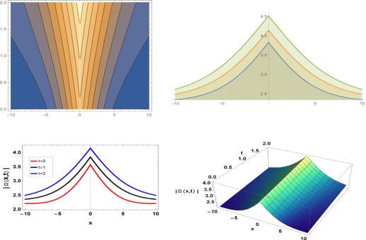
View original graphic|Download|PPT slide

Fig.1 Graph of (5.5) at $θ = 1, q = 0.1, c = 0.2, ϱ = 0.1$ .

View original graphic|Download|PPT slide

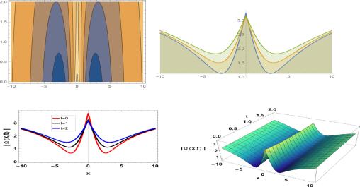
Fig.2 Graph of (5.6) at $θ = 1, q = 0.001, c = 0.8, ϱ = 0.001$ .

View original graphic|Download|PPT slide

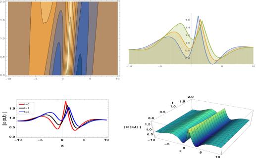
Fig.3 Graph of (5.20)using The new Kudryashov's method at $θ = 1, q = 0.5, c = 0.5, ϱ = 0.04$ .

View original graphic|Download|PPT slide

Fig.4 Graph of (5.21)using The new Kudryashov's method at $θ = 1, q = 0.4, c = 0.8, ϱ = 0.01$ .

View original graphic|Download|PPT slide

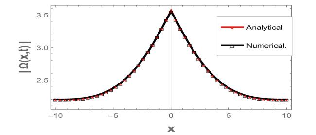
Fig.5 Comparison between the numerical results of (1.2) with the analytical solution (5.5) at $h = 0.2, k = 0.1, θ = 1, q = 0.01, c = 0.2, ϱ = 0.1$ .

View original graphic|Download|PPT slide

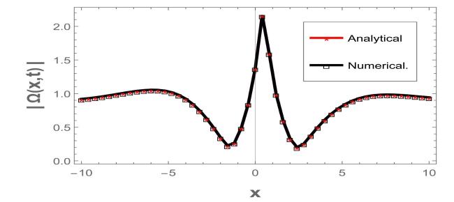
Fig.6 Comparison between the numerical results of (1.2) with the analytical solution (5.21) at $h = 0.2, k = 0.1, θ = 1, q = 0.4, c = 0.8, ϱ = 0.01$ .

8. Conclusion

Finally, we presented an extended tanh approach method to study the generalized

q

-deformed Sinh-Gordon equation. We have studied the model in this way and presented figures showing the correctness of what we hoped to reach from the proposed method. In addition, we presented an extensive numerical study of this model using the finite element method. In addition, the analytical solutions and the numerical solutions were compared. Through what we have reached, we can say that our results are a clear contribution to this field. At the end of our article, we present a future plan for our study, as we can solve more than one model in this way, and we can also develop other ways to solve different models. The proposed equation has opened up new possibilities for modeling physical systems in which symmetry has been compromised.

Declaration of Competing Interest

There is no conflict between the authors.

References

Publishing order | Descend order by publishing year | Descend order by cited within

[1]	G. Vilasi,J. Phys., 87 (2007), p. 012017 DOI: 10.1088/1742-6596/87/1/012017

[2]	S.D. Odintsov, V.K. Oikonomou,R. Myrzakulov. Symmetry, 14 (2022), p. 729 DOI: 10.3390/sym14040729

[3]	A. Goswami, J. Singh, D. Kumar, S. Gupta, Sushila. J. Ocean Eng. Sci., 4 (2) (2019), pp. 85-99

[4]	R.M. El-Shiekh, M. Gaballah. J. Ocean Eng. Sci., 5 (2) (2020), pp. 180-185

[5]	T. Islam, A. Akbar, H. Rezazadeh, A. Bekir. J. Ocean Eng. Sci. (2022), ISSN 2468-0133.

[6]	M. Cai, D. Li. Nonlinear Anal., 74 (13) (2011), pp. 4581-4588

[7]	A. Yusuf, T.A. Sulaiman, M. Mirzazadeh, K. Hosseini. Opt Quantum Electron., 53 (10) (2021), pp. 1-17

[8]	A.A. Kilbas, H.M. Srivastava, J.J. Trujillo, Theory and applications of fractional differential equations. Elsevier, Amsterdam (2006)

[9]	H. Durur, E. Ilhan,H. Bulut. Fractal Fract., 4 (3) (2020), p. 41 DOI: 10.3390/fractalfract4030041

[10]	H. Almusawa, K.A. Khalid, A.-M. Wazwaz, M. S. Mehanna, D. Baleanu, M. S. Osman,Results Phys., 31 (2021), p. 104933

[11]	K.A. Khalid, M. S. Mehanna,Results Phys., 28 (2021), p. 104596

[12]	K.A. Khalid, M. S. Mehanna. Opt,Quantum Electron., 53 (2021), p. 723

[13]	K.K. Ali, M. S. Mehanna. Alex, Eng. J., 60 (2021), pp. 5275-5285

[14]	A. Saha, K.A. Khalid, H. Rezazadeh,Y. Ghatani. Opt. Quantum Electron., 53 (2021), p. 150

[15]	A. Saha, K.A. Khalid, H. Rezazadeh,Y. Ghatani. Opt. Quantum Electron., 53 (2021), p. 150

[16]	A. Zafar, K.A. Khalid, M. Raheel, N. Jafar, K.S. Nisar. Eur.Phys, J.Plus, 135 (2020), p. 726

[17]	A. M. S. Mahdy. J. Ocean Eng. Sci. (2022), DOI:

[18]	A.M.S. Mahdy, K. Lotfy, W. Hassan, A.A. El-Bary, Waves Random Comp. Media, 31 (6) (2021), pp. 2040-2057 DOI: 10.1080/17455030.2020.1717673

[19]	M. Khader, N.H. Swetlam, A.M.S. Mahdy, Wseas Trans. Math., 13 (2014), pp. 31-38

[20]	A.M.S. Mahdy, K. Lotfy, A. El-Bary, H.H. Sarhan, Eur. Phy. J. Plus, 136 (5) (2021), pp. 1-17

[21]	S.B. GaziKarakoc, K.A. Khalid, Appl. Math. Comput., 371 (2020), p. 124933

[22]	A numerical. J. Ocean Eng. Sci., 3 (1) (2018), pp. 67-75

[23]	Ak Turgut S. Karakoc B. Gazi B, Anjan. J. Comput. Theor. Nanos., 13 (10) (2016), pp. 1-9

[24]	S.B. Karakoc, K.K. Ali. Comput, Methods Differ. Equ., 9 (3) (2021), pp. 670-691

[25]	International Bureau of Weights and Measures. SI Brochure: The International System of Units (SI) ( PDF) (9th ed.) (2020), p. 131 ISBN 978-92-822-2272-0.

[26]	H. Eleuch, Hindawi Adv. Math. Phys., 7 (2018), p. 5242757, DOI:

[27]	N. Raza, S. Arshed, H.I. Alrebdi, A.-H. Abdel-Aty,H. Eleuch. Results Phys., 35 (2022), p. 105358

[28]	T. Abdeljawad, D. Baleanu. Commun. Nonlinear Sci. Numer. Simul., 16 (12) (2011), pp. 4682-4688

[29]	R.P. Agarwal, Mathematical Proceedings of the Cambridge Philosophical Society, vol. 66, Cambridge University Press (1969), pp. 365-370

[30]	R.I. Butt, T. Abdeljawad, M.A. Alqudah, M.u. Rehman. J, Inequal. Appl., 2019 (1) (2019), pp. 1-13

[31]	M. Jleli, M. Mursaleen, B. Samet. Electron. J. Differ. Equ., 2016 (17) (2016), pp. 1-14

[32]	V.G. Kac, P. Cheung. Quantum calculus. Springer (2002), p. 113

[33]	K. Victor, C. Pokman, Q. calculus. Universitext. Springer-Verlag (2002) ISBN 0-387-95341-8.

[34]	K.A. Khalid, M. S. Mehanna. Opt,Quantum Electron., 53 (2021), p. 723

[35]	K.K. Ali, M. S. Mehanna. Alex, Eng. J., 60 (2021), pp. 5275-5285

[36]	K.R. Raslan,K.K. Ali. Nonlinear Eng., 9 (2020), pp. 432-448 DOI: 10.1515/nleng-2020-0027

[37]	K.R. Raslan, K.K. Ali, H.M.Y. Al-Bayatti. Appl. Math. Inf. Sci., 15 (5) (2021), pp. 599-611

[38]	K.R. Raslan, K.K. Ali, M.S. Mohamed, A.R. Hadhoud. Adv. Differ. Equ., 442 (1) (2021), p. 2021

[39]	K.R. Raslan, K.K. Ali, M.A. Shaalan, H.K. Al-Jeaid. Int. J, Appl. Comput. Math, 8 (2022), p. 91

Options

Outlines

模态框（Modal）标题

Abstract

Cite this article

1. Introduction

2. q-Calculus

3. Mathematical analysis of the model

4. The strategy of the extended tanh function method

5. The analytical solution for the model

6. The numerical solution for the model

6.1. The numerical results

Table 1 Comparison between the numerical results with the analytical solution.

Table 2 Comparison between the numerical results with the analytical solution.

7. Graphical illustrations

Fig.1 Graph of (5.5) at θ=1,q=0.1,c=0.2,ϱ=0.1 .

Fig.2 Graph of (5.6) at θ=1,q=0.001,c=0.8,ϱ=0.001 .

Fig.3 Graph of (5.20)using The new Kudryashov's method at θ=1,q=0.5,c=0.5,ϱ=0.04 .

Fig.4 Graph of (5.21)using The new Kudryashov's method at θ=1,q=0.4,c=0.8,ϱ=0.01 .

Fig.5 Comparison between the numerical results of (1.2) with the analytical solution (5.5) at h=0.2,k=0.1,θ=1,q=0.01,c=0.2,ϱ=0.1 .

Fig.6 Comparison between the numerical results of (1.2) with the analytical solution (5.21) at h=0.2,k=0.1,θ=1,q=0.4,c=0.8,ϱ=0.01 .

8. Conclusion

Declaration of Competing Interest

References

Links

Fig.1 Graph of (5.5) at $θ = 1, q = 0.1, c = 0.2, ϱ = 0.1$ .

Fig.2 Graph of (5.6) at $θ = 1, q = 0.001, c = 0.8, ϱ = 0.001$ .

Fig.3 Graph of (5.20)using The new Kudryashov's method at $θ = 1, q = 0.5, c = 0.5, ϱ = 0.04$ .

Fig.4 Graph of (5.21)using The new Kudryashov's method at $θ = 1, q = 0.4, c = 0.8, ϱ = 0.01$ .

Fig.5 Comparison between the numerical results of (1.2) with the analytical solution (5.5) at $h = 0.2, k = 0.1, θ = 1, q = 0.01, c = 0.2, ϱ = 0.1$ .

Fig.6 Comparison between the numerical results of (1.2) with the analytical solution (5.21) at $h = 0.2, k = 0.1, θ = 1, q = 0.4, c = 0.8, ϱ = 0.01$ .