Analytical solutions of simplified modified Camassa-Holm equation with conformable and M-truncated derivatives: A comparative study

Ismail Onder; Melih Cinar; Aydin Secer; Mustafa Bayram

doi:10.1016/j.joes.2022.06.012

Journal of Ocean Engineering and Science >

2024 , Vol. 9 >Issue 3: 240 - 250

DOI: https://doi.org/10.1016/j.joes.2022.06.012

Original article

Analytical solutions of simplified modified Camassa-Holm equation with conformable and M-truncated derivatives: A comparative study

Ismail Onder ^,^a ,
Melih Cinar ^,^a^,^b ,
Aydin Secer ^,^a^,^c ,
Mustafa Bayram ^,^c

Expand

^a Department of Mathematical Engineering, Yildiz Technical University, Istanbul, Turkey
^b Graduate School of Natural and Aplied Sciences, Yildiz Technical University, Istanbul, Turkey
^c Department of Computer Engineering, Biruni University, Istanbul, Turkey

^*E-mail addresses: ionder@yildiz.edu.tr (I. Onder),

mcinar@yildiz.edu.tr (M. Cinar),

asecer@yildiz.edu.tr (A. Secer),

mustafabayram@biruni.edu.tr (M. Bayram).

Received date: 2022-05-03

Revised date: 2022-06-04

Accepted date: 2022-06-06

Online published: 2024-08-17

Fold

Abstract

This paper extracts some analytical solutions of simplified modified Camassa-Holm (SMCH) equations with various derivative operators, namely conformable and M-truncated derivatives that have been recently introduced. The SMCH equation is used to model the unidirectional propagation of shallow-water waves. The extended rational sineâˆ’cosine and sinhâˆ’cosh techniques have been successfully implemented to the considered equations and some kinds of the solitons such as kink and singular have been derived. We have checked that all obtained solutions satisfy the main equations by using a computer algebraic system. Furthermore, some 2D and 3D graphical illustrations of the obtained solutions have been presented. The effect of the parameters in the solutions on the wave propagation has been examined and all figures have been interpreted. The derived solutions may contribute to comprehending wave propagation in shallow water. So, the solutions might help further studies in the development of autonomous ships/underwater vehicles and coastal zone management, which are critical topics in the ocean and coastal engineering.

Highlights

● Simplified modified Camassa-Holm equation with conformable and M- fractional derivative order is investigated.

● The novel solutions of considered equations are obtained analytically.

● The solutions of the conformable and $M -$ truncated model are graphically compared in the figures for different values of $α$ and $β$ that are in order of the derivative operator.

● The considered method suggests trigonometric functions producing dark, singular, and trigonometric solitons etc.

Key words： Modified Camassa-Holm equation; Conformable derivative; M- truncated derivative; Extended rational sine - cosine technique; Extended rational sinh − cosh technique; Exact solutions

Cite this article

Ismail Onder , Melih Cinar , Aydin Secer , Mustafa Bayram . Analytical solutions of simplified modified Camassa-Holm equation with conformable and M-truncated derivatives: A comparative study[J]. Journal of Ocean Engineering and Science, 2024 , 9(3) : 240 -250 . DOI: 10.1016/j.joes.2022.06.012

1. Introduction

Modeling the wave motions in shallow water waves has been one of the areas that attracted the attention of researchers in the last eight decades [1], [2]. The mathematical model of the motion of the waves as other real phenomena is commonly described by partial differential equations [3], [4], [5], [6], [7]. Some of the phenomenon wave equations are Korteweg-de-Vries [8], Benjamin-Bona-Mahony [9], Boussinesq-like [10], [11], [12], [13], Davey-Stewartson [14], Novikov-Veselov [15], Whitham [16], Kadomstev-Petviashvili [17]. Besides, Roberto Camassa and Darryl D. Holm introduced a completely integrable dispersive shallow-water equation in 1993 [18]:

(1)

Θ_{t} + 2 k Θ_{x} - Θ_{x x t} + 3 Θ Θ_{x} = 2 Θ_{x} Θ_{x x} + Θ Θ_{x x x},

where

Θ = Θ (x, t)

is the fluid velocity,

k

is a constant associated with the critical speed of wave of the shallow water. CH equation models the soliton interaction and wave breaking and is used for simulating shallow waters, coastal and harbors in ocean engineering [19], [20]. There are some studies on global conservative solutions of the Camassa-Holm (CH) equation [21], generalization of the equation [22], inverse scattering [23], conservation laws [24], long-time asymptotics [25], peakons of CH [26], finite propagation speed, [27] well-posedness, [28] etc. Besides, some researchers carried out some studies on the modifications and simplifications of the CH equation. In 2006, Abdul-Majid Wazwaz studied the modified Camassa-Holm (MCH) equation as follows [29]:

(2)

Θ_{t} - Θ_{x x t} + 3 Θ^{2} Θ_{x} - 2 Θ_{x} Θ_{x x} - Θ Θ_{x x x} = 0 .

As a result of simplifying the equation above, the simplified modified Camassa-Holm equation (SMCH) [30] is obtained:

(3)

Θ_{t} + 2 k Θ_{x} - Θ_{x x t} + ω Θ^{2} Θ_{x} = 0,

where

k

and

ω

are non-zero constants.

Fractional calculus has become quite well-known in a number of areas of science and engineering. It has been used to model a wide variety of dynamical processes and complicated nonlinear physical phenomena in the fields of physics, engineering, chemistry, viscoelasticity, and electromagnetics, etc [31], [32], [33], [34], [35]. This subject has risen to prominence in recent decades as a result of its extensive applicability in the aforementioned fields. Riemann-Liouville [36], [37], Caputo [38], and Caputo-Fabrizio [39] fractional derivative operators are the most frequently used operators in the literature. Besides, beta,

M -

truncated and conformable derivative operators have been introduced recently. There are some recent studies in the literature on conformable and M-truncated derivative models in ocean engineering field. These studies [40], [41], [42], [43] are about obtaining soliton solutions of the models with local derivatives. On the other hand, the number of articles in which these conformable and

M -

truncated derivative operators are used together and which are compared is very few. We believe that this study will help partially fill this gap in the literature. Therefore, it has become extremely important to solve the differential equations containing these kinds of derivatives analytically or numerically.

This paper mainly aims to derive the analytical solutions of the SMCH equations with conformable and M- truncated derivatives and compare the obtained solutions. To our best knowledge, an extended rational

s i n e - c o s i n e

and

s i n h - c o s h

methods [44], [45] have been successfully applied to MCH equation including various derivative operators for the first time. The considered methods were used for the perturbed nonlinear Schrodinger equation [44], Boussinesq-like equations, [46], nonlinear fractional

ϕ^{4}

function [47], coupled nonlinear Schrdinger equation [48], Hirota-Satsuma coupled KdV equation [49], coupled Maccaris system [50] and Radhakrishnan-Kundu-Lakshmanan equation [51]. Some studies on SMCH equation which we consider are modified simple equation method [30], exp-function method on the fractional type [52], Hes semi-inverse method [53], Darboux transformation and multi-soliton solution [54], exp

(- ϕ (η))

-expansion method [55], novel

(G^{'} / G)

expansion method [56], sine-gordon expansion method [57], new auxiliary method [58] and unified solver method [59].

The remaining parts of the article are organized as: Some preliminaries are considered in the Secton 2. The considered methods and their algorithms are dealt with in Section 3. In Section 4, the governing models with various derivative operators are presented. In Section 5, we apply the method to SMCH equation with different definitions of the derivatives and compare the results in 2D and 3D figures. The results and discussions are included in Section 6. The conclusion is given in the final section.

2. Preliminary information

2.1. Conformable derivative

Definition 2.1.1. Let

z : [0, \infty) \to R

be a function. Local conformable derivative of

z (y)

with

α

order is defined as follows [60]:

(4)

D_{y}^{α} (z (y)) = \lim_{h \to 0} \frac{z (y + h y^{1 - α}) - z (y)}{h},

where

α \in (0, 1], y > 0

Theorem 2.1.1 [60] Let

ϕ (y)

and

ψ (y)

α -

differentiable functions for

α \in (0, 1], y > 0

. Then,

(i)

D_{y}^{α} (m ϕ (y) + n ψ (y)) = m D_{y}^{α} ϕ (y) + n D_{y}^{α} ψ (y),

m, n \in R,

(ii)

D_{y}^{α} (y^{n}) = n y^{n - α}, n \in R

(iii) If

ϕ (y) = m

in which

m

is a constant, then

D_{y}^{α} (m) = 0,

(iv)

D_{y}^{α} (ψ (y) ϕ (y)) = ψ (y) D_{y}^{α} ϕ (y) + ϕ (y) D_{y}^{α} ψ (y),

(v)

D_{y}^{α} (\frac{ϕ (y)}{ψ (y)}) = \frac{ψ (y) D_{y}^{α} ϕ (y) - ϕ (y) D_{l}^{α} ψ (y)}{ψ^{2} (y)}, ψ (y) \neq 0,

(vi) If the first derivative of

ϕ (y)

exists, then

D_{y}^{α} (ϕ (y)) = y^{1 - α} \frac{d ϕ (y)}{d y} .

2.2. Local M-truncated derivative

Definition 2.2.1. The truncated Mittag-Leffler function (TMLF) is defined as follows [61]:

(5)

_{i} E_{β} (f) = \sum_{j = 0}^{i} \frac{f^{j}}{Γ (β j + 1)},

in which

β > 0

and

f \in C

Definition 2.2.2. Let

v : [0, \infty) \to R

be a function, the local M-truncated derivative of

v

of order

α \in (0, 1)

with respect to (w.r.t.)

y

is given [61]:

(6)

D_{M, y}^{α, β} v (y) = \lim_{h \to 0} \frac{v (y +_{i} E_{β} (h y^{- α})) - v (y)}{h},

in which

β, y > 0

and

_{i} E_{β} (\cdot)

is a TMLF.

Theorem 2.2.1 Let

v (y)

α

order differentiable function at

y_{0} > 0

where

α \in (0, 1]

and

β > 0

. Then,

v (y)

is continuous at

y_{0}

[61] .

Theorem 2.2.2 [61] Let

0 < α \leq 1, β > 0, r, s \in R

and

ϕ, ψ

α -

differentiable at a point

y > 0 .

Then,

(1)

D_{M, y}^{α, β} (r ϕ + s ψ) (y) = r D_{M, y}^{α, β} ϕ (y) + s D_{M, y}^{α, β} ψ (y)

where

r, s

are real constants,

(2)

D_{M, y}^{α, β} (ϕ ψ) (y) = ϕ (y) D_{M, y}^{α, β} ψ (y) + ψ (y) D_{M, y}^{α, β} ϕ (y),

(3)

D_{M, y}^{α, β} (\frac{ϕ}{ψ}) (y) = \frac{ϕ (y) D_{M, y}^{α, β} ψ (y) - ψ (y) D_{M, y}^{α, β} ϕ (y)}{ψ {(y)}^{2}},

(4)

D_{M, y}^{α, β} (\frac{ϕ}{ψ}) (y) = \frac{ϕ (y) D_{M, y}^{α, β} ψ (y) - ψ (y) D_{M, y}^{α, β} ϕ (y)}{ψ {(y)}^{2}},

(5) If

ϕ

is differentiable, then

D_{M, y}^{α, β} (ϕ) (y) = \frac{y^{1 - α}}{Γ (β + 1)} \frac{d ϕ (y)}{d y}

3. Analysis of the method

(i) Consider the general form of the conformable PDE:

(7)

F (D_{x}^{α} Θ, D_{t}^{α} Θ, D_{x}^{α} D_{t}^{α} Θ, \dots) = 0,

and the traveling wave transformation:

(8)

Θ (x, t) = Y (η), η = \frac{1}{α} (x^{α} - t^{α}) .

(ii) Consider the local M-truncated PDE in general form:

(9)

F (D_{M, x}^{α, β} Θ, D_{M, t}^{α, β} Θ, D_{M, x}^{α, β} D_{M, t}^{α, β} Θ, \dots) = 0,

and the traveling wave transformation:

(10)

Θ (x, t) = Y (η), η = \frac{Γ (1 + β)}{α} (x^{α} - t^{α}) .

where

Θ (x, t)

is the unknown function,

D_{*}^{α} Θ

and

D_{M, *}^{α, β} Θ

denote

α

order conformable and M-truncated derivative of

Θ

w.r.t.

* (x

t)

, respectively. Inserting the wave transformation in Eq. (8) into the PDE in Eq. (7) turns into the following nonlinear ODE in general form:

(11)

K (Y, Y^{'}, Y^{″}, \dots) = 0

where

Y

is the unknown functions of

η

and the superscripts

^{'}

represent ordinary differential operator

\frac{d}{d η}

**3.1. Extended rational sine − cosine technique**

Step 1: Assume that Eq. (11) has the solution as:

(12)

Y (η) = \frac{δ_{0} \sin (μ η)}{δ_{2} + δ_{1} \cos (μ η)}, \cos (μ η) \neq - \frac{δ_{2}}{δ_{1}},

(13)

Y (η) = \frac{δ_{0} \cos (μ η)}{δ_{2} + δ_{1} \sin (μ η)}, \sin (μ η) \neq - \frac{δ_{2}}{δ_{1}},

where

μ

is the wave number and

δ_{i}

are parameters to be found for

i = 0, 1, 2

Step 2: Substitute Eq. (12) or Eq. (13) to Eq. 11, collect the all terms including the same powers of

\cos (μ η)

\sin (μ η)

and then equate to zero the coefficients of trigonometric functions which are

\cos (μ η)

\sin (μ η)

gives a system of equations. When the system is solved, the unknowns (

δ_{0}, δ_{1}, δ_{2}

and

μ

) can be found.

Step 3: With substitution

δ_{0}, δ_{1}, δ_{2}

and

μ

to Eq. (12) or Eq. (13), the solutions of Eq. (11) can be found.

3.2. Extended rational $s i n h - c o s h$ technique

Step 1: Assume that Eq. (11) has the solution as:

(14)

Y (η) = \frac{δ_{0} \sinh (μ η)}{δ_{2} + δ_{1} \cosh (μ η)}, \cosh (μ η) \neq - \frac{δ_{2}}{δ_{1}},

(15)

Y (η) = \frac{δ_{0} \cosh (μ η)}{δ_{2} + δ_{1} \sinh (μ η)}, \sinh (μ η) \neq - \frac{δ_{2}}{δ_{1}} .

where

μ

is the wave number and

δ_{i}

are parameters to be found for

i = 0, 1, 2

Step 2: Substitute Eq. (12) or Eq. (13) to Eq. (11), collect the all terms including the same powers of

\cosh (μ η)

\sinh (μ η)

and then equate to zero the coefficients of trigonometric functions which are

\cosh (μ η)

\sinh (μ η)

gives a system of equations. When the system is solved, the unknowns (

δ_{0}, δ_{1}, δ_{2}

and

μ

) can be found.

Step 3:By substituting

δ_{0}, δ_{1}, δ_{2}, μ

and

η

to Eq. (14) or Eq. (15), the solutions of Eq. (11) can be found.

4. Governing model

In this section, we deal with the simplified modified Camassa-Holm equation (SMCH) w.r.t. different definitions of derivatives that are conformable and M-truncated [59]:

4.1. Conformable SMCH equation

Conformable SMCH equation can be written as follows [59]:

(16)

D_{t}^{α} Θ + λ D_{x}^{α} Θ - D_{x x t}^{3 α} Θ + ω D_{t}^{α} Θ^{3} = 0,

where

Θ = Θ (x, t)

and

λ, ω

are non-zero real parameters. We use following wave transformations:

(17)

Θ (x, t) = Y (η), η = \frac{x^{α}}{α} - γ \frac{t^{α}}{α} .

4.2. M-truncated SMCH equation

M-truncated SMCH equation can be written as follows [59]:

(18)

_{i} D_{M, t}^{α, β} Θ + λ_{i} D_{M, x}^{α, β} Θ -_{i} D_{M, x x t}^{3 α, β} Θ + ω_{i} D_{M, t}^{α, β} Θ^{3} = 0 .

For M-truncated derivative, we use the following wave transformations:

(19)

Θ (x, t) = Y (η), η = \frac{Γ (1 + β)}{α} (x^{α} - γ t^{α}) .

4.3. Solving the SMCH equations with conformable and M-truncated derivatives

Inserting the wave transformations in (17), (19) to the Eq. (16) and Eq. (18), respectively, we obtain the following nonlinear ODE:

(20)

γ Y^{″} (η) + ω Y^{3} (η) + (λ - γ) Y (η) = 0 .

5. Application

5.1. Conformable SMCH equation

5.1.1. Solving via extended rational $s i n e - c o s i n e$ technique

Let us suppose that the solutions of the Eq. (20) are:

(21)

Y (η) = \frac{δ_{0} \sin [μ η]}{δ_{2} + δ_{1} \cos [μ η]} .

Let us insert Eq. (21) into the Eq. (20) and collect all terms that includes the same power of

c o s {[μ η]}^{m}

, one can find the following algebraic equation system:

(22)

\begin{matrix} c o s {(μ η)}^{2} : & - δ_{1}^{2} δ_{0} γ + δ_{1}^{2} δ_{0} λ + δ_{0}^{3} (- ω) = 0, \\ c o s {(μ η)}^{1} : & 2 δ_{0} δ_{1} δ_{2} γ μ^{2} - 4 δ_{0} δ_{1} δ_{2} γ + 4 δ_{0} δ_{1} δ_{2} λ = 0, \\ c o s {(μ η)}^{0} : & 8 δ_{1}^{2} δ_{0} γ μ^{2} - 4 δ_{2}^{2} δ_{0} γ μ^{2} - δ_{1}^{2} δ_{0} γ - 4 δ_{2}^{2} δ_{0} γ \\ + δ_{1}^{2} δ_{0} λ + 4 δ_{2}^{2} δ_{0} λ + 3 δ_{0}^{3} ω = 0 . \end{matrix}

The set below can be derived when the system above is solved:

Set 1.

(23)

{μ = \pm \frac{\sqrt{γ - λ}}{\sqrt{2 γ}}, δ_{0} = \pm \frac{\sqrt{δ_{1}^{2} (λ - γ)}}{\sqrt{ω}}, δ_{1} = δ_{1}, δ_{2} = 0} .

Choosing the set 1, we get the solutions of Eq. (20) as:

(24)

Y_{1} (η) = \pm \frac{\sqrt{λ - γ}}{\sqrt{ω}} \tan [\frac{η \sqrt{γ - λ}}{\sqrt{2 γ}}] .

Considering set 1 and Eq. (24), one can derive:

(25)

Θ_{11} (x, t) = \frac{\sqrt{λ - γ}}{\sqrt{ω}} \tan [\frac{\frac{(x^{α} - γ t^{α})}{α} \sqrt{γ - λ}}{\sqrt{2 γ}}],

(26)

Θ_{12} (x, t) = - \frac{\sqrt{λ - γ}}{\sqrt{ω}} \tan [\frac{\frac{(x^{α} - γ t^{α})}{α} \sqrt{γ - λ}}{\sqrt{2 γ}}] .

The solutions exist for

ω (γ - λ) > 0

and

γ (γ - λ) > 0

Set 2.

(27)

{μ = \pm \frac{\sqrt{2} \sqrt{γ - λ}}{\sqrt{γ}}, δ_{0} = \pm \frac{\sqrt{δ_{1}^{2} (λ - γ)}}{\sqrt{ω}}, δ_{2} = δ_{2}, δ_{1} = \pm δ_{2}} .

Choosing the set 2, we get the solutions of Eq. (20) as:

(28)

Y_{2} (η) = \pm \frac{\sqrt{λ - γ}}{\sqrt{ω}} \frac{s i n [\frac{\sqrt{2} \sqrt{γ - λ}}{\sqrt{γ}} η]}{δ_{2} + δ_{1} \cos [\frac{\sqrt{2} \sqrt{γ - λ}}{\sqrt{γ}} η]} .

Considering set 2 and Eq. (28), one can derive:

(29)

Θ_{21} (x, t) = \frac{\sqrt{λ - γ}}{\sqrt{ω}} \frac{s i n [\frac{\sqrt{2} \sqrt{γ - λ}}{\sqrt{γ}} \frac{(x^{α} - γ t^{α})}{α}]}{1 + \cos [\frac{\sqrt{2} \sqrt{γ - λ}}{\sqrt{γ}} \frac{(x^{α} - γ t^{α})}{α}]},

(30)

Θ_{22} (x, t) = - \frac{\sqrt{λ - γ}}{\sqrt{ω}} \frac{s i n [\frac{\sqrt{2} \sqrt{γ - λ}}{\sqrt{γ}} \frac{(x^{α} - γ t^{α})}{α}]}{1 + \cos [\frac{\sqrt{2} \sqrt{γ - λ}}{\sqrt{γ}} \frac{(x^{α} - γ t^{α})}{α}]},

(31)

Θ_{23} (x, t) = - \frac{\sqrt{λ - γ}}{\sqrt{ω}} \frac{s i n [\frac{\sqrt{2} \sqrt{γ - λ}}{\sqrt{γ}} \frac{(x^{α} - γ t^{α})}{α}]}{1 - \cos [\frac{\sqrt{2} \sqrt{γ - λ}}{\sqrt{γ}} \frac{(x^{α} - γ t^{α})}{α}]},

(32)

Θ_{24} (x, t) = \frac{\sqrt{λ - γ}}{\sqrt{ω}} \frac{s i n [\frac{\sqrt{2} \sqrt{γ - λ}}{\sqrt{γ}} \frac{(x^{α} - γ t^{α})}{α}]}{1 - \cos [\frac{\sqrt{2} \sqrt{γ - λ}}{\sqrt{γ}} \frac{(x^{α} - γ t^{α})}{α}]} .

The solutions exist for

ω (γ - λ) > 0

and

γ (γ - λ) > 0

Suppose that the solutions of the Eq. (20) are:

(33)

Y (η) = \frac{δ_{0} \cos [μ η]}{δ_{2} + δ_{1} \sin [μ η]} .

Let us insert Eq. (33) into the Eq. (20) and collect all terms that includes the same power of

s i n {[μ η]}^{m}

, one can find the following algebraic equation system:

(34)

\begin{matrix} s i n {(μ η)}^{2} : & δ_{1}^{2} δ_{0} γ - δ_{1}^{2} δ_{0} λ + δ_{0}^{3} ω = 0, \\ s i n {(μ η)}^{1} : & 2 δ_{0} δ_{1} δ_{2} γ μ^{2} - 4 δ_{0} δ_{1} δ_{2} γ + 4 δ_{0} δ_{1} δ_{2} λ = 0, \\ s i n {(μ η)}^{0} : & 8 δ_{1}^{2} δ_{0} γ μ^{2} - 4 δ_{2}^{2} δ_{0} γ μ^{2} - δ_{1}^{2} δ_{0} γ - 4 δ_{2}^{2} δ_{0} γ \\ + δ_{1}^{2} δ_{0} λ + 4 δ_{2}^{2} δ_{0} λ + 3 δ_{0}^{3} ω = 0 . \end{matrix}

The set below can be derived when the system above is solved:

Set 3.

(35)

{μ = \pm \frac{\sqrt{γ - λ}}{\sqrt{2 γ}}, δ_{0} = \pm \frac{\sqrt{δ_{1}^{2} (λ - γ)}}{\sqrt{ω}}, δ_{1} = δ_{1}, δ_{2} = 0} .

Choosing the set 3, we get the solutions of Eq. (20) as:

(36)

Y_{3} (η) = \pm \frac{\sqrt{(λ - γ)}}{\sqrt{ω}} \cot [\frac{\sqrt{γ - λ}}{\sqrt{2 γ}} η] .

Considering set 3 and Eq. (36), one can derive:

(37)

Θ_{31} (x, t) = \frac{\sqrt{(λ - γ)}}{\sqrt{ω}} \cot [\frac{\sqrt{γ - λ}}{\sqrt{2 γ}} \frac{(x^{α} - γ t^{α})}{α}],

(38)

Θ_{32} (x, t) = - \frac{\sqrt{(λ - γ)}}{\sqrt{ω}} \cot [\frac{\sqrt{γ - λ}}{\sqrt{2 γ}} \frac{(x^{α} - γ t^{α})}{α}],

The solutions exist for

ω (γ - λ) > 0

and

γ (γ - λ) > 0

Set 4.

(39)

{μ = \pm \frac{\sqrt{2} \sqrt{γ - λ}}{\sqrt{γ}}, δ_{0} = \pm \frac{\sqrt{δ_{1}^{2} (λ - γ)}}{\sqrt{ω}}, δ_{2} = δ_{2}, δ_{1} = \pm δ_{2}} .

Choosing the set 4, we get the solutions of Eq. (20) as:

(40)

Y_{4} (η) = \pm \frac{\sqrt{(λ - γ)}}{\sqrt{ω}} \frac{\cos [\frac{\sqrt{2} \sqrt{γ - λ}}{\sqrt{γ}} η]}{δ_{2} \pm δ_{1} \sin [\frac{\sqrt{2} \sqrt{γ - λ}}{\sqrt{γ}} η]} .

Considering set 4 and Eq. (40), one can derive:

(41)

Θ_{41} (x, t) = \frac{\sqrt{(λ - γ)}}{\sqrt{ω}} \frac{\cos [\frac{\sqrt{2} \sqrt{γ - λ}}{\sqrt{γ}} \frac{(x^{α} - γ t^{α})}{α}]}{1 + \sin [\frac{\sqrt{2} \sqrt{γ - λ}}{\sqrt{γ}} \frac{(x^{α} - γ t^{α})}{α}]},

(42)

Θ_{42} (x, t) = - \frac{\sqrt{(λ - γ)}}{\sqrt{ω}} \frac{\cos [\frac{\sqrt{2} \sqrt{γ - λ}}{\sqrt{γ}} \frac{(x^{α} - γ t^{α})}{α}]}{1 + \sin [\frac{\sqrt{2} \sqrt{γ - λ}}{\sqrt{γ}} \frac{(x^{α} - γ t^{α})}{α}]},

(43)

Θ_{43} (x, t) = - \frac{\sqrt{(λ - γ)}}{\sqrt{ω}} \frac{\cos [\frac{\sqrt{2} \sqrt{γ - λ}}{\sqrt{γ}} \frac{(x^{α} - γ t^{α})}{α}]}{1 - \sin [\frac{\sqrt{2} \sqrt{γ - λ}}{\sqrt{γ}} \frac{(x^{α} - γ t^{α})}{α}]},

(44)

Θ_{44} (x, t) = \frac{\sqrt{(λ - γ)}}{\sqrt{ω}} \frac{\cos [\frac{\sqrt{2} \sqrt{γ - λ}}{\sqrt{γ}} \frac{(x^{α} - γ t^{α})}{α}]}{1 - \sin [\frac{\sqrt{2} \sqrt{γ - λ}}{\sqrt{γ}} \frac{(x^{α} - γ t^{α})}{α}]} .

The solutions exist for

ω (γ - λ) > 0

and

γ (γ - λ) > 0

5.1.2. Solving via extended rational $s i n h - c o s h$ technique

Let us suppose that the solutions of the Eq. (20) are:

(45)

Y (η) = \frac{δ_{0} \sinh [μ η]}{δ_{2} + δ_{1} \cosh [μ η]} .

Let us insert Eq. (45) into the Eq. (20) and collect all terms that includes the same power of

c o s h {[μ η]}^{m}

, one can find the following algebraic equation system:

(46)

\begin{matrix} c o s h {(μ η)}^{2} : & - δ_{1}^{2} δ_{0} γ + δ_{1}^{2} δ_{0} λ + δ_{0}^{3} ω = 0, \\ c o s h {(μ η)}^{1} : & - 2 δ_{0} δ_{1} δ_{2} γ μ^{2} - 4 δ_{0} δ_{1} δ_{2} γ + 4 δ_{0} δ_{1} δ_{2} λ = 0, \\ c o s h {(μ η)}^{0} : & - 8 δ_{1}^{2} δ_{0} γ μ^{2} + 4 δ_{2}^{2} δ_{0} γ μ^{2} - δ_{1}^{2} δ_{0} γ - 4 δ_{2}^{2} δ_{0} γ \\ + δ_{1}^{2} δ_{0} λ + 4 δ_{2}^{2} δ_{0} λ - 3 δ_{0}^{3} ω = 0 . \end{matrix}

The set below can be derived when the system above is solved:

Set 5.

(47)

{μ = \pm \frac{\sqrt{λ - γ}}{\sqrt{2 γ}}, δ_{0} = \pm \frac{δ_{1} \sqrt{γ - λ}}{\sqrt{ω}}, δ_{1} = δ_{1}, δ_{2} = 0} .

Choosing the set 5, we get the solutions of Eq. (20) as:

(48)

Y_{5} (η) = \pm \frac{\sqrt{γ - λ}}{\sqrt{ω}} \tanh [\frac{\sqrt{λ - γ}}{\sqrt{2 γ}} η] .

Considering set 5 and Eq. (48), one can derive:

(49)

Θ_{51} (x, t) = \frac{\sqrt{γ - λ}}{\sqrt{ω}} \tanh [\frac{\sqrt{λ - γ}}{\sqrt{2 γ}} \frac{(x^{α} - γ t^{α})}{α}],

(50)

Θ_{52} (x, t) = - \frac{\sqrt{γ - λ}}{\sqrt{ω}} \tanh [\frac{\sqrt{λ - γ}}{\sqrt{2 γ}} \frac{(x^{α} - γ t^{α})}{α}],

The solutions exist for

ω (γ - λ) > 0

and

γ (γ - λ) > 0

Set 6.

(51)

{μ = \pm \frac{\sqrt{2} \sqrt{λ - γ}}{\sqrt{γ}}, δ_{0} = \pm \frac{δ_{1} \sqrt{γ - λ}}{\sqrt{ω}}, δ_{1} = δ_{1}, δ_{2} = 0} .

Choosing the set 6, we get the solutions of Eq. (20) as:

(52)

Y_{6} (η) = \pm \frac{\sqrt{γ - λ}}{\sqrt{ω}} \frac{\sinh [\frac{\sqrt{2} \sqrt{λ - γ}}{\sqrt{γ}} η]}{δ_{2} \pm δ_{1} \cosh [\frac{\sqrt{2} \sqrt{λ - γ}}{\sqrt{γ}} η]} .

Considering set 6 and Eq. (52), one can derive:

(53)

Θ_{61} (x, t) = \frac{\sqrt{γ - λ}}{\sqrt{ω}} \frac{\sinh [\frac{\sqrt{2} \sqrt{λ - γ}}{\sqrt{γ}} \frac{(x^{α} - γ t^{α})}{α}]}{1 + \cosh [\frac{\sqrt{2} \sqrt{λ - γ}}{\sqrt{γ}} \frac{(x^{α} - γ t^{α})}{α}]},

(54)

Θ_{62} (x, t) = - \frac{\sqrt{γ - λ}}{\sqrt{ω}} \frac{\sinh [\frac{\sqrt{2} \sqrt{λ - γ}}{\sqrt{γ}} \frac{(x^{α} - γ t^{α})}{α}]}{1 + \cosh [\frac{\sqrt{2} \sqrt{λ - γ}}{\sqrt{γ}} \frac{(x^{α} - γ t^{α})}{α}]},

(55)

Θ_{63} (x, t) = - \frac{\sqrt{γ - λ}}{\sqrt{ω}} \frac{\sinh [\frac{\sqrt{2} \sqrt{λ - γ}}{\sqrt{γ}} \frac{(x^{α} - γ t^{α})}{α}]}{1 - \cosh [\frac{\sqrt{2} \sqrt{λ - γ}}{\sqrt{γ}} \frac{(x^{α} - γ t^{α})}{α}]},

(56)

Θ_{64} (x, t) = \frac{\sqrt{γ - λ}}{\sqrt{ω}} \frac{\sinh [\frac{\sqrt{2} \sqrt{λ - γ}}{\sqrt{γ}} \frac{(x^{α} - γ t^{α})}{α}]}{1 - \cosh [\frac{\sqrt{2} \sqrt{λ - γ}}{\sqrt{γ}} \frac{(x^{α} - γ t^{α})}{α}]} .

The solutions exist for

ω (γ - λ) > 0

and

γ (γ - λ) > 0

Suppose that the solutions of the Eq. (20) are:

(57)

Y (η) = \frac{δ_{0} \cosh [μ η]}{δ_{2} + δ_{1} \sinh [μ η]} .

Let us insert Eq. (57) into the Eq. (20) and collect all terms that includes the same power of

s i n h {[μ η]}^{m}

, one can find the following algebraic equation system:

(58)

\begin{matrix} s i n h {(μ η)}^{2} : & - δ_{1}^{2} δ_{0} γ + δ_{1}^{2} δ_{0} λ + δ_{0}^{3} ω = 0, \\ s i n h {(μ η)}^{1} : & - 2 δ_{0} δ_{1} δ_{2} γ μ^{2} - 4 δ_{0} δ_{1} δ_{2} γ + 4 δ_{0} δ_{1} δ_{2} λ = 0, \\ s i n h {(μ η)}^{0} : & 8 δ_{1}^{2} δ_{0} γ μ^{2} + 4 δ_{2}^{2} δ_{0} γ μ^{2} + δ_{1}^{2} δ_{0} γ - 4 δ_{2}^{2} δ_{0} γ \\ - δ_{1}^{2} δ_{0} λ + 4 δ_{2}^{2} δ_{0} λ + 3 δ_{0}^{3} ω = 0 . \end{matrix}

The set below can be derived when the system above is solved: Set 7.

(59)

{μ = \pm \frac{\sqrt{λ - γ}}{\sqrt{2 γ}}, δ_{0} = \pm \frac{a_{1} \sqrt{γ - λ}}{\sqrt{ω}}, δ_{1} = δ_{1}, a_{2} = 0} .

Choosing the set 7, we get the solutions of Eq. (20) as:

(60)

Y_{7} (η) = \pm \frac{\sqrt{γ - λ}}{\sqrt{ω}} \coth [\frac{\sqrt{λ - γ}}{\sqrt{2 γ}} η] .

Considering set 7 and Eq. (60), one can derive:

(61)

Θ_{71} (x, t) = \frac{\sqrt{γ - λ}}{\sqrt{ω}} \coth [\frac{\sqrt{λ - γ}}{\sqrt{2 γ}} \frac{(x^{α} - γ t^{α})}{α}],

(62)

Θ_{72} (x, t) = - \frac{\sqrt{γ - λ}}{\sqrt{ω}} \coth [\frac{\sqrt{λ - γ}}{\sqrt{2 γ}} \frac{(x^{α} - γ t^{α})}{α}] .

The solutions exist for

ω (γ - λ) > 0

and

γ (γ - λ) > 0

Set 8.

(63)

{μ = \pm \frac{\sqrt{2} \sqrt{λ - γ}}{\sqrt{γ}}, δ_{0} = \pm \frac{a_{1} \sqrt{γ - λ}}{\sqrt{ω}}, δ_{2} = δ_{2}, δ_{1} = \pm δ_{2} i} .

Choosing the set 8, we get the solutions of Eq. (20) as:

(64)

Y_{8} (η) = \pm \frac{\sqrt{γ - λ}}{\sqrt{ω}} \frac{\cosh [\frac{\sqrt{2} \sqrt{λ - γ}}{\sqrt{γ}} η]}{δ_{2} \pm δ_{1} i \sinh [\frac{\sqrt{2} \sqrt{λ - γ}}{\sqrt{γ}} η]} .

Considering set 8 and Eq. (64), one can derive:

(65)

Θ_{81} (x, t) = \frac{\sqrt{γ - λ}}{\sqrt{ω}} \frac{\cosh [\frac{\sqrt{2} \sqrt{λ - γ}}{\sqrt{γ}} \frac{(x^{α} - γ t^{α})}{α}]}{1 + i \sinh [\frac{\sqrt{2} \sqrt{λ - γ}}{\sqrt{γ}} \frac{(x^{α} - γ t^{α})}{α}]},

(66)

Θ_{82} (x, t) = - \frac{\sqrt{γ - λ}}{\sqrt{ω}} \frac{\cosh [\frac{\sqrt{2} \sqrt{λ - γ}}{\sqrt{γ}} \frac{(x^{α} - γ t^{α})}{α}]}{1 + i \sinh [\frac{\sqrt{2} \sqrt{λ - γ}}{\sqrt{γ}} \frac{(x^{α} - γ t^{α})}{α}]},

(67)

Θ_{83} (x, t) = - \frac{\sqrt{γ - λ}}{\sqrt{ω}} \frac{\cosh [\frac{\sqrt{2} \sqrt{λ - γ}}{\sqrt{γ}} \frac{(x^{α} - γ t^{α})}{α}]}{1 - i \sinh [\frac{\sqrt{2} \sqrt{λ - γ}}{\sqrt{γ}} \frac{(x^{α} - γ t^{α})}{α}]},

(68)

Θ_{84} (x, t) = \frac{\sqrt{γ - λ}}{\sqrt{ω}} \frac{\cosh [\frac{\sqrt{2} \sqrt{λ - γ}}{\sqrt{γ}} \frac{(x^{α} - γ t^{α})}{α}]}{1 - i \sinh [\frac{\sqrt{2} \sqrt{λ - γ}}{\sqrt{γ}} \frac{(x^{α} - γ t^{α})}{α}]} .

The solutions exist for

ω (γ - λ) > 0

and

γ (γ - λ) > 0

5.2. M-truncated SMCH equation

5.2.1. Solving via extended rational $s i n e - c o s i n e$ technique

Let us suppose that the solutions of the Eq. (20) are:

(69)

Y (η) = \frac{δ_{0} \sin [μ η]}{δ_{2} + δ_{1} \cos [μ η]} .

Let us insert Eq. (69) into the Eq. (20) and collect all terms that includes the same power of

c o s {[μ η]}^{m}

, one can find the following algebraic equation system:

(70)

\begin{matrix} c o s {(μ η)}^{2} : & - δ_{1}^{2} δ_{0} γ + δ_{1}^{2} δ_{0} λ + δ_{0}^{3} (- ω) = 0, \\ c o s {(μ η)}^{1} : & 2 δ_{0} δ_{1} δ_{2} γ μ^{2} - 4 δ_{0} δ_{1} δ_{2} γ + 4 δ_{0} δ_{1} δ_{2} λ = 0, \\ c o s {(μ η)}^{0} : & 8 δ_{1}^{2} δ_{0} γ μ^{2} - 4 δ_{2}^{2} δ_{0} γ μ^{2} - δ_{1}^{2} δ_{0} γ - 4 δ_{2}^{2} δ_{0} γ \\ + δ_{1}^{2} δ_{0} λ + 4 δ_{2}^{2} δ_{0} λ + 3 δ_{0}^{3} ω = 0 . \end{matrix}

The set below can be derived when the system above is solved: Set 1.

(71)

{μ = \pm \frac{\sqrt{γ - λ}}{\sqrt{2 γ}}, δ_{0} = \pm \frac{\sqrt{δ_{1}^{2} (λ - γ)}}{\sqrt{ω}}, δ_{1} = δ_{1}, δ_{2} = 0} .

Choosing the set 1, we get the solutions of Eq. (20) as:

(72)

Y_{1} (η) = \pm \frac{\sqrt{λ - γ}}{\sqrt{ω}} \tan [\frac{η \sqrt{γ - λ}}{\sqrt{2 γ}}] .

Considering set 1 and Eq. (72), one can derive:

(73)

Θ_{11} (x, t) = \frac{\sqrt{λ - γ}}{\sqrt{ω}} \tan [\frac{\sqrt{γ - λ}}{\sqrt{2 γ}} (\frac{Γ (β + 1) (x^{α} - γ t^{α})}{α})],

(74)

Θ_{12} (x, t) = - \frac{\sqrt{λ - γ}}{\sqrt{ω}} \tan [\frac{\sqrt{γ - λ}}{\sqrt{2 γ}} (\frac{Γ (β + 1) (x^{α} - γ t^{α})}{α})] .

The solutions exist for

ω (γ - λ) > 0

and

γ (γ - λ) > 0

Set 2.

(75)

{μ = \pm \frac{\sqrt{2} \sqrt{γ - λ}}{\sqrt{γ}}, δ_{0} = \pm \frac{\sqrt{δ_{1}^{2} (λ - γ)}}{\sqrt{ω}}, δ_{2} = δ_{2}, δ_{1} = \pm δ_{2}} .

Choosing the set 2, we get the solutions of Eq. (20) as:

(76)

Y_{2} (η) = \pm \frac{\sqrt{λ - γ}}{\sqrt{ω}} \frac{s i n [\frac{\sqrt{2} \sqrt{γ - λ}}{\sqrt{γ}} η]}{δ_{2} + δ_{1} \cos [\frac{\sqrt{2} \sqrt{γ - λ}}{\sqrt{γ}} η]} .

Considering set 2 and Eq. (76), one can derive:

(77)

Θ_{21} (x, t) = \frac{\sqrt{λ - γ}}{\sqrt{ω}} \frac{s i n [\frac{\sqrt{2} \sqrt{γ - λ}}{\sqrt{γ}} (\frac{Γ (β + 1) (x^{α} - γ t^{α})}{α})]}{1 + \cos [\frac{\sqrt{2} \sqrt{γ - λ}}{\sqrt{γ}} (\frac{Γ (β + 1) (x^{α} - γ t^{α})}{α})]},

(78)

Θ_{22} (x, t) = - \frac{\sqrt{λ - γ}}{\sqrt{ω}} \frac{s i n [\frac{\sqrt{2} \sqrt{γ - λ}}{\sqrt{γ}} (\frac{Γ (β + 1) (x^{α} - γ t^{α})}{α})]}{1 + \cos [\frac{\sqrt{2} \sqrt{γ - λ}}{\sqrt{γ}} (\frac{Γ (β + 1) (x^{α} - γ t^{α})}{α})]},

(79)

Θ_{23} (x, t) = - \frac{\sqrt{λ - γ}}{\sqrt{ω}} \frac{s i n [\frac{\sqrt{2} \sqrt{γ - λ}}{\sqrt{γ}} (\frac{Γ (β + 1) (x^{α} - γ t^{α})}{α})]}{1 - \cos [\frac{\sqrt{2} \sqrt{γ - λ}}{\sqrt{γ}} (\frac{Γ (β + 1) (x^{α} - γ t^{α})}{α})]},

(80)

Θ_{24} (x, t) = \frac{\sqrt{λ - γ}}{\sqrt{ω}} \frac{s i n [\frac{\sqrt{2} \sqrt{γ - λ}}{\sqrt{γ}} (\frac{Γ (β + 1) (x^{α} - γ t^{α})}{α})]}{1 - \cos [\frac{\sqrt{2} \sqrt{γ - λ}}{\sqrt{γ}} (\frac{Γ (β + 1) (x^{α} - γ t^{α})}{α})]} .

The solutions exist for

ω (γ - λ) > 0

and

γ (γ - λ) > 0

Suppose that the solutions of the Eq. 20 are:

(81)

Y (η) = \frac{δ_{0} \cos [μ η]}{δ_{2} + δ_{1} \sin [μ η]} .

Let us insert Eq. (81) into the Eq. (20) and collect all terms that includes the same power of

s i n {[μ η]}^{m}

, one can find the following algebraic equation system:

(82)

\begin{matrix} s i n {(μ η)}^{2} : & δ_{1}^{2} δ_{0} γ - δ_{1}^{2} δ_{0} λ + δ_{0}^{3} ω = 0, \\ s i n {(μ η)}^{1} : & 2 δ_{0} δ_{1} δ_{2} γ μ^{2} - 4 δ_{0} δ_{1} δ_{2} γ + 4 δ_{0} δ_{1} δ_{2} λ = 0, \\ s i n {(μ η)}^{0} : & 8 δ_{1}^{2} δ_{0} γ μ^{2} - 4 δ_{2}^{2} δ_{0} γ μ^{2} - δ_{1}^{2} δ_{0} γ - 4 δ_{2}^{2} δ_{0} γ \\ + δ_{1}^{2} δ_{0} λ + 4 δ_{2}^{2} δ_{0} λ + 3 δ_{0}^{3} ω = 0 . \end{matrix}

The set below can be derived when the system above is solved:

Set 3.

(83)

{μ = \pm \frac{\sqrt{γ - λ}}{\sqrt{2 γ}}, δ_{0} = \pm \frac{\sqrt{δ_{1}^{2} (λ - γ)}}{\sqrt{ω}}, δ_{1} = δ_{1}, δ_{2} = 0} .

Choosing the set 3, we get the solutions of Eq. (20) as:

(84)

Y_{3} (η) = \pm \frac{\sqrt{(λ - γ)}}{\sqrt{ω}} \cot [\frac{\sqrt{γ - λ}}{\sqrt{2 γ}} η] .

Considering set 3 and Eq. (84), one can derive:

(85)

Θ_{31} (x, t) = \frac{\sqrt{(λ - γ)}}{\sqrt{ω}} \cot [\frac{\sqrt{γ - λ}}{\sqrt{2 γ}} (\frac{Γ (β + 1) (x^{α} - γ t^{α})}{α})],

(86)

Θ_{32} (x, t) = - \frac{\sqrt{(λ - γ)}}{\sqrt{ω}} \cot [\frac{\sqrt{γ - λ}}{\sqrt{2 γ}} (\frac{Γ (β + 1) (x^{α} - γ t^{α})}{α})],

The solutions exist for

ω (γ - λ) > 0

and

γ (γ - λ) > 0

Set 4.

(87)

{μ = \pm \frac{\sqrt{2} \sqrt{γ - λ}}{\sqrt{γ}}, δ_{0} = \pm \frac{\sqrt{δ_{1}^{2} (λ - γ)}}{\sqrt{ω}}, δ_{2} = δ_{2}, δ_{1} = \pm δ_{2}} .

Choosing the set 4, we get the solutions of Eq. (20) as:

(88)

Y_{4} (η) = \pm \frac{\sqrt{(λ - γ)}}{\sqrt{ω}} \frac{\cos [\frac{\sqrt{2} \sqrt{γ - λ}}{\sqrt{γ}} η]}{δ_{2} \pm δ_{1} \sin [\frac{\sqrt{2} \sqrt{γ - λ}}{\sqrt{γ}} η]} .

Considering set 4 and Eq. (40), one can derive:

(89)

Θ_{41} (x, t) = \frac{\sqrt{(λ - γ)}}{\sqrt{ω}} \frac{\cos [\frac{\sqrt{2} \sqrt{γ - λ}}{\sqrt{γ}} (\frac{Γ (β + 1) (x^{α} - γ t^{α})}{α})]}{1 + \sin [\frac{\sqrt{2} \sqrt{γ - λ}}{\sqrt{γ}} (\frac{Γ (β + 1) (x^{α} - γ t^{α})}{α})]},

(90)

Θ_{42} (x, t) = - \frac{\sqrt{(λ - γ)}}{\sqrt{ω}} \frac{\cos [\frac{\sqrt{2} \sqrt{γ - λ}}{\sqrt{γ}} (\frac{Γ (β + 1) (x^{α} - γ t^{α})}{α})]}{1 + \sin [\frac{\sqrt{2} \sqrt{γ - λ}}{\sqrt{γ}} (\frac{Γ (β + 1) (x^{α} - γ t^{α})}{α})]},

(91)

Θ_{43} (x, t) = - \frac{\sqrt{(λ - γ)}}{\sqrt{ω}} \frac{\cos [\frac{\sqrt{2} \sqrt{γ - λ}}{\sqrt{γ}} (\frac{Γ (β + 1) (x^{α} - γ t^{α})}{α})]}{1 - \sin [\frac{\sqrt{2} \sqrt{γ - λ}}{\sqrt{γ}} (\frac{Γ (β + 1) (x^{α} - γ t^{α})}{α})]},

(92)

Θ_{44} (x, t) = \frac{\sqrt{(λ - γ)}}{\sqrt{ω}} \frac{\cos [\frac{\sqrt{2} \sqrt{γ - λ}}{\sqrt{γ}} (\frac{Γ (β + 1) (x^{α} - γ t^{α})}{α})]}{1 - \sin [\frac{\sqrt{2} \sqrt{γ - λ}}{\sqrt{γ}} (\frac{Γ (β + 1) (x^{α} - γ t^{α})}{α})]} .

The solutions exist for

ω (γ - λ) > 0

and

γ (γ - λ) > 0

5.2.2. Solving via extended rational $s i n h - c o s h$ technique

Assume that the solutions of the Eq. (20) are:

(93)

Y (η) = \frac{δ_{0} \sinh [μ η]}{δ_{2} + δ_{1} \cosh [μ η]} .

Let us insert Eq. (93) into the Eq. (20) and collect all terms that includes the same power of

c o s h {[μ η]}^{m}

, one can find the following algebraic equation system:

(94)

\begin{matrix} c o s h {(μ η)}^{2} : & - δ_{1}^{2} δ_{0} γ + δ_{1}^{2} δ_{0} λ + δ_{0}^{3} ω = 0, \\ c o s h {(μ η)}^{1} : & - 2 δ_{0} δ_{1} δ_{2} γ μ^{2} - 4 δ_{0} δ_{1} δ_{2} γ + 4 δ_{0} δ_{1} δ_{2} λ = 0, \\ c o s h {(μ η)}^{0} : & - 8 δ_{1}^{2} δ_{0} γ μ^{2} + 4 δ_{2}^{2} δ_{0} γ μ^{2} - δ_{1}^{2} δ_{0} γ - 4 δ_{2}^{2} δ_{0} γ \\ + δ_{1}^{2} δ_{0} λ + 4 δ_{2}^{2} δ_{0} λ - 3 δ_{0}^{3} ω = 0 . \end{matrix}

The set below can be derived when the system above is solved: Set 5.

(95)

{μ = \pm \frac{\sqrt{λ - γ}}{\sqrt{2 γ}}, δ_{0} = \pm \frac{δ_{1} \sqrt{γ - λ}}{\sqrt{ω}}, δ_{1} = δ_{1}, δ_{2} = 0} .

Choosing the set 5, we get the solutions of Eq. (20) as:

(96)

Y_{5} (η) = \pm \frac{\sqrt{γ - λ}}{\sqrt{ω}} \tanh [\frac{\sqrt{λ - γ}}{\sqrt{2 γ}} η] .

Considering set 5 and Eq. (96), one can derive:

(97)

Θ_{51} (x, t) = \frac{\sqrt{γ - λ}}{\sqrt{ω}} \tanh [\frac{\sqrt{λ - γ}}{\sqrt{2 γ}} (\frac{Γ (β + 1) (x^{α} - γ t^{α})}{α})],

(98)

Θ_{52} (x, t) = - \frac{\sqrt{γ - λ}}{\sqrt{ω}} \tanh [\frac{\sqrt{λ - γ}}{\sqrt{2 γ}} (\frac{Γ (β + 1) (x^{α} - γ t^{α})}{α})] .

The solutions exist for

ω (γ - λ) > 0

and

γ (γ - λ) > 0

Set 6.

(99)

{μ = \pm \frac{\sqrt{2} \sqrt{λ - γ}}{\sqrt{γ}}, δ_{0} = \pm \frac{δ_{1} \sqrt{γ - λ}}{\sqrt{ω}}, δ_{1} = δ_{1}, δ_{2} = 0} .

Choosing the set 6, we get the solutions of Eq. (20) as:

(100)

Y_{6} (η) = \pm \frac{\sqrt{γ - λ}}{\sqrt{ω}} \frac{\sinh [\frac{\sqrt{2} \sqrt{λ - γ}}{\sqrt{γ}} η]}{δ_{2} \pm δ_{1} \cosh [\frac{\sqrt{2} \sqrt{λ - γ}}{\sqrt{γ}} η]} .

Considering set 6 and Eq. (100), one can derive:

(101)

Θ_{61} (x, t) = \frac{\sqrt{γ - λ}}{\sqrt{ω}} \frac{\sinh [\frac{\sqrt{2} \sqrt{λ - γ}}{\sqrt{γ}} (\frac{Γ (β + 1) (x^{α} - γ t^{α})}{α})]}{1 + \cosh [\frac{\sqrt{2} \sqrt{λ - γ}}{\sqrt{γ}} (\frac{Γ (β + 1) (x^{α} - γ t^{α})}{α})]},

(102)

Θ_{62} (x, t) = - \frac{\sqrt{γ - λ}}{\sqrt{ω}} \frac{\sinh [\frac{\sqrt{2} \sqrt{λ - γ}}{\sqrt{γ}} (\frac{Γ (β + 1) (x^{α} - γ t^{α})}{α})]}{1 + \cosh [\frac{\sqrt{2} \sqrt{λ - γ}}{\sqrt{γ}} (\frac{Γ (β + 1) (x^{α} - γ t^{α})}{α})]},

(103)

Θ_{63} (x, t) = - \frac{\sqrt{γ - λ}}{\sqrt{ω}} \frac{\sinh [\frac{\sqrt{2} \sqrt{λ - γ}}{\sqrt{γ}} (\frac{Γ (β + 1) (x^{α} - γ t^{α})}{α})]}{1 - \cosh [\frac{\sqrt{2} \sqrt{λ - γ}}{\sqrt{γ}} (\frac{Γ (β + 1) (x^{α} - γ t^{α})}{α})]},

(104)

Θ_{64} (x, t) = \frac{\sqrt{γ - λ}}{\sqrt{ω}} \frac{\sinh [\frac{\sqrt{2} \sqrt{λ - γ}}{\sqrt{γ}} (\frac{Γ (β + 1) (x^{α} - γ t^{α})}{α})]}{1 - \cosh [\frac{\sqrt{2} \sqrt{λ - γ}}{\sqrt{γ}} (\frac{Γ (β + 1) (x^{α} - γ t^{α})}{α})]} .

The solutions exist for

ω (γ - λ) > 0

and

γ (γ - λ) > 0

. Suppose that the solutions of the Eq. (20) are:

(105)

Y (η) = \frac{δ_{0} \cosh [μ η]}{δ_{2} + δ_{1} \sinh [μ η]} .

Let us insert Eq. (105) into the Eq. (20) and collect all terms that includes the same power of

s i n h {[μ η]}^{m}

, one can find the following algebraic equation system:

(106)

\begin{matrix} s i n h {(μ η)}^{2} : & - δ_{1}^{2} δ_{0} γ + δ_{1}^{2} δ_{0} λ + δ_{0}^{3} ω = 0, \\ s i n h {(μ η)}^{1} : & - 2 δ_{0} δ_{1} δ_{2} γ μ^{2} - 4 δ_{0} δ_{1} δ_{2} γ + 4 δ_{0} δ_{1} δ_{2} λ = 0, \\ s i n h {(μ η)}^{0} : & 8 δ_{1}^{2} δ_{0} γ μ^{2} + 4 δ_{2}^{2} δ_{0} γ μ^{2} + δ_{1}^{2} δ_{0} γ - 4 δ_{2}^{2} δ_{0} γ \\ - δ_{1}^{2} δ_{0} λ + 4 δ_{2}^{2} δ_{0} λ + 3 δ_{0}^{3} ω = 0 . \end{matrix}

The set below can be derived when the system above is solved:

Set 7.

(107)

{μ = \pm \frac{\sqrt{λ - γ}}{\sqrt{2 γ}}, δ_{0} = \pm \frac{a_{1} \sqrt{γ - λ}}{\sqrt{ω}}, δ_{1} = δ_{1}, a_{2} = 0} .

Choosing the set 7, we get the solutions of Eq. (20) as:

(108)

Y_{7} (η) = \pm \frac{\sqrt{γ - λ}}{\sqrt{ω}} \coth [\frac{\sqrt{λ - γ}}{\sqrt{2 γ}} η] .

Considering set 7 and Eq. (108), one can derive:

(109)

Θ_{71} (x, t) = \frac{\sqrt{γ - λ}}{\sqrt{ω}} \coth [\frac{\sqrt{λ - γ}}{\sqrt{2 γ}} (\frac{Γ (β + 1) (x^{α} - γ t^{α})}{α})],

(110)

Θ_{72} (x, t) = - \frac{\sqrt{γ - λ}}{\sqrt{ω}} \coth [\frac{\sqrt{λ - γ}}{\sqrt{2 γ}} (\frac{Γ (β + 1) (x^{α} - γ t^{α})}{α})] .

The solutions exist for

ω (γ - λ) > 0

and

γ (γ - λ) > 0

Set 8.

(111)

{μ = \pm \frac{\sqrt{2} \sqrt{λ - γ}}{\sqrt{γ}}, δ_{0} = \pm \frac{a_{1} \sqrt{γ - λ}}{\sqrt{ω}}, δ_{2} = δ_{2}, δ_{1} = \pm δ_{2} i} .

Choosing the set 8, we get the solutions of Eq. (20) as:

(112)

Y_{8} (η) = \pm \frac{\sqrt{γ - λ}}{\sqrt{ω}} \frac{\cosh [\frac{\sqrt{2} \sqrt{λ - γ}}{\sqrt{γ}} η]}{δ_{2} \pm δ_{1} i \sinh [\frac{\sqrt{2} \sqrt{λ - γ}}{\sqrt{γ}} η]} .

Considering set 8 and Eq. (112), one can derive:

(113)

Θ_{81} (x, t) = \frac{\sqrt{γ - λ}}{\sqrt{ω}} \frac{\cosh [\frac{\sqrt{2} \sqrt{λ - γ}}{\sqrt{γ}} (\frac{Γ (β + 1) (x^{α} - γ t^{α})}{α})]}{1 + i \sinh [\frac{\sqrt{2} \sqrt{λ - γ}}{\sqrt{γ}} (\frac{Γ (β + 1) (x^{α} - γ t^{α})}{α})]},

(114)

Θ_{82} (x, t) = - \frac{\sqrt{γ - λ}}{\sqrt{ω}} \frac{\cosh [\frac{\sqrt{2} \sqrt{λ - γ}}{\sqrt{γ}} (\frac{Γ (β + 1) (x^{α} - γ t^{α})}{α})]}{1 + i \sinh [\frac{\sqrt{2} \sqrt{λ - γ}}{\sqrt{γ}} (\frac{Γ (β + 1) (x^{α} - γ t^{α})}{α})]},

(115)

Θ_{83} (x, t) = - \frac{\sqrt{γ - λ}}{\sqrt{ω}} \frac{\cosh [\frac{\sqrt{2} \sqrt{λ - γ}}{\sqrt{γ}} (\frac{Γ (β + 1) (x^{α} - γ t^{α})}{α})]}{1 - i \sinh [\frac{\sqrt{2} \sqrt{λ - γ}}{\sqrt{γ}} (\frac{Γ (β + 1) (x^{α} - γ t^{α})}{α})]},

(116)

Θ_{84} (x, t) = \frac{\sqrt{γ - λ}}{\sqrt{ω}} \frac{\cosh [\frac{\sqrt{2} \sqrt{λ - γ}}{\sqrt{γ}} (\frac{Γ (β + 1) (x^{α} - γ t^{α})}{α})]}{1 - i \sinh [\frac{\sqrt{2} \sqrt{λ - γ}}{\sqrt{γ}} (\frac{Γ (β + 1) (x^{α} - γ t^{α})}{α})]} .

The solutions exist for

ω (γ - λ) > 0

and

γ (γ - λ) > 0

6. Results and discussion

In this paper, the powerful

s i n e - c o s i n e

and

s i n h - c o s h

techniques have been used for obtaining some analytical solutions of the SMCH equations with two new kinds of derivative operators which are conformable and M-truncated. A variety of solutions have been obtained using the methods and the derived solutions for two different derivative operators have been compared in

3 D

and

2 D

graphics by using Mathematica 12.

In Fig. 1, we depict the 3D and 2D graphs of the solutions

Θ_{24} (x, t)

of the conformable and M-truncated SMCH equation. In Fig. 1a, 3D comparison between Eq. (32) (conformable) and Eq. (80) (M-truncated) are plotted in three dimensional for

α = 0.5

and

β = 0.6

. In Fig. 1b, we present a 2D comparison between the conformable solution with

α = 0.7

and M-truncated solution with

α = 0.7, β = 0.4

for SMCH equation. The solution

Θ_{24} (x, t)

in Fig. 1 demonstrates a singular-periodic solution.

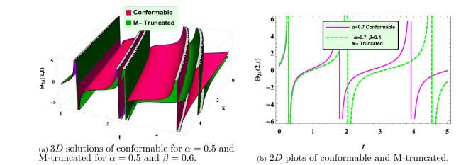
View original graphic|Download|PPT slide

Fig.1 Comparison of solutions of conformable in Eq. (32) and M-truncated derivative in Eq. (80) with $γ = 4, λ = 2,$ and $ω = - 3$ (Singular-periodic solution).

In Fig. 2, we depict the 3D and 2D graphs of the solutions

Θ_{51} (x, t)

. For SMCH equation with conformable derivative, the solutions

Θ_{51} (x, t)

are given in Eq. (49) and the solutions

Θ_{51} (x, t)

are given in Eq. (97) for SMCH equation with M-truncated derivative. In Fig. 2a, comparison between Eq. (49) and Eq. (97) are plotted in three dimensional for

α = 0.4

and

β = 0.6

. In Fig. 2b, we depicted the 2D plots of the solution with

γ = 0.7

λ = 70

ω = - 0.2

α = 0.4

for conformable solution and

α = 0.4, β = 0.6

for solutions for SMCH with M-truncated derivative solution of

Θ_{51} (x, t)

. The solution

Θ_{51} (x, t)

in Fig. 2 represents a kink solution.

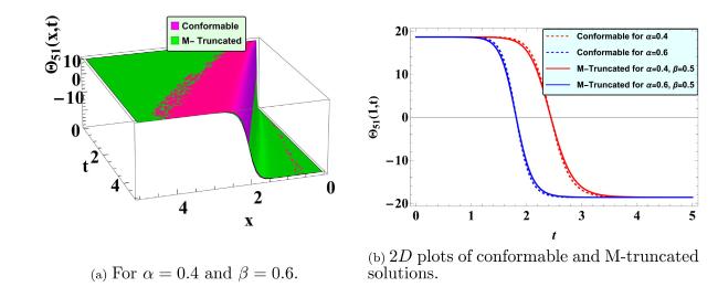
View original graphic|Download|PPT slide

Fig.2 Comparison of solutions of conformable in Eq. (49) and M-truncated derivative in Eq. (97) with $γ = 0.7, λ = 70,$ and $ω = - 0.2$ (Kink soliton).

Fig. 3 shows the effects of changing of the parameters on the wave propagation. In Fig. 2b, we illustrate the effect of the

ω

parameter on M-truncated and conformable, respectively. The parameters

ω = - 0.2, - 0.3, - 0.4

and fixed

γ = 0.7

λ = 70

are used for the solution

Θ_{51} (x, t)

in (49), (97) where

α = 0.4

β = 0.5

. Since the parameter

ω

is in the denominator of the obtained solutions, the wave amplitude increases when

ω

decreases. In Fig. 2, Fig. 3 a, we demonstrate the effect of the

γ

parameter on M-truncated and conformable, respectively where

γ = 0.7, 0.8, 0.9

and fixed

ω = - 0.2

λ = 70

. When the parameter

γ

increases, the wave moves to the left along the t-axis. In Fig. 3c, we give the effect of the parameter

λ

on solutions with M-truncated and conformable, respectively where

λ = 70, 80, 90

and fixed

ω = - 0.2

γ = 0.7

. There are a positive correlation between the parameter

λ

and the wave amplitude.

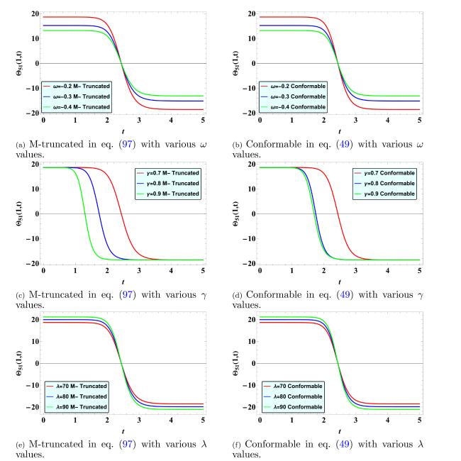
View original graphic|Download|PPT slide

Fig.3 The effects of the parameters to solutions Conformable in Eq. (49) with M-truncated and Eq. (97) with fixed $α = 0.4$ and $β = 0.6$ (Kink soliton).

In Fig. 4, the some plots of the solutions

Θ_{64} (x, t)

are illustrated. For SMCH equation with conformable derivative, the solutions

Θ_{64} (x, t)

are given in Eq. (56) and the solutions

Θ_{64} (x, t)

are given in Eq. (104) for SMCH equation with M-truncated derivative. Fig. 4a shows the 3D plots of the conformable with

α = 0.5

and solutions for SMCH with M-truncated derivative with

α = 0.5, β = 0.6

. The solution is known as singular solution. Fig. 4b shows the 2D plots of conformable with

α = 0.4, 0.5

and solutions for SMCH with M-truncated derivative with fixed

β = 0.1

and

α = 0.4, 0.5

. The figure of the solution

Θ_{64} (x, t)

illustrates a singular solution.

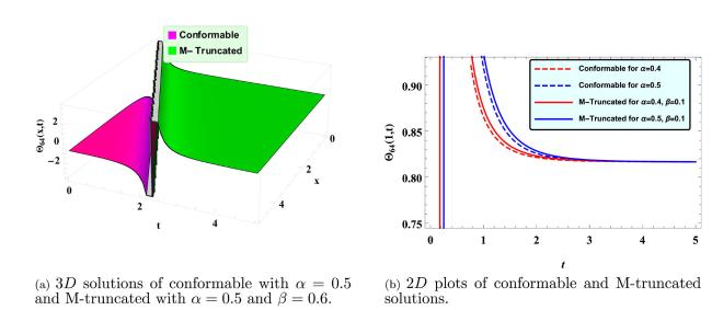
View original graphic|Download|PPT slide

Fig.4 Comparison of solutions of conformable in Eq. (56) and M-truncated derivative in Eq. (104) with $γ = 2, λ = 4,$ and $ω = - 3$ (Singular solution).

In Fig. 5, we present the three-dimensional and two-dimensional graphs of the solution

Θ_{71} (x, t)

. In Fig. 5a, we depict the 2D plots of solutions in Eq. (109) for SMCH with M-truncated derivative where

α = 0.5

and various

β = 1, 2, 3

and

β = 4

. Fig. 5a represents a comparison between the solutions

Θ_{71} (x, t)

of SMCH equations with the conformable and M-truncated derivative. Fig. 5b shows that the solutions of SMCH equations with the conformable and M-truncated derivative overlap for

β = 1

. The solution

Θ_{71} (x, t)

represent a singular solution.

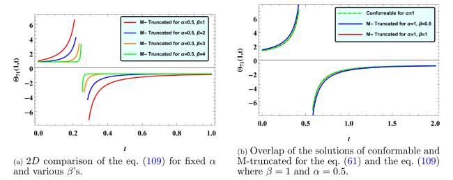
View original graphic|Download|PPT slide

Fig.5 Various 2D comparisons where $γ = 2, λ = 4,$ and $ω = - 3 .$

In [58], the SMCH equation with classical derivative was studied and some closed-form wave solutions for the equation were derived. When our results are compared with the reference [58], our solutions in more general solutions than the solutions in the reference. Because we have used the models with the conformable and M-truncated, which are one of the general forms of the classical derivative. In addition, our method is powerful and effective such that it presents many solutions which include kinds of solitons. Also, our study is one of the rare studies examining the effect of these two local derivative operators on the same model. Not only the effect of the operators is examined, but also the effect of the parameters in the model on the wave motion. We expect that our results might be helpful for future studies in ocean engineering and science.

The figures include various kinds of solitons and simulate the propagation and breaking of shallow water waves in oceans, lakes, and rivers. Understanding the wave propagation and interactions contributes to important topics in the ocean and coastal engineering such as the development of autonomous ships/underwater vehicles and designing coastal defense schemes, which the engineers must consider. So, it is expected that the results might be helpful for the ocean and coastal engineering.

7. Conclusion

In this paper, we have dealt with the SMCH including conformable or M-truncated derivatives instead of the model with the classical derivative, which has been commonly studied in the literature. We have applied the extended rational

s i n e - c o s i n e

and

s i n h - c o s h

methods to construct analytical solutions for SMCH equation modeling the unidirectional propagation of shallow-water waves. As a main contribution of the work, a variety of exact solutions for the SMCH equation with various derivative operators have been successfully extracted in the rational forms of trigonometric and hyperbolic functions. Some of the obtained solutions using the considered methods have been compared in 3D surface and 2D line plots. In the figures, the effect of the used different derivative operators in the SMCH equations has been illustrated. It can be deduced that M- truncated derivative is reduced to conformable derivative when

β = 1,

and it is reduced to classical derivative for

β = α = 1 .

The derived result shows that the techniques are efficient and easily applicable for producing analytical solutions of non-linear PDEs, including various kinds of derivatives. The obtained solutions might help further studies in the development of autonomous ships/underwater vehicles and coastal zone management, which are critical topics in the ocean and coastal engineering.

Declaration of Competing Interest

Authors declare that there is no conflict of interest whatsoever.

Acknowledgment

The second author (MC) would like to thank the Scientific and Technological Research Council of Turkey (TUBITAK) for the financial support of the 2211-A Fellowship Program.

References

Publishing order | Descend order by publishing year | Descend order by cited within

[1]	R.F. Dressler. Commun. Pure Appl. Math., 2 (2-3) (1949), pp. 149-194, DOI:

[2]	G.F. Carrier, H.P. Greenspan. J, Fluid Mech., 4 (1) (1958), pp. 97-109, DOI:

[3]	M. Cinar, I. Onder, A. Secer, A. Yusuf, T.A. Sulaiman, M. Bayram, H. Aydin. Int. J, Appl. Comput. Math., 7 (4) (2021), pp. 1-17, DOI:

[4]	H.M. Baskonus, A.A. Mahmud, K.A. Muhamad,T. Tanriverdi. Math. Methods Appl. Sci. (2022), DOI:

[5]	M. Ozisik, M. Cinar, A. Secer,M. Bayram. Optik, 261 (2022), p. 169202, DOI: https://www.sciencedirect.com/science/article/pii/S0030402622005551/pdfft?md5=953a3bbe9d4ac0c0e1aedc41cb02fdad&pid=1-s2.0-S0030402622005551-main.pdf

[6]	Q. Chen, H.M. Baskonus, W. Gao, E. Ilhan. Alexandria Eng. J., 61 (10) (2022), pp. 7843-7851, DOI: https://www.sciencedirect.com/science/article/pii/S111001682200031X/pdfft?md5=9e41a5a2e9c59b1f71e8a8aef4df959f&pid=1-s2.0-S111001682200031X-main.pdf

[7]	M. Cinar, I. Onder, A. Secer, M. Bayram, T. Abdulkadir Sulaiman, A. Yusuf, Waves Random Complex Medium (2022), pp. 1-14, DOI:

[8]	R. Hirota, Phys. Rev. Lett., 27 (18) (1971), pp. 1192-1194, DOI:

[9]	B. Benjamin, J. Bona, J. Mahony. Philos. Trans. R. Soc. Lond. Ser. A Math. Phys. Sci., 272 (1220) (1972), pp. 47-78, DOI:

[10]	H. Rezazadeh, M.S. Osman, M. Eslami, M. Mirzazadeh, Q. Zhou, S.A. Badri, A. Korkmaz. Nonlinear Eng., 8 (1) (2019), pp. 224-230, DOI:

[11]	L. Akinyemi, M. Åženol, U. Akpan,H. Rezazadeh. J. Ocean Eng. Sci. (2022), DOI:

[12]	S. Kumar, S. Malik, H. Rezazadeh, L. Akinyemi. Nonlinear Dyn., 107 (3) (2022), pp. 2703-2716, DOI:

[13]	H. Esen, N. Ozdemir, A. Secer,M. Bayram. J. Ocean Eng. Sci. (2022), DOI:

[14]	A. Davey, K. Stewartson. Proc. R. Soc. Lond. A. Math. Phys. Sci., 338 (1613) (1974), pp. 101-110, DOI:

[15]	S.P. Novikov, A.P. Veselov, Physica D, 18 (1) (1986), pp. 267-273, DOI: https://www.sciencedirect.com/science/article/pii/0167278986901879/pdf?md5=f339dd01f6d4593a8ef92ccbc0a54919&pid=1-s2.0-0167278986901879-main.pdf

[16]	B. Fornberg, W.G. Beresford. Philos. Trans. R. Soc. Lond. Ser. A Math. Phys. Sci., 289 (1361) (1978), pp. 373-404, DOI:

[17]	B.B. Kadomtsev, V.I. Petviashvili, B.B. Kadomtsev, V.I. Petviashvili, SPhD, 15 (1970), p. 539

[18]	R. Camassa, D.D. Holm. Phys. Rev, Lett., 71 (11) (1993), pp. 1661-1664, DOI:

[19]	A. Bekir, Ã-. GÃ¼ner. Ocean Eng., 74 (2013), pp. 276-279, DOI: https://www.sciencedirect.com/science/article/pii/S0029801813003715/pdfft?md5=ffc9574861a32ef6db0271a9999dd097&pid=1-s2.0-S0029801813003715-main.pdf

[20]	A. Kurt, Appl. Ocean Res., 85 (2019), pp. 128-135, DOI: https://www.sciencedirect.com/science/article/pii/S0141118718307429/pdfft?md5=8e200e38ddbd4c534c04ee606822f184&pid=1-s2.0-S0141118718307429-main.pdf

[21]	A. Bressan, A. Constantin, equation (2007), DOI:

[22]	V. Novikov. J. Phys, A: Math. Theor., 42 (34) (2009), p. 14, DOI:

[23]	A. Constantin, V.S. Gerdjikov, R.I. Ivanov, Inverse Probl., 22 (6) (2006), pp. 2197-2207, DOI:

[24]	J. Lenells. J. Phys, A Math. Gen., 38 (4) (2005), pp. 869-880, DOI:

[25]	A.B. De Monvel, A. Kostenko, D. Shepelsky, G. Teschl. SIAM J. Math. Anal., 41 (4) (2009), pp. 1559-1588, DOI:

[26]	Z. Liu, T. Qian. Appl. Math. Model., 26 (3) (2002), pp. 473-480, DOI: https://www.sciencedirect.com/science/article/pii/S0307904X01000865/pdfft?md5=7b7c08fe1cf2a457819ba27bb70f30b3&pid=1-s2.0-S0307904X01000865-main.pdf

[27]	A. Constantin. J. Math, Phys., 46 (2) (2005), p. 023506, DOI:

[28]	R. Danchin, J. Differ. Equ., 192 (2) (2003), pp. 429-444, DOI: https://www.sciencedirect.com/science/article/pii/S0022039603000962/pdfft?md5=26512d8166dcb42cc7257ea9be13f4c7&pid=1-s2.0-S0022039603000962-main.pdf

[29]	A.M. Wazwaz, Phys. Lett. Sect. A, 352 (6) (2006), pp. 500-504, DOI: https://www.sciencedirect.com/science/article/pii/S0375960105019109/pdfft?md5=cd8f68b9b6606b216dfe909cb736bc57&pid=1-s2.0-S0375960105019109-main.pdf

[30]	M.N. Islam, M. Asaduzzaman, M.S. Ali. AIMS Math., 5 (1) (2019), pp. 26-41, DOI:

[31]	M. Cinar, A. Secer, M. Bayram. Alexandria Eng. J., 60 (6) (2021), pp. 5331-5340, DOI: https://www.sciencedirect.com/science/article/pii/S1110016821002799/pdfft?md5=b1a0fc2559e7591d825d4ad741499d1a&pid=1-s2.0-S1110016821002799-main.pdf

[32]	F. Ciuchi, A. Mazzulla, N. Scaramuzza, E.K. Lenzi, L.R. Evangelista. J, Phys. Chem. C, 116 (15) (2012), pp. 8773-8777, DOI:

[33]	S. Ullah, M.A. Khan, M. Farooq. Eur. Phys, J. Plus, 133 (6) (2018), pp. 1-14, DOI: https://www.sciencedirect.com/science/article/pii/S0169809518302709/pdfft?md5=f2436cb74205649a7307e1626a6d1b05&pid=1-s2.0-S0169809518302709-main.pdf

[34]	X. Wang, H. Qi, B. Yu, Z. Xiong, H. Xu. Commun, Nonlinear Sci. Numer. Simul., 50 (2017), pp. 77-87, DOI: https://www.sciencedirect.com/science/article/pii/S1007570417300667/pdfft?md5=359c0eca5691c2da0a43262d0c00f77b&pid=1-s2.0-S1007570417300667-main.pdf

[35]	A. Secer, M. Cinar. Therm. Sci., 24 (Suppl. 1) (2020), pp. 119-129

[36]	J.K. Hale, S.M.V. Lunel, Springer, New York, NY, USA (1993)

[37]	I. Podlubny, Academic Press, Cambridge, MA, USA (1998)

[38]	M. Caputo, Annali dell'Universit di Ferrara, 41 (1) (1995), pp. 73-84, DOI:

[39]	M. Caputo, M. Fabrizio. Progr. Fract. Differ. Appl., 1 (2) (2015), pp. 73-85

[40]	A. Tripathy, S. Sahoo, H. Rezazadeh, H. Ahmad,M. Inc. J. Ocean Eng. Sci. (2022), DOI:

[41]	L. Akinyemi, M. Åženol, O. Tasbozan, A. Kurt. J. Ocean Eng. Sci. (2021)

[42]	H. Ã‡erdik Yaslan, A. Girgin. J. Ocean Eng. Sci., 6 (3) (2021), pp. 228-236, DOI: https://www.sciencedirect.com/science/article/pii/S2468013320300966/pdfft?md5=8a2abb0445d52a7ec610b2b9a54a4eec&pid=1-s2.0-S2468013320300966-main.pdf

[43]	R. Hussain, A. Imtiaz, T. Rasool, H. Rezazadeh,M. Inc. J. Ocean Eng. Sci. (2022), DOI:

[44]	N. Mahak, G. Akram. Eur. Phys, J. Plus, 134 (4) (2019), pp. 1-10, DOI:

[45]	M. Cinar, I. Onder, A. Secer, M. Bayram, A. Yusuf, T.A. Sulaiman, M. Cinar, I. Onder, A. Secer, M. Bayram, A. Yusuf, T.A. Sulaiman. Electr. Res, Arch., 30 (1) (2022), pp. 335-361, DOI:

[46]	M.T. Darvishi, M. Najafi, A.M. Wazwaz, Waves Random Complex Medium, 30 (1) (2020), pp. 5-26, DOI:

[47]	N. Mahak, G. Akram. Phys. Scr., 94 (11) (2019), p. 115212, DOI:

[48]	T.A. Sulaiman, H. Bulut. Commun. Theor. Phys., 72 (2) (2020), p. 025003, DOI:

[49]	M. Alquran, I. Jaradat, D. Baleanu. Chin. J. Phys., 58 (2019), pp. 49-56, DOI: https://www.sciencedirect.com/science/article/pii/S0577907318312942/pdfft?md5=09f9f3a6afae180b9e16bf1a8aef410f&pid=1-s2.0-S0577907318312942-main.pdf

[50]	J. Vahidi, S.M. Zekavatmand, H. Rezazadeh, M. Inc, M.A. Akinlar,Y.M. Chu. Results Phys., 21 (2021), p. 103801, DOI: https://www.sciencedirect.com/science/article/pii/S2211379720322075/pdfft?md5=9820086ec6439a471a5415cc9cd9f34c&pid=1-s2.0-S2211379720322075-main.pdf

[51]	S. ur Rehman, J. Ahmad. Alexandria Eng. J., 60 (1) (2021), pp. 1339-1354, DOI:

[52]	A. Zulfiqar, J. Ahmad. Alexandria Eng. J., 59 (5) (2020), pp. 3565-3574, DOI: https://www.sciencedirect.com/science/article/pii/S1110016820302544/pdfft?md5=db81924c2ebb82376effbdcd3b11dfac&pid=1-s2.0-S1110016820302544-main.pdf

[53]	M. Najafi, S. Arbabi, M. Najafi. Int. J. Phys. Res., 1 (1) (2013), pp. 1-6 DOI: 10.1109/IranianCEE.2013.6599548

[54]	B. Xia, R. Zhou, Z. Qiao. J. Math. Phys., 57 (10) (2016), p. 103502, DOI:

[55]	A. Ali, M.A. Iqbal, S.T. Mohyud-Din. Egypt. J, Basic Appl. Sci., 3 (2) (2016), pp. 134-140, DOI: https://www.sciencedirect.com/science/article/pii/S2314808X16000038/pdfft?md5=0106548635831c5480deba1ebf3bbbb8&pid=1-s2.0-S2314808X16000038-main.pdf

[56]	M. Shakeel, Q.M. Ul-Hassan, J. Ahmad. Abstr. Appl. Anal., 2014 (2014), DOI:

[57]	H. Bulut, T.A. Sulaiman, F. Erdogan, H. Mehmet Baskonus. Eur. Phys. J. Plus, 132 (8) (2017), pp. 1-12, DOI:

[58]	S.M. Islam, S.M. Arafat,H. Wang. J. Ocean Eng. Sci. (2022), DOI:

[59]	M.A. Abdelrahman, H.A. Alkhidhr,Results Phys., 18 (2020), p. 103294, DOI: https://www.sciencedirect.com/science/article/pii/S2211379720317617/pdfft?md5=120d7a806b14c6017fe2499f28a3f604&pid=1-s2.0-S2211379720317617-main.pdf

[60]	R. Khalil, M. Al Horani, A. Yousef, M. Sababheh. J. Comput. Appl. Math., 264 (2014), pp. 65-70, DOI: https://www.sciencedirect.com/science/article/pii/S0377042714000065/pdfft?md5=bfe95dea6e2f805b36a384cae0d45028&pid=1-s2.0-S0377042714000065-main.pdf

[61]	J.V. da C. Sousa, E.C. de Oliveira. Int. J. Anal, Appl., 16 (1) (2018), pp. 83-96

Options

Outlines

模态框（Modal）标题

Abstract

Cite this article

1. Introduction

2. Preliminary information

2.1. Conformable derivative

2.2. Local M-truncated derivative

3. Analysis of the method

3.1. Extended rational sine − cosine technique

3.2. Extended rational sinh−cosh technique

4. Governing model

4.1. Conformable SMCH equation

4.2. M-truncated SMCH equation

4.3. Solving the SMCH equations with conformable and M-truncated derivatives

5. Application

5.1. Conformable SMCH equation

5.1.1. Solving via extended rational sine−cosine technique

5.1.2. Solving via extended rational sinh−cosh technique

5.2. M-truncated SMCH equation

5.2.1. Solving via extended rational sine−cosine technique

5.2.2. Solving via extended rational sinh−cosh technique

6. Results and discussion

Fig.1 Comparison of solutions of conformable in Eq. (32) and M-truncated derivative in Eq. (80) with γ=4,λ=2, and ω=−3 (Singular-periodic solution).

Fig.2 Comparison of solutions of conformable in Eq. (49) and M-truncated derivative in Eq. (97) with γ=0.7,λ=70, and ω=−0.2 (Kink soliton).

Fig.3 The effects of the parameters to solutions Conformable in Eq. (49) with M-truncated and Eq. (97) with fixed α=0.4 and β=0.6 (Kink soliton).

Fig.4 Comparison of solutions of conformable in Eq. (56) and M-truncated derivative in Eq. (104) with γ=2,λ=4, and ω=−3 (Singular solution).

Fig.5 Various 2D comparisons where γ=2,λ=4, and ω=−3.

7. Conclusion

Declaration of Competing Interest

Acknowledgment

References

Links

**3.1. Extended rational sine − cosine technique**

3.2. Extended rational $s i n h - c o s h$ technique

5.1.1. Solving via extended rational $s i n e - c o s i n e$ technique

5.1.2. Solving via extended rational $s i n h - c o s h$ technique

5.2.1. Solving via extended rational $s i n e - c o s i n e$ technique

5.2.2. Solving via extended rational $s i n h - c o s h$ technique

Fig.1 Comparison of solutions of conformable in Eq. (32) and M-truncated derivative in Eq. (80) with $γ = 4, λ = 2,$ and $ω = - 3$ (Singular-periodic solution).

Fig.2 Comparison of solutions of conformable in Eq. (49) and M-truncated derivative in Eq. (97) with $γ = 0.7, λ = 70,$ and $ω = - 0.2$ (Kink soliton).

Fig.3 The effects of the parameters to solutions Conformable in Eq. (49) with M-truncated and Eq. (97) with fixed $α = 0.4$ and $β = 0.6$ (Kink soliton).

Fig.4 Comparison of solutions of conformable in Eq. (56) and M-truncated derivative in Eq. (104) with $γ = 2, λ = 4,$ and $ω = - 3$ (Singular solution).

Fig.5 Various 2D comparisons where $γ = 2, λ = 4,$ and $ω = - 3 .$