
1. Introduction
The precise real-time wave predictions are important for various ocean engineering scenarios such as top-side installation, helicopter/rocket take-off/landing on floating vessels, the control of wave energy converters and rescue operations, etc. With the assistance of short-term or long-term forecasts of incident wave profiles on structures, operators may control the marine structures to respond in advance or take protective measures beforehand, thus making offshore operations safer and preventing loss of life and property.
Wave propagation in the ocean is affected by the interaction between the surrounding environment and the waves, causing the waves to be very random and nonlinear. Therefore, the real-time wave prediction is challenging. The significant wave height concept, proposed by Sverdrup and Munk during World War II, enabled the Allied forces to make successful beach landings [1]. The concept was correlated with the amplitude of waves in regular wave theory, leading to the prototype of wave prediction theory. Subsequently, the topic of wave prediction gained a great deal of interest among scholars, and relevant researches have been continued ever since. Pierson introduced stochastic processes to describe wave dynamics in 1955 and was the first to use wave spectrum to represent waves [1]. The macroscopic statistical characteristics of stochastic waves can be determined by analyzing the wave spectrum, including the mean wave period, the peak wave period, the mean wave direction, etc. Several wave spectrum models have been proposed to predict waves with greater accuracy. Developed by the WAMDI group, the WAM model [2] is still a primary method for meteorologists for predicting waves. The SWAN [3] and WAVEWATCH III [4] models, derived from the WAM model, can predict time and space of large-scale waves with statistical parameters, thus allowing offshore workers to maintain maritime structures in a stable state. Since the marine structures interact with the surrounding wave field at all times in most cases, it is necessary to predict deterministic wave information (e.g., wave elevation time series) at a particular time.
The wave spectrum models are incapable of predicting deterministic information about the wave field. Due to the fact that wave spectrum research has made little progress in recent decades, attempts have been made to forecast waves using phase-resolved wave models. Morris et al. [5] pioneered the development of a deterministic wave prediction method based on linear wave theory that may be used to determine the evolution process of weakly nonlinear wave fields. Nonetheless, it is ineffective in the presence of strong nonlinearity in wave fields. Blondel et al. [6], [7] conducted studies on the prediction of waves using a second-order wave model with improved accuracy. Furthermore, more complicated, enhanced second-order, and cubic Nonlinear Schrȵdinger prediction models were devised, describing the wave field’s evolution more accurately [6], [7], [8], [9]. While weakly nonlinear wave models can be used to characterize second or third-order properties of waves, none of these models are relevant when the wave field predicts a higher degree of nonlinearity. To address these issues, a fully nonlinear approach, the Higher-Order Spectral method (HOS), has been developed to reduce the error of model prediction by altering the order of the fully nonlinear wave governing equations [10]. With the rapid advancement of high-performance computing techniques and nonlinear numerical wave models, there is a growing trend toward predicting waves using phase-resolved wave models. Despite the demonstration of phase-resolved wave models’ ability to predict waves on massive spatial and temporal scales, their shortcomings are evident. These models need to estimate the initial phase of the original wave field through continuous iterative calculations before reconstructing the wave field. Furthermore, as the nonlinearity of the original wave field is enhanced, the computational resources and time costs are required to increase, which does not meet the requirements of real-time wave prediction.
Artificial intelligence (AI) techniques have been widely used in fields such as natural language processing [11], computer vision [12], and stock and futures price prediction [13], [14]. Deep learning models can be trained to find a mapping relation between the historical and future data of the physical quantity to be forecasted, and then predict the value quickly at one or more future times. This feature of deep learning mitigates the difficulties inherent in real-time wave prediction based on phase-resolved wave models [15], particularly in recent years, the rapid development of computer hardware and AI has sparked an active research program on wave prediction based on deep learning. Long-Short-Term Memory (LSTM), Multi Layer Perceptrons (MLP), and Support Vector Regression (SVR) have all been used for forecasting the long-term or short-term characteristics of waves (e.g., and , etc.) or extreme weather [16], [17], [18], [19]. Using the HOS method, Law et al. [20] simulated 2000 wave time series that corresponded to the sea state off the south coast of Western Australia to train a perceptron model containing only two hidden layers. The model prediction error and inference time were significantly shorter than those of a first-order linear wave model. Duan et al. [21] proposed and applied the ANN-WP model to predict experimental acquisition wave data. The predicted wave elevation was in general agreement with the experimental measurements in most sea states. Ma et al. [22] examined the influence of three alternative training procedures on the error using the ANN-WP model. They concluded that deep learning models should be trained using a mixture of data from different sea states to ensure model prediction accuracy. As far as the author is aware, the recent deterministic wave prediction models based on deep learning techniques employ a ‘point’ strategy, in which the forecast result at each subsequent time step is a fixed value. However, because wave evolution is a stochastic process impacted by the environment and its components, the wave elevation at each subsequent time point is uncertain. The DeepAR [23] model, which is based on the ‘probabilistic’ strategy, is used to forecast data with uncertainty (urban traffic and electricity consumption), demonstrating the ability of the ‘probabilistic’ strategy to anticipate uncertainty. More precisely, the prediction of the model is the probability distribution of corresponding physical quantities, and the resampling under this distribution constitutes the final prediction result of the model. Because resampling is a stochastic process, the deep learning models trained by the ‘probabilistic’ strategy can be used to forecast data uncertainty. The ‘probabilistic’ strategy can also provide confidence intervals based on the probability distribution, enhancing the robustness of the model [23], [24]. Consequently, this research will attempt to forecast the wave’s short-period time series with a deep learning model based on the ‘probabilistic’ strategy.
Using the LSTM network, this study presents a wave uncertainty prediction model named Deep-WP. The primary purpose of this study is to optimize the Deep-WP model’s hyperparameters to achieve accurate real-time prediction in realistic marine engineering applications. Our contributions are three-fold:
•We successfully apply the LSTM architecture to the ocean wave time-series probability forecasting, validate the prediction efficiency of the model using experimental wave data, and demonstrate that the ‘probabilistic’ strategy is effective for irregular long-crested waves time series forecasting problems.
•Our proposed Deep-WP model can provide an adequate safety guarantee for the operation of offshore structures by predicting a variety of possible scenarios for waves within a given time period.
•Three different covariates (absolute position, category, and timestamp) are compared in relation to the efficiency of the model. We find that all three covariates improve the accuracy, with the absolute position and timestamp information proving the most useful in improving the accuracy.
This paper is arranged as follows: the algorithms are introduced in Section 2 that make use of deep learning to predict wave elevation uncertainty. Then, in Section 3, we present a description of the experimental setup, including the selection and preparation of the experimental dataset, the model training and optimization procedures, and the method for assessing model prediction performance. Using the experimental data, the Deep-WP model is shown in Section 4 to be an effective tool for predicting stochastic waves. Section 5 summarizes the conclusions.
2. Methodology
In this section, the Deep-WP model’s overall structure (encoder and decoder) referring to Fig. 1 and its components (hidden layer, affine, and sampling) will be described in detail. The method of data processing (wave elevation and covariate) will be given in Section 3.

Fig. 1. Schematic diagram of the structure of the Deep-WP model. |
2.1. LSTM unit
Most researches were focused on MLP for deterministic wave prediction [20], [21], [22]. These MLP models failed to consider the temporal relationships between the input variables and treated each data point independently. Thus they can’t fully exploit the valid information contained in the historical data for future data prediction. Considering this problem, [25] suggested a Elman Recurrent Unit with a feedback mechanism for predicting time-dependent physical quantities. Each Recurrent Neural Network (RNN) is consisted of multiple Elman RNN units, which can not only learn the sequential relationships in the time series but also capture the dependencies among the data points. Various variants have also been developed based on the Elman RNN unit, such as LSTM [26], Gated Recurrent Unit [27], clockwork RNN [28], and bidirectional RNN [29], that have been successfully applied in the fields of environment, finance, and marine engineering. However, since the information is extracted and stored by the Elman RNN unit at each time step, the gradient disappearance or explosion may occur when the above approach is applied to long-term time series prediction problems.
The LSTM unit [26] is an improved version of the Elman RNN unit with the addition of a ‘gate’ device, which has a memory capability and thus alleviates the gradient disappearance. According to the structure illustrated in Fig. 2, each LSTM unit’s ‘gate’ device consists of an input gate, an output gate, and a forget gate. Each gate selectively extracts and saves valid information from the input vector (), the cell state (), and the hidden state () by a sigmoid activation function (), after which the information will be transferred to the next LSTM unit. The detailed construction process of the LSTM unit can be referred to [26]. The formulations used to represent each gate and memory state in the LSTM unit are as follows:
where denote the input, output, and forget gate vectors with dimension , and are the weight matrices corresponding to the hidden state and the current input vector respectively, is the bias vector, and denote the current and previous time step, and represents the element-wise multiplication which is known as the Hudmard Product. is the candidate cell state which extracts the valuable information to be transferred to the next LSTM unit.
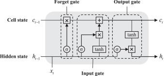
Fig. 2. Basic structure of an LSTM unit. |
2.2. Probabilistic forecasting
Assuming that is a set of sub-time series of wave elevation obtained from the raw experimental data using a fixed-length sliding window , where , is the wave elevation of the -th sub-time series sampled at time and denotes the total number of the sub-time series. It’s worth mentioning that the interval between any two adjacent time points is constant, defined by the wave sampling frequency. And each sub-time series consists of the past and future wave elevations, which are expressed separately as and .
Salinas et al. [23], Sprangers et al. [30] improved the performance of the model by incorporating several time-dependent and time-independent covariates. However, it remains unclear whether adding these covariates will improve the predictive performance for wave elevation time series. As a result, we aim to estimate the probability distribution of future wave elevation based on either wave elevation data or a combination of wave elevation data and covariates. The conditional distributions can be formulated as follows:
where signifies the first point in the future and denotes the covariate associated with wave elevation. The mean value and standard deviation parameterized by are the probability distribution parameters of the wave elevation at each forecasting time point . indicates the learnable parameters of the model, and all sub-time series share the same .
2.3. Architecture
Stack and Sequence to Sequence (S2S) are the two common frameworks used in constructing the RNNs [31]. Considering that the S2S architecture is better suited for long-time series prediction problems, all cases presented in this paper will utilize the S2S architecture to establish the mapping relationship between the past and future data, as illustrated in Fig. 1.
S2S is composed of two components: encoder and decoder. In the encoder network, the input features (e.g., wave elevation or covariate) are encoded at each time step, and then the encoded information is propagated along the RNN. As the encoded information propagates across the encoder network, the RNN continuously screens valuable information from the encoded information until the encoded information is delivered to the last LSTM unit. The output of the encoder network is used as the initial state of the decoder network to anticipate the future wave elevation by sampling through Equations (7) and (8). A distinguishing feature of the decoder network is that it generates multi-step forecasts via a recursive strategy. The prediction generated using the historical data is directly passed into the next LSTM unit as input. Through the use of a recurrent function , a multi-layer RNN with learnable parameters computes the hidden state . The dimension of is a critical hyperparameter that affects the model’s performance, and we will discuss how to determine in Section 3.5. Additionally, the of the current time step will be used as the initial condition for the next time step:
In the absence of covariates, then will be written as:
For each LSTM unit in the future horizon, the output is a two-dimensional array consisting of the mean and standard deviation . The dimension of the may differ from that of the predicted results, so we add a fully connected layer (FC) after the RNN to ensure that the dimension of the output is equal to 2:
Notably, to avoid scenarios where the standard deviation is less than or equal to 0, the anticipated standard deviation will be affinely transformed using a softplus activation function prior to output:
2.4. Likelihood model
As the likelihood function will influence the accuracy of the model, an appropriate likelihood function should be determined based on the statistical characteristics of the physical quantities to be predicted [23], [30]. For example, we can employ Gaussian (Fig. 3) or Student likelihood for real-valued quantities and Bernoulli likelihood for binary data. The wave elevations are generally considered to follow the Gaussian distribution. According to a statistical analysis of the wave elevation time series for sea state WC04 (shown in Fig. 5 (b)), it can be concluded that the statistical characteristics of wave elevation can be characterized by the Gaussian distribution. Therefore, we train the Deep-WP model using a Gaussian likelihood distribution as a fixed parameterized distribution. The probability density of the -th future wave elevation in the forecasting horizon can be formulated as follows:

Fig. 3. Probabilities for a Gaussian distribution, the percentage represents probability. |
2.5. Training
We trained and evaluated the model’s predictive ability using the open-source application Pytorch. In order to improve the training efficiency, the data set is again divided into multiple sub-datasets with the same size before training. Similar to the dimensionality of the hidden state of the LSTM unit, the size of the sub-dataset is a potential factor affecting the model’s performance. In Section 3.5, we will discuss how to set a reasonable mini-batch size in detail. The loss accumulated after each mini-batch sub-time series is trained back-propagates along the RNN to update the weight coefficients and biases of the LSTM unit. The loss is calculated via a negative log-likelihood function:
where is the -th ground truth in the sub-time series.
We will use adaptive momentum estimation (Adam) [32] to optimize the learnable parameters of the model. The maximum epoch size of training is set at 1000, i.e., one epoch represents one training for the entire sub-training set. If the validation loss does not decrease for 5 consecutive epochs, the learning rate will be reduced by a factor of 0.8. The overfitting problem is mitigated by early stopping criteria. If the model’s error on the validation set does not decrease for 20 epochs, then the training is stopped. Additionally, we will save 5 trained models with the lowest loss on the test set for predicting wave elevation.
The model configuration parameters are listed in Table 1.
Table 1. Network structure and training method used for the present model. |
| Deep-WP | |
|---|---|
| Number of LSTM layers | 3 |
| Dropout ratio | 0.1 |
| Number of FC layers | 1 |
| Affine function | Softplus |
| Likelihood model | Gaussian |
| Optimizer | Adam |
| Maximum epoch size | 1000 |
| Learning rate schedule | ReduceLROnPlateau |
| Early stopping | True |
| Number of best-trained models kept | 5 |
3. Numerical setup
3.1. Error metrics
The NDRMSE defined as Eq. (15) is essentially the root mean square error but normalized with the significant wave height to account for differences in different sea states:
where is the total number of points within the future horizon.
3.2. Datasets
We evaluate the ‘probabilistic’ forecasting performance of the Deep-WP model using the wave elevation trains generated in the deepwater offshore basin at Shanghai Jiao Tong University (SJTU), China. The basin is 50 m in length, 40 m in width, and 10 m in maximum effective depth. The artificial basin floor can be moved up and down to model various water depths within a range of 0–10 m in model scale. The waves can be generated on two adjacent sides of the basin by multi-flap wave makers. And two passive wave-absorbing beaches are located on the opposite sides of the wave makers.
Five irregular long-crested waves are generated following the JONSWAP spectrum (see Eq. (16)) with different significant wave height and peak period ,
where is the peak frequency, is the spectral peakedness parameters, and is the shape parameter ( if and if ). The scaling factor for this experiment is 1:64, and the and of the simulated waves are listed in Table 2.
Table 2. Wave parameters corresponding to the prototype and model. |
| Prototype | Model | |||
|---|---|---|---|---|
| Sea State | (m) | (s) | (m) | (s) |
| WC01 | 6 | 14.85 | 0.094 | 1.856 |
| WC02 | 8 | 14.85 | 0.125 | 1.856 |
| WC03 | 10 | 14.85 | 0.156 | 1.856 |
| WC04 | 12 | 14.85 | 0.188 | 1.856 |
| WC05 | 10 | 13.58 | 0.156 | 1.698 |
14 wave probes are arranged in the basin (as shown in Fig. 4) to measure the wave elevation. The sampling rate is 25Hz with a duration of 30 minutes (i.e., approximately 1000) in model scale. All wave elevation time series will be scaled up to prototype by a factor of 64 prior to constructing the training dataset. As the wave field is underdeveloped in the initial phase of the experiment, the first 3-min wave elevation time series are removed from the raw data. The training dataset with a duration of 4096s is randomly extracted from the measured wave surface elevations at a certain location. Then the dataset is divided into training set, validation set, and test set by the ratio of 0.8:0.1:0.1. It should be noted that the temporal nature of wave elevation should be considered during the dividing process [33]. Thus we will split the dataset into the training, validation, and test sets according to their temporal order of occurrence (as shown in Fig. 5 (a)). For example, if the dataset is 100s in length, the training, validation, and test sets would correspond to 1-80s, 81-90s, and 91-100s, respectively.

Fig. 4. Distribution of wave probes in the basin during the experiment (in model scale). |

Fig. 5. Wave elevation time series and probability density distribution for the sea state WC04 with m and s. |
3.3. Normalization
The normalization of the data prior to feeding it into the neural networks will speed up the convergence of the model. Given the randomness of waves, the statistical characteristics differ significantly between the sub-time series, we refer to the scaling mechanism from [23], [30] for normalizing the input data with a scale factor belonging to each sub-time series, and then scaling the model output to full scale by multiplying the scale factor:
3.4. Covariates

Fig. 6. The wave elevation at each time point and the corresponding covariates information. Using a wave elevation sub-time series with 6 points as an example, the absolute position P corresponds to the local position of wave elevation in the sub-time series, the timestamp refers to the moment in global time when wave elevation occurs, and the category W relates to the sea state to which wave elevation belongs. |
Table 3. Dimension of the covariates used in the Deep-WP model. |
| Covariate | Dimension |
|---|---|
| Absolute Position | 20 |
| Timestamp | 3 |
| Category | 20 |
The absolute position is represented by a fixed position embedding proposed in [34]:
where denotes the absolute position of the wave elevation in the sub-time series, and () indicate the dimension of the covariate, will directly affect the similarity of the different position embeddings, referencing [35].
For each timestamp, we employ a learnable stamp embedding from [34] to depict the periodic nature of, e.g., millisecond-of-the-second, second-of-the-minute and minute-of-the-hour. As the moment corresponding to each wave elevation sampling point was not recorded during the wave tank experiment, the timestamp for each wave elevation time series is assumed to be .
We utilize the learnable embedding [30] built into the PyTorch program to represent the category features. The category features correlate to wave category in the ocean wave forecasting datasets (e.g. 0 and 1 denote strong and weak nonlinear waves, respectively).
3.5. Hyperparameters
In addition to the neural network framework and wave dataset discussed above, the dimension of the hidden state, the initial learning rate, and the mini-batch size all influence the prediction accuracy. For simplicity, we test the effect of hyperparameters on prediction accuracy only with the wave elevation time series for sea state WC04. Since the length of the input also impacts the performance of the model, we create 8 different datasets by varying the lengths of the input within to predict 6 steps into the future. The hyperparameters are determined by performing a limited grid search using the following settings:
•Dimension : ,
•Learning rate : ,
•Mini-batch size : .
The result is shown in Fig. 7. We use the mean of the model’s NDRMSE over the 8 datasets as the selection criterion for the hyperparameters because each input length has the potential to minimize the NDRMSE of the model. When the hyperparameters are , the average NDRMSE of the model is the smallest (0.013). However, it takes approximately 218.961 seconds to obtain the local optimal solution. Considering the time cost and accuracy, the hyperparameters are determined as with the NDRMSE of 0.014. Though this NDRMSE is 0.001 greater than the minimum value, the model takes only 193.936 seconds to converge.
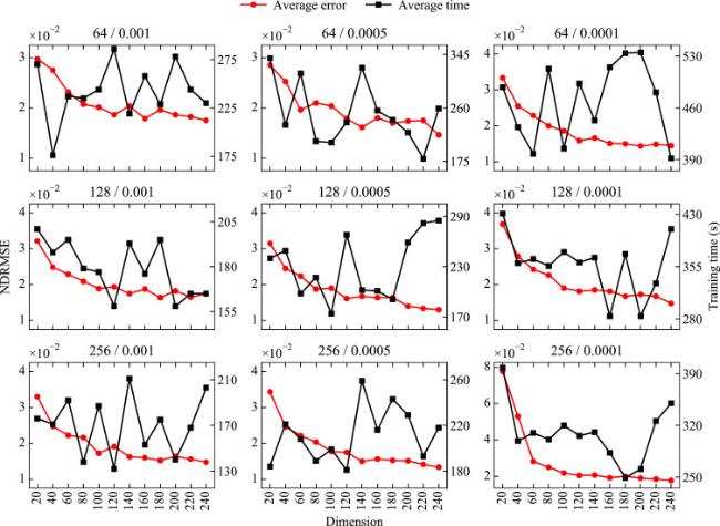
Fig. 7. The NDRMSE and training time for each mini-batch size and learning rate under different dimension of the hidden state for the sea state WC04. |
The framework is run on a PC equipped with an AMD Ryzen 9 5950X 16-Core CPU (3.8 GHz) and an Nvidia GeForce RTX-3070Ti 8GB GPU. The source code for this paper, as well as the wave elevation datasets, are accessible at https://github.com/liuhahayue/Deep-WP.
4. Results and discussion
4.1. The precision of the deep-WP model for different prediction ranges under single variable conditions
The Deep-WP model utilizes a recursive algorithm to predict the future wave elevation, and the accumulated error will directly impact the model’s performance over the entire prediction range [31]. Accordingly, we only evaluate the model’s performance for short periods of time. Considering that the sampling interval of wave elevation is 0.32s, and the for most of the sea states is 14.85s (about 47 time points) in full scale, we will predict the wave elevation at the next time points, which correspond to the duration of , respectively. In this example, only the historical wave elevation was fed into the Deep-WP model to forecast future wave elevation.
For each short-period prediction, we construct 8 datasets with variable input lengths by adjusting the ratio of inputs to outputs from 1 to 8. The Backpropagation Through Time algorithm is used to update the coefficients of the learnable parameters. Fig. 8 illustrates the NDRMSE distribution of the model on the test set for different sea states and prediction ranges. Notably, when the predicted number of points is 6 and 8, using the wave elevation information of the first 24 or 48 points may enable the model to achieve the minimum error. In the case of the prediction range is , although the increase in input data will help reduce error in most test cases, it also results in a significant increase in training time. Making trade-offs between the training efficiency and the prediction accuracy, the wave elevation information for the first 96 points is chosen as the input of the model.

Fig. 8. Statistical boxplots of NDRMSE on the test dataset for sea states WC01-WC05 with different forecasting horizons . |
Table 2 lists the parameters of 5 sea states. The sea states WC01-WC04 can be regarded as a same class of waves since they have the same wave characteristic parameters except for . The nonlinearity of sea state WC04 is obviously stronger than that of sea states WC01-WC03. As stated in Section 3.5, we determined the hyperparameters using the wave elevation time series for sea state WC04, thus the model is capable to capture strong nonlinear wave properties. As shown in Fig. 8, the NDRMSE of the model is smaller for sea states WC01-WC03 than for sea state WC04. This indicates that the hyperparameters determined by the strong nonlinear wave fields are also applicable to a weak nonlinear sea state with the same wave characteristics, simplifying the complex and time-consuming process of reassigning hyperparameters for different sea states. Furthermore, the of sea state WC05 is the same as that of sea state WC03, while the is different. Comparing the NDRMSE for sea states WC03-WC05, we find that although the prediction error of sea state WC05 is slightly higher than that of sea state WC03, it is comparable to that of sea state WC04. Referring to Eq. (16), it is clear that affects the shape of the wave spectrum more than , leading to a shift in the wave composition. In order to improve the accuracy of the model, we recommend that the hyperparameters should be selected based on the wave elevation time series corresponding to a certain .
Fig. 11, using the ‘probabilistic’ strategy, the Deep-WP model can increase the accuracy of its predictions by providing the confidence interval (CI) expressed as .

Fig. 11. Predicted wave elevation and confidence interval for the sea state WC04 on the test data set with different forecasting horizons . The prediction at each point is the mean (), whereas the shaded areas (red, blue, and green) correspond to confidence intervals of standard deviations (1, 2, and 3). For each subplot title, the integer represents the identifier of sub-time series in the test set. (For interpretation of the references to colour in this figure legend, the reader is referred to the web version of this article.) |
4.2. Effect of covariate information on the precision
Covariates are capable of improving the model’s performance when predicting seasonal and trend data [23], [30]. Since the ocean waves are extremely stochastic, it is debatable whether the introduction of covariates can improve the accuracy of such data as waves. The effects of covariate information on the performance of the Deep-WP model will be systematically investigated in this section.
To identify the suitable covariates for wave prediction, we will create five datasets based on different combinations of covariates and wave elevation: Elevation, Position, Category, Timestamp, and Global. Elevation only includes wave surface elevation; Position, Category, and Timestamp not only contain the wave elevation data but also introduce the absolute position, category, and timestamp information, respectively; and Global is all covariates combined with wave elevation at the same time. Table 4 lists the information contained in the different datasets.
Table 4. Input data for the current model. |
| Dataset | Information |
|---|---|
| Elevation | elevation |
| Position | elevation + absolute position |
| Category | elevation + category |
| Timestamp | elevation + timestamp |
| Global | elevation + absolute position + category + timestamp |
Table 5 summarizes the NDRMSE of the model under various covariates for sea states WC01-WC05. This error is calculated in the same manner as hyperparameter selection. All three covariates employed in the experiment contribute to reducing the prediction error, with the absolute position information providing the best prediction outcome. Though the LSTM unit can capture the temporal relationships in the wave elevation time series, the absolute position information can directly inform the model about the absolute position of each time point in the sub-time series. The weak periodicity of the wave makes the discrepancies between sub-time series of neighboring , resulting in slightly lower precision of timestamps than absolute position. Generally, the introduction of category information increases the prediction error substantially, especially for wave fields with strong nonlinearity, such as sea states WC03-WC05. As for the effect of global information on the model performance, it gives similar accuracy to absolute position information with a predicted target number of points is 24 or 48, except for sea state WC04.
Table 5. The NDRMSE of the Deep-WP model under different covariates and prediction lengths for sea states WC01-WC05. Lower is better, the best-performing dataset is highlighted in bold. The count is the total number of prediction errors that contain covariates that are lower than or equal to the prediction errors using elevation alone for different prediction lengths. |
| Metric | NDRMSE | |||||
|---|---|---|---|---|---|---|
| Length | 6 | 8 | 12 | 24 | 48 | |
| WC01 | Elevation | 0.018 | 0.032 | 0.063 | 0.144 | 0.209 |
| Position | 0.019 | 0.031 | 0.062 | 0.123 | 0.189 | |
| Category | 0.020 | 0.040 | 0.068 | 0.144 | 0.198 | |
| Timestamp | 0.019 | 0.028 | 0.067 | 0.139 | 0.199 | |
| Global | 0.020 | 0.033 | 0.064 | 0.134 | 0.190 | |
| WC02 | Elevation | 0.014 | 0.021 | 0.043 | 0.093 | 0.156 |
| Position | 0.013 | 0.021 | 0.038 | 0.093 | 0.154 | |
| Category | 0.015 | 0.023 | 0.052 | 0.101 | 0.162 | |
| Timestamp | 0.013 | 0.022 | 0.045 | 0.101 | 0.161 | |
| Global | 0.016 | 0.024 | 0.044 | 0.088 | 0.155 | |
| WC03 | Elevation | 0.011 | 0.018 | 0.033 | 0.089 | 0.137 |
| Position | 0.011 | 0.016 | 0.031 | 0.076 | 0.146 | |
| Category | 0.013 | 0.021 | 0.037 | 0.102 | 0.169 | |
| Timestamp | 0.010 | 0.016 | 0.034 | 0.074 | 0.153 | |
| Global | 0.013 | 0.019 | 0.032 | 0.081 | 0.140 | |
| WC04 | Elevation | 0.014 | 0.025 | 0.048 | 0.097 | 0.164 |
| Position | 0.016 | 0.022 | 0.041 | 0.099 | 0.159 | |
| Category | 0.017 | 0.024 | 0.053 | 0.120 | 0.172 | |
| Timestamp | 0.014 | 0.024 | 0.044 | 0.102 | 0.169 | |
| Global | 0.015 | 0.021 | 0.043 | 0.098 | 0.169 | |
| WC05 | Elevation | 0.018 | 0.027 | 0.064 | 0.139 | 0.179 |
| Position | 0.016 | 0.029 | 0.064 | 0.129 | 0.172 | |
| Category | 0.018 | 0.031 | 0.074 | 0.140 | 0.181 | |
| Timestamp | 0.017 | 0.030 | 0.068 | 0.141 | 0.175 | |
| Global | 0.019 | 0.031 | 0.063 | 0.131 | 0.171 | |
| Count | 8 | 9 | 9 | 11 | 10 | |
Training efficiency is another important factor to measure model performance. The training time and NDRMSE for the five different types of datasets are normalized using Elevation as the baseline. Fig. 12 demonstrates the effect of covariates on the performance of the Deep-WP model. In general, covariates are employed to assist in predicting, and the model needs to be trained for longer periods of time to converge. Notably, the training time of the Deep-WP model does not increase exponentially and still retains a high training efficiency. We recommend that the absolute position or the timestamp should be combined with the wave elevation to enhance the model’s performance.

Fig. 12. Training time compared to NDRMSE on the test set for sea states WC01-WC05 under different covariates and prediction lengths, where Elevation is the baseline. |
4.3. Model applicability to waves with different energy components
In marine engineering applications, the wave signals gathered by probes are contaminated by a variety of noises. They must be filtered to satisfy the needs of practical application scenarios. The nonlinear random waves can be viewed as a superposition of sinusoidal waves of unequal amplitude, with the frequency of each wave component directly determining its amplitude, according to Eq. (20):
where denotes the random phase of the -th wave component, and .
In this example, the original wave elevation data for sea state WC04 will be filtered by 1.5, 2.0, 2.5, 3.0, and 4.5 times (), respectively. The filtered wave elevation time series will be utilized to train and evaluate the Deep-WP model. The hyperparameters and architectures of the current model are determined by the case with a filtering frequency of . As illustrated in Fig. 13, there exist significant discrepancies between the wavelet peaks of the wave elevation time series following different filtering frequencies. The energy ratio of the filtered waves relative to the original data is presented in Table 6.
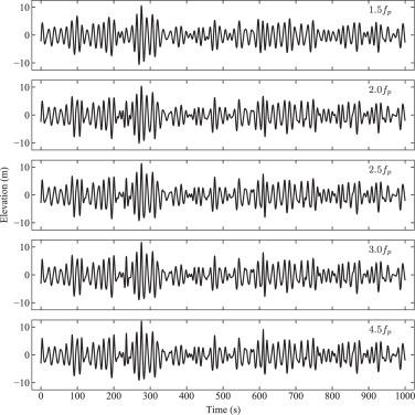
Fig. 13. The wave elevation time series generated by the different filter frequencies for sea state WC04. In order to display the differences in waves after filtering at different frequencies, only a portion of the wave time series (approximately 1000s) is depicted in the figure, and the time duration of the wave time series corresponding to each filtering frequency during training is 4096s. |
Table 6. Remaining energy after wave filtration. |
| Frequency | Energy ratio (%) |
|---|---|
| 1.5 | 76.055 |
| 2.0 | 89.324 |
| 2.5 | 94.642 |
| 3.0 | 97.059 |
| 4.5 | 99.419 |
The NDRMSE with different filtering frequencies are shown in Fig. 14. After the original wave elevation time series are filtered by 1.5 or 2.0 times , the newly generated wave elevations have weaker nonlinearity, and the error is lower than . In particular, the model’s accuracy is highest when the filtering frequency is . In the case of , the filtered wave has approximately 97.059% of the energy of the unfiltered wave. The error increases slightly, indicating that the Deep-WP model can be extended to wave fields with strong nonlinearity. When the predicted waves have almost no energy loss (), the model is no longer appropriate for short time series prediction, but its accuracy for long time series prediction remains good. Given that the Deep-WP model has the potential to capture the time-domain characteristics of the strongly nonlinear wave field, the hyperparameters should be redefined based on the wave elevation time series corresponding to .

Fig. 14. The Deep-WP model’s prediction error on the test set with different filtering frequencies and different covariates for different prediction lengths . The E, P, C, T, and G correspondingly represent Elevation, Position, Category, Timestamp, and Global. |
Furthermore, as the length of the prediction and the energy contained in the wave field increase, we observe that the covariates significantly reduce the models error. This is yet another demonstration of the validity of covariates for wavefield prediction.
5. Conclusions
In this study, we attempt to forecast the measured wave data by the Deep-WP model based on a ‘probabilistic’ strategy. It is shown that the ‘probabilistic’ strategy can be utilized to predict short term wave time series with excellent accuracy, particularly with a prediction length of points. Three kinds of covariates are introduced to assist in prediction. When the wave elevation information is paired with absolute position or timestamp, the model enhances accuracy without losing training efficiency. Moreover, the generalization of the model with wave elevation time series containing different energy components is tested. The hyperparameters determined by wave fields with a strong nonlinearity also applies to wave fields with weak or slightly stronger nonlinearity.
Since our objective is to verify the applicability of the ‘probabilistic’ strategy for real-time wave prediction, we only optimize some model’s hyperparameters, including the dimension of the hidden state, the learning rate, and the mini-batch size. The model’s outcomes are also influenced by the hyperparameters related to the structure [30], [31] (e.g., the number of hidden or fully connected layers). In addition, the Deep-WP model must be retrained for each sea state to maintain a high level of forecast precision. If numerous different sea states are predicted simultaneously, it will add additional training costs. In later work, we will further optimize the Deep-WP model to make it capable of predicting numerous sea states at the same time.
Declaration of Competing Interest
The authors declare that they have no known competing financial interests or personal relationships that could have appeared to influence the work reported in this paper.
Acknowledgement
This work is supported by Hainan Provincial Natural Science Foundation of China (Grant no.520QN290), the 2020 Research Program of Sanya Yazhou Bay Science and Technology City (Grant No. SKJC-2020-01-006) and the Hainan Provincial Science and Technology Plan-Sanya Yazhou Bay Science and Technology City Natural Science Foundation Joint Project (2021JJLH0062).
Supplementary materials
Supplementary material associated with this article can be found, in the online version, at 10.1016/j.joes.2022.08.002
