
1. Introduction
A Tension Leg Platform (TLP) is a hybrid, compliant platform moored by tendons that connect the structure and anchor on the sea bottom. Its position is maintained by tendon tension created by excess buoyancy of the floating structure, and therefore, it is stabilized by tendon tension and platform buoyancy. It is designed to sustain springing and ringing responses that are correlated with short-period motion [27], [28], [29]. TLP has six degrees of freedom (DOF) motion, where its roll ξ4, pitch ξ5 and heave ξ3 are short-period motions that are different from surge ξ1, sway ξ2, and yaw ξ6 that are long-period motions. To avoid first-order wave excitation, the period of short-period motion should be far from the wave period in the region of wave energy concentration. The heave, roll, and pitch natural periods should be shorter than 3.5 s, and the surge and sway natural periods should be longer than 25 s. Otherwise, resonance, a sensitive motion, can be easily obtained [2,11,24,38,39]. The difference in the natural period between horizontal motion and rotation is so great that analysis of horizontal motion and decoupled rotation can be performed; therefore, this study decouples roll motion from the motion of the other five degrees of freedom. Waves flow onto the TLP deck and then become green water. Green water is a very complex physical phenomenon. It is a sensitive motion that is strongly nonlinear, so that it is difficult to model by mathematical theory. TLP's sensitive motions of resonance and green water are affected by roll, pitch, and heave. Thus, it is better to intervene and control the roll, pitch, and heave of a TLP before sensitive motions occur. Therefore, this study develops a precontrol methodology to restrict sensitive short-period motion.
Precontrol is not a general control approach, and its core idea is to take corrective measures in advance before the occurrence of sensitive motion. Generally, the control approaches include active control and passive control, and they are divided by energy input types. Active control needs energy input, such as for the adjustment of the TLP tendon length by a computer-controlled hydraulic system according to the sea state and working conditions; passive control does not need energy input, such as for the use of helical strakes attached to the surface of a pontoon and buoyancy modules attached to risers to passively control the turbulence of vortex-induced vibration of cylindrical structures [4]. Active control and passive control are real-time control technologies that take measures to intervene after the occurrence of sensitive motion. This may cause damage if the control measures are not sufficiently strong. Unlike active and passive control, precontrol [17] is a "preventive" method that takes measures to intervene before sensitive motion occurs.
Short-period motion, such as roll motion, directly affects the safety of TLPs. Therefore, a reliable prediction model is important for ensuring safety [30,33,43]. Previous work by Virgin [34] used a numerical and phenomenological approach to analyse roll motion using a semiempirical nonlinear differential equation, and Soliman presented both steady and transient analyses of the semiempirical nonlinear differential equation [26]. The horizontal motion of the TLPs is mainly due to the drift force that includes the contributions of the viscosity force, drag force, and second-order drift force. Slow-drift and sum-frequency forces may play a role in tendon loading, but TLP mooring loads are primarily linked to first-order wave loads [2,6,29]. The second-order wave loads enhance roll motion [40]. Researchers have conducted investigations of roll motion from the aspects of safe basins and heteroclinic orbits [7,16,31,32]. A statistical methodology has been extended to the nonlinear capsize problem in random sea waves with multiple degrees of freedom. The study of transient motions and the erosion of a safe basin mapped in the space of initial conditions leads to significantly less conservative and potentially more accurate predictions of ultimate dynamic stability [10,15,[18], [19], [20],36,42].
Model tests find that the occurrence of green water and loading depends strongly on wave steepness and current velocity. Green water cannot be predicted accurately with the present methods based on linear wave theory [5]. Green water is related to the vertical relative motion with respect to the wave surface, and the probability of green water is related to the threshold of vertical relative motion exceeding the freeboard [8,9]; therefore, roll and heave motions affect green water. In theoretical analysis, potential flow theory, wave overtopping theory, flood wave theory, and probabilistic methods are general approaches to solving the green water problem [8,25,45]. In numerical simulations, a nonlinear dynamic, implicit time-stepping procedure and a 3-D numerical wave tank with the dynamic mesh technique are applied to simulate green water [14,25,44]. Experiments are some of the most effective approaches to solving the green water problem. Experimental research shows that the maximum fluid particle velocity, as well as the bubble velocity in front of the structure during the impingement process, is approximately 1.5 times greater than the phase speed of the waves. The maximum horizontal velocity above the deck is lower than the phase speed. In the deck-impingement case, the maximum horizontal velocity is higher for the case with waves compacting on the deck, and waves also pass the deck much faster. The profiles of the green water velocity show a nonlinear distribution, with the maximum velocity occurring near the front of the water [1,[21], [22], [23].
The technologies that solve TLP's sensitive short-period motion are too complicated to apply in practice. Therefore, an effective and simple methodology is needed. This paper develops a precontrol methodology to prevent the occurrence of sensitive motion in advance by applying a constraint regime based on a series of simple and high-fidelity numerical models for short-period motion. Based on the numerical models and the range of sensitive short-period motion, a constraint regime developed by the multilevel parameter constraint domain is generated. The constraint regime consists of two parts: the control range (corresponding to sensitive short-period motion) and the opposite feasible range. Changing the control from a remedial action to a preventive action is the advantage of precontrol methodology that goes beyond the conventional wisdom of real-time control. The disadvantage of this methodology lies in the analysis of the control stability in the system design phase that increases the complexity of the design process. The basic organization of this article is as follows: in Section 2, the precontrol methodology of TLP's short-period motion is presented. In Section 3, multilevel precontrol of the TLP's short-period motion is given to build the foundation of the constraint regime. In Section 4, the precontrol and constraint regimes of the TLP's short-period motion are discussed. Finally, the conclusions of this work are given in Section 5.
2. Precontrol methodology of TLP's short-period motion
2.1. Precontrol-constrained regime mapping relationship
Precontrol takes action before the occurrence of a phenomenon, and it is achieved by the constraint regime, which is a preimage in the precontrol-constraint regime logical relationship. The objective of precontrol is an image (objective performance), corresponding to that preimage (parameter-domain) by the function mapping relationship (parameter-performance numerical models).
It is more advantageous to fully consider sensitive motion regions that need to be avoided at the time of scheme design. Sensitive motion regions deduce the boundary of the main parameters to generate the parameter constraint domain by applying function mapping relationships with parameter-performance numerical models. The dominant parameters should be fully constrained, and the nonsignificant parameters should be fully unconstrained. The parameter constraint domain is generated by focusing on the main contradiction and aiming at the core target to reduce the complexity of body design due to the coupling effect between various parameters. The design is carried out within the parameter constraint domain so that the designed body has a good motion performance that meets the design requirements. This design eliminates the need for active or passive control remedies after the occurrence of sensitive motions. The set of all parameter constraint domains is the constraint regime.
The objective of precontrol (image)—parameter-performance numerical models (function mapping)—constraint regime (preimage) is the body performance that meets the design requirements (image) forms the logical mapping relationship of precontrol. Furthermore, this is a closed control logic (Fig. 1).
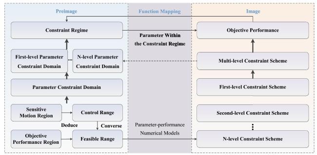
Fig.1 The logical chain of precontrol. |
Generally, the objective of precontrol is decomposed into a multilevel constraint scheme according to multilevel function mapping. The constraint scheme is established as a multilevel constraint in the logical order of importance. The one-level constraint localizes the parameter's scope, and the multilevel constraint localizes the parameter's scope level by level to achieve the narrow band of parameters. The parameter constraint domain of the previous level is the input of the next level. Finally, the multilevel parameter constraint domains are assembled into the entire constraint regime. This constraint regime achieves precontrol by applying a multilevel parameter-in-constraint domain.
2.2. Precontrol procedure of TLP's short-period motion
The precontrol of the TLP's short-period motion is decomposed into a two-level constraint. The first is the natural period of roll and heave constraint, and the other is the green water constraint. According to the severity of threats of sensitive motion, the natural period of roll and heave constraint is defined as the primary objective, and the green water constraint is defined as the secondary objective. The parameter constraint domain of the natural period of roll and heave is the input of the green water constraint. A two-level parameter constraint domain is used to investigate the constraint regime to achieve precontrol of the TLP's short-period motion (Fig. 2).
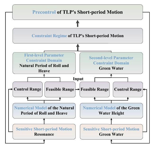
Fig.2 Workflow of precontrol of TLP's short-period motion. |
3. Multilevel precontrol of TLP's short-period motion
This section demonstrates the feasibility of precontrol of short-period motion by applying a parameter constraint domain based on the parameter-performance numerical models. This study develops (1) the natural period of the roll and heave model and (2) the green water height model as parameter-performance numerical models.
3.1. First-level precontrol based on the natural period of roll and heave model
The natural periods of roll and heave are generally less than 4 s. These characteristics of the short period overlap with the wave period of the wave energy concentration region, inducing resonance. Therefore, restricting the natural period of roll and heave to avoid the wave energy concentration region is important. Constraint of the natural period of roll and heave involves two important steps: development of the numerical models of the natural period of roll and heave and analysis of the influence laws of the TLP's parameters on the natural period.
3.1.1. Model of roll motion
(1) Mathematical Model of Roll Motion
TLP roll motion decoupled from the motion of the other five degrees of freedom is modelled using a semiempirical nonlinear differential equation. The following nonlinear differential equation is the general form of the governing equation of roll motion forced by external excitation, such as waves and wind:
where θ is roll angle, rad;
I44 is the roll moment of inertia, kg·m2; A44 is the added mass of roll motion, kg·m2;
b1, b2, c1, c2, c3, c4, c5 are coefficients, where b1 is the first-order damping coefficient, b2 is the second-order damping coefficient, c1 is the first-order stiffness coefficient, c2 is the second-order stiffness coefficient, c3 is the third-order stiffness coefficient, c4 is the fourth-order stiffness coefficient, and c5 is the fifth-order stiffness coefficient;
Mwave( t) is the wave disturbance torque, N·m; Mflow( t) is the flow disturbance torque, N·m; and Mwind( t) is the wind heeling moment, N·m.
This governing equation is difficult to apply in simulations because many frequency-dependent hydrodynamic coefficients are needed. The simplified model introduced below makes it much easier to simulate the roll motion.
(2) Simplified Model of Roll Motion
TLP moves with six degrees of freedom when forced by buoyancy, gravity, tendon pretension and wave loads (Fig. 3). TLP's excessive buoyancy due to tendons connecting the structure and anchors on the sea bottom is proportional to the draft. The parts of the submerged floating structure are semisubmerged corner columns and fully submerged pontoons, which are regular structures. Because draft variation is proportional to heave displacement, it is appropriate to use Spring k to represent the constitutive relationship of the TLP's buoyancy (Fig. 4). Increasing draft leads to a buoyancy increase that represents a pretension increase and vice versa. Tendons are assumed to have a linear constitutive relation, so that pretension is proportional to their tensile displacement. TLP is designed to retain excessive buoyancy, which in turn is compromised by variable submergence effects in heave motion. In the equilibrium position, initial buoyancy and initial pretension offset each other; tension variation, which offsets gravity and initial buoyancy, is proportional to heave displacement with the motion starting from the equilibrium position. Therefore, the use of Spring k1 to represent the constitutive relationship of tendons is appropriate (Fig. 4). An increase in the draft is associated with an increase in net buoyancy and/or a reduction in pretension to a certain degree. The differences in tendon length when the TLP moves can be ignored because the length variation of tendons is small compared to the initial length. TLP is approximately horizontally symmetric, and its four tendons form two groups due to roll motion pivoted on an axis. Each group has the same tensile displacements on the same side of the heel, leading to the same roll angles for each group in roll motion.
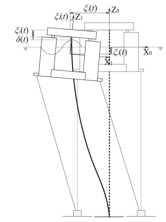
Fig.3 Simplified model of TLP roll motion. |
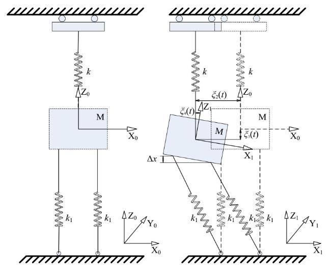
Fig.4 Simplified model of roll motion. |
In this study, the TLP's floating structure is modelled by a mass M, and tendons are modelled by two springs k1 that are equivalent to the constitutive relation coefficient. TLP's buoyancy is modelled by Spring k that is equivalent to the waterplane area coefficient. This simplified model is appropriate to analyse the kinematics and dynamics of roll motion (Fig. 4).
Following the simplified model of roll motion, a numerical model is established to investigate the natural period of roll motion based on stability theory. The core concept of this numerical model for the natural period of roll motion is as follows: any roll angle is a potential rolling critical point in the first ¼ cycle of roll motion. A rolling critical point may be either a stable centre point or an unstable saddle point. Based on stability theory, within one cycle of roll motion, if a rolling critical point is a centre point, the roll motion is stable at this moment, and the body will continue to move to the next moment and position. If a rolling critical point is a saddle point, the roll motion is unstable at this moment, and the body cannot return to the equilibrium position in the future, indicating that the first ¼ cycle of roll motion has ended. The saddle point leads to the capsizing of the TLP, which is not true in normal operating conditions. Based on this stability analysis of roll motion, it is assumed that in a single period of roll motion, the time history corresponding to the condition of the last stable rolling critical point is a ¼ roll natural period. Based on this assumption, a MATLAB code was built to calculate every roll angle and determine the stability of every roll angle. The code simulates the time history corresponding to the condition of the last stable rolling critical point in a single period of roll motion and applies the time history to obtain the natural period of roll motion. The workflow of the calculation of the natural period of roll motion is as follows:
1. Establish the governing equation of roll motion.
2. Obtain critical points of roll motion and infer the stability of critical points.
3. Obtain the ultimate stable time of the critical point of roll motion.
4. The ultimate stable time of the critical point of roll motion is ¼ the natural cycle process. Based on this, calculate the natural period of roll motion.
3.1.2. Model of the natural period of roll motion
(1) Governing equation of roll motion and critical points calculation
Based on Eq. (1), considering the quadratic term of roll damping, roll motion is divided into three components: rotation and vertical and horizontal motion.
In the equations above, C is the roll damping coefficient, N·s2/rad2; k is the buoyancy coefficient, N/m; k1 is the spring constant of tendons, N/m; z is the heave displacement coupled with roll motion, m; x1 is the increment of tendons and is a function of time, m; t is time, s; δx is the length difference between the two groups of tendons caused by the roll motion in the roll plane, m; d is the horizontal distance of the two groups of tendons in the roll plane, m; L is the original length of the tendon, m; m is the TLP mass, kg; G = mg is the TLP weight, N; and δx is very small compared to the original length of the tendons, so that it can be ignored. Notably, this model does not include tether tension variations in the dynamic response. The roll angle θ is a function of time and can be obtained by solving the governing equation of roll motion. At every critical point, roll angular velocity is zero, and roll angular acceleration is a maximum. Let
Let f = 0, to solve for critical points.
The critical points equation is obtained as follows:
Because roll angle θ is a function of time, rolling critical points θc can be obtained by solving Eq. (6) as follows:
where a is the initial roll angle coefficient, corresponding linearly to the initial roll angle θinit, a is the dimensionless initial roll angle, and t is the time, s.
The initial roll angle coefficient a determines the TLP's initial roll condition (position and angular velocity). The initial roll condition affects the dynamic characteristics of roll motion, which in turn affects the natural period of roll motion. From the rolling critical points θc equation, it is known that roll angular acceleration is a constant. Consequently, the initial roll angle coefficient does not determine roll angular acceleration . At this point, critical points θc given by Eq. (7) are general solutions. To obtain a particular solution, an initial boundary condition is needed to determine the initial roll angle coefficient. Because any position can be the initial position before rolling, a specific value of the initial roll angle coefficient cannot be obtained. Because the initial roll angles should be less than 90°, it is obtained that a∈[-2.5066,2.5066].
(2) Inferring the stability of critical points of roll motion
Taking the derivative of f with respect to θ, we obtain
Eq. (7) for rolling critical points θc is applied to calculate the value of . If is greater than zero, the rolling critical point is a saddle point for which the motion trajectory is not cyclical, and the roll motion is unstable. If is less than zero, the rolling critical point is a centre point for which the motion trajectory is cyclical, and the roll motion is stable.
The value of is calculated for every roll angle to infer rolling stability. The results suggest that within a limited period, as time progresses, oscillates between negative and positive. This phenomenon indicates that the rolling critical points θc oscillates between stable and unstable. Based on the core concept of the spring-mass system, it is evident that the time history corresponding to the condition of the last stable rolling critical point is a 1/4 natural cycle process when the roll motion is within one cycle.
This study uses the LH16-2 TLP project as an example (Fig. 5). In this case, the TLP weights and loads are approximately 43,188 t.

Fig.5 The configuration of the TLP. |
The results of the numerical simulations of the time history of rolling critical points are shown in Fig. 6 (fixed z as a constant, set a free) and Fig. 7 (fixed a as a constant, set z free).
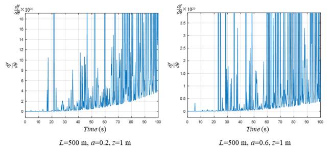
Fig.6 Numerical simulation of the time history of parametric rolling critical points ( L=500 m, z=1 m). |
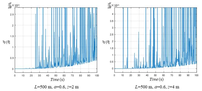
Fig.7 Numerical simulation of the time history of parametric rolling critical points ( L=500 m, a=0.6). |
For the numerical simulation shown in Figs. 6 and 7, within a limited period, as time progresses, oscillates between negative and positive. This phenomenon indicates that the rolling critical points θc oscillates between the centre point and saddle point, and the condition of the rolling critical points θc oscillates between stable and unstable. Under this condition, the TLP cannot cyclically roll in the upright equilibrium position. Roll trajectories vary with different levels of external disturbance. In the initial phase of roll motion, is negative and approximately zero. This shows that the TLP is in a stable state with a small external disturbance. The roll state is determined by the external disturbance after the initial phase of roll motion. After the initial phase with a small external disturbance, as roll motion progresses over time, oscillates between negative and positive. This indicates that the rolling critical points θc oscillates between the centre point and saddle point, and the rolling critical points θc oscillates between the stable condition and unstable condition. TLP may reach an equilibrium at different positions. However, these positions are not in upright equilibrium. After a period progresses, the value of for most operating conditions is greater than zero. These critical points are saddle points, corresponding to unstable roll motion. In some states, these saddle points and unstable roll motion may lead to dangerous situations. The roll motion is so complex that its trajectories depend on the initial condition, boundary condition and governing equation.
(3) Natural period of roll motion
In the motion of the spring-mass system with only one degree of freedom, if the mass moves to a terminal point, the restoring force of the spring is greatest. In time history, when the acceleration of a mass is either at a global extremum or a local extremum, the velocity of the mass is equal to zero, and its displacement is maximum. Within a single cycle process of roll motion, when roll angular acceleration is either at a global extremum or a local extremum, roll angular velocity is minimum and is equal to zero, and roll angle and roll amplitude are maximum. This time history is a 1/4 cycle process of roll motion that corresponds to 1/4 natural period of roll motion. In the time history obtained by numerical simulation of parametric rolling critical points, when reaches the last negative point in the time history, this condition indicates that roll motion reaches the final stable point that can be used as a 1/4 natural period of roll motion. This is used in the present work to obtain a natural period of roll motion. The natural period of roll motion Tnr is given by:
where Tnr is the natural period of roll motion, s, and tqr is the time corresponding to the last negative critical point in the numerical simulation of the time history of critical points, s.
(4) Example Study
Two experimental studies reported in the literature are used to validate the high fidelity of this simple numerical model of the natural period of roll motion. More details about these studies can be found in their paper.
(1) A MOSES TLP
The details of the prototype and model of the MOSES TLP are listed in Table 1, and the experimental setup information is shown in Figs. 8, 9. The MOSES TLP is analysed with a coupled dynamic response, and its experimental data on the RAO of roll motion are shown in Fig. 10.
Table 1 MOSES TLP prototype and model data [13]. |
| Parameter | Prototype | Model |
|---|---|---|
| Displacement (△) | 6779 t | 38.6 kg |
| Mass (M) | 5022 t | 28.6 kg |
| Diameter of hull | 22.4 m | 400 mm |
| Diameter of columns | 3.5 m | 63 mm |
| Length of tether (Lt) | 202 m | 3.6 m |
| Total tether stiffness (4EA/Lt) | 6.43 × 10⁸ N/m | 205.14 × 10³ N/m |
| Natural period of roll | 1.21 s |
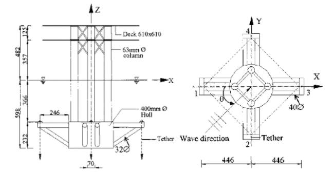
Fig.8 Geometric details of the MOSES TLP [13]. |
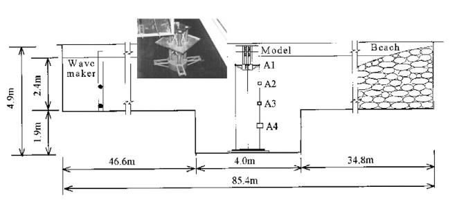
Fig.9 Experimental setup for the MOSES TLP [13]. |
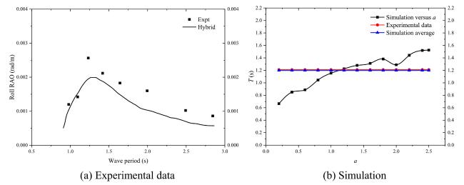
Fig.10 Comparison of the simulation and experiment for the MOSES TLP. |
The experimental data show that the natural period of roll motion is 1.21 s. The numerical model proposed by this study is applied to investigate the natural period of roll motion of the MOSES TLP. The results show that the natural period of roll motion increases with increasing initial roll angle coefficient, and the average natural period of roll motion is almost equal to the experimental results (Fig. 10).
(2) A SeaStar TLP
The details of the prototype and model of the SeaStar TLP are given in Fig. 11 and Table 2.
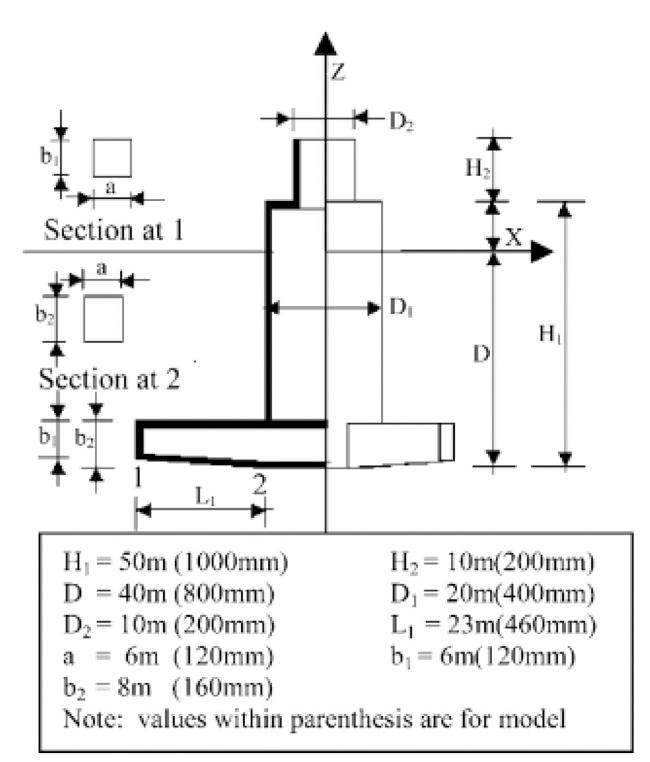
Fig.11 Geometric details [3]. |
Table 2 SeaStar TLP prototype and model data [3]. |
| Parameter | Prototype SeaStar 'A' | Model of SeaStar 'A' |
|---|---|---|
| Displacement | 15460 t | 124 kg |
| Mass | 11460 t | 92 kg |
| Length of tether | 175 m | 3.5 m |
| Diameter of columns | 20 m | 400 mm |
| Stress of tethers | 152.73 N/mm2 | 28.37 N/mm2 |
| EA | 1.8333 × 10¹⁰ N | 176750 N |
| Roll natural period | 1.58 s | 1.58 s |
The experimental data show that the natural period of roll motion is 1.58 s. The numerical model proposed by this study is applied to investigate the natural period of roll motion of the SeaStar TLP. The results show that the obtained values of the average natural period of roll motion are almost equal to the experimental values (Fig. 12).
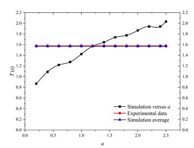
Fig.12 Comparison of the simulation and experiment of the SeaStar TLP. |
Comparison to the experimental results for two TLPs indicates that the numerical model of the natural period of roll motion proposed by this study is successfully validated by the experimental data. This numerical model can reliably calculate the natural period of roll motion when limited platform information is available and the natural period of roll motion must be estimated rapidly.
3.1.3. Sensitivity analysis of principal parameters for the natural period of roll motion
Here, the natural period curves are plotted versus as the TLP principal parameters to show the effects of the parameters on the natural period of roll motion. The principal parameters are weight and roll damping.
(1) Weight
The natural period of roll motion Tnr as a function of the TLP weight is shown in Fig. 13. Tnr increases with increasing initial roll angle coefficient a and is significantly impacted by weight. For 0< a<0.2, the initial roll angle θinit is very small, and Tnr increases with increasing a. In this branch, Tnr grows approximately linearly as a increases with a quite high growth rate. Weight has little influence on Tnr. For a>0.2, Tnr increases with increasing a, but the growth rate decreases and is lower than that in for 0< a<0.2. In this branch, weight has a great influence on Tnr. As weight increases, average Tnr decreases monotonically, and its slope decreases. Tnr curves for different weights cross. For a given constant weight, Tnr curves fluctuate as a increases. In this condition, Tnr is unsteady because it is perturbed by a. If a is kept constant, Tnr curves fluctuate with increasing weight; in this condition, Tnr is unsteady because it is perturbed by weight. The fluctuation of Tnr curves shows that Tnr changes with different a and weight values. This behaviour can effectively enable the system to avoid entering the overlapped domain of the TLP's natural frequency and ambient excitation frequency, leading to fewer occurrences of resonance. The influence of weight (inertia force) on the natural period of roll motion is not affected by the state of motion. Rather, it is an inherent property. The effect of unit weight W*=Δ/ mg (Δ displacement, mg weight) on Tnr is approximately 40%. Therefore, it is clear that weight has a significant impact on Tnr. Generally, low weight corresponds to greater Tnr; increasing weight decreases Tnr monotonically, and the slope decreases.
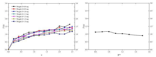
Fig.13 Effects of weight on the natural rolling period. |
The influence law states that the average natural period of roll motion is a decreasing function of the TLP weight, but there are some unstable disturbances (the natural period of roll motion increases as the TLP weight increases). In practice, the weight of a TLP can be modified by ballasting.
(2) Roll damping
The natural period of roll motion Tnr as a function of roll damping coefficient C is shown in Fig. 14. Tnr increases with increasing initial roll angle coefficient a and is significantly impacted by roll damping. For 0< a<0.2, the initial roll angle θinit is very small, and Tnr increases with increasing a. In this branch, Tnr grows approximately linearly as a increases with a quite high growth rate. Roll damping has little influence on Tnr. For a>0.2, Tnr increases with increasing a, but the growth rate decreases and is lower than that in for 0< a<0.2. In this branch, roll damping has a strong influence on Tnr. Generally, the average Tnr increases monotonically as roll damping increases. Under the condition of some roll damping, Tnr curves for different values of C cross. If roll damping is kept constant, Tnr curves fluctuate as a increases. Under this condition, Tnr is unsteady because it is perturbed by a. If a is kept constant, Tnr curves fluctuate as roll damping increases. Under this condition, Tnr is unsteady because it is perturbed by roll damping. The fluctuation of Tnr curves shows that Tnr transforms for different values of initial roll angle and roll damping. This attribute can be used to effectively avoid entering the overlapped domain of the TLP's natural frequency and ambient excitation frequency, leading to fewer occurrences of resonance for strong roll damping. The influence of damping (viscous force) on the natural period of roll motion is affected by the state of motion, and damping is one of the main factors of the damped natural frequency. The effect of unit roll damping C*=2 C/ ρD on Tnr is approximately 70%. Therefore, it is clear that roll damping has a significant impact on Tnr. Generally, lower damping has a smaller Tnr; increasing damping increases Tnr monotonically.

Fig.14 Effects of the roll damping coefficient C on the roll natural period. |
The influence law states that the natural period of roll motion is a monotonically increasing function of roll damping, but some oscillations are present. The roll damping coefficient can be determined by the theoretical solution of structural shape damping with potential theory or by numerical simulations.
Based on the above analysis, the initial roll angle θinit, weight and damping are sensitive factors for the natural period of roll motion Tnr. Tnr increases with increasing θinit, Tnr decreases with increasing weight, and Tnr increases with increasing damping. These sensitive parameters can be used to restrict the natural period of roll motion. The numerical model of the natural period of roll motion is verified by experiments, and its deduced numerical results are consistent with the laws of physics.
3.1.4. Model of the natural period of heave motion
Heave motion ξ3 is similar to roll motion ξ4, and its governing equation is defined as:
Based on linear theory, the natural period of heave motion is . The TLP weight, tendons and waterplane area coefficient can impact the natural period of heave motion.
3.1.5. Sensitivity analysis of the principal parameters for the natural period of heave motion
The natural period curves are plotted versus the TLP's principal parameters to show the effects of the parameters on the natural period of heave motion. The principal parameters are weight, added mass, tendon stiffness, and waterplane area coefficient. Numerical simulations show that the natural period of heave motion increases with weight ( m*= G/ mg) and added mass ( ma*= ma/ ma0, ma0 standard added mass). By contrast, the natural period of heave motion decreases with increasing tendon stiffness and waterplane area coefficient ( k*= k/ k0, k0 standard waterplane area coefficient). The results show that weight, added mass, and tendon stiffness are important parameters that impact the natural period of heave motion; the waterplane area coefficient is not an important parameter for the natural period of heave motion (Fig. 15).
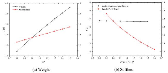
Fig.15 The effects of principal parameters on the natural heaving period. |
3.2. Second-level precontrol based on the green water height model
TLP roll and heave motions impact the relative position of the deck and wave surface. Therefore, short-period motion affects green water. Constraining green water involves two important steps: the development of a numerical model for green water height and the analysis of the influence laws of TLP parameters on green water height.
3.2.1. Mathematical model of TLP's green water height
The green water height can be represented by the opposite of the air gap δ( t) if it is less than the freeboard. The air gap δ( t) is defined as:
where δ0 is the initial static air gap and is the vertical distance between the bottom of the TLP's lower deck and wave surface at zero tide level, m; Ti is the maximum tide level, m; ξ7 is the maximum vertical drop of the deck and represents the vertical displacement of a position in the deck away from the centre of movement, m; ξ3( t) is the heave motion and represents the projection of the displacement of the TLP's movement centre in the vertical direction, m; and ξ0( t) is the wave surface, m (Fig. 16).

Fig.16 Definition of the air gap and a demonstration of waves slamming the lower deck of the TLP. |
The air gap is related to roll (impacting ξ7) and heave. The requirements for the TLP air gap are as follows: the minimum air gap should be greater than 1.5 m under sea conditions occurring once in a hundred years, and the minimum air gap should be greater than 0 m under sea conditions occurring once in a thousand years [12].
Waves slamming the TLP deck form green water. The random nature of waves makes it difficult to accurately predict green water. Wave height is determined by a stochastic process whose uncertainty hinders mathematical modelling of waves. The statistical approach addresses stochastic processes very well. It is assumed that waves are stationary and ergodic stochastic processes in time histories. Stochastic wave elevation is accumulated by infinite sine waves of random amplitude, period and initial phase, as shown in Fig. 17.
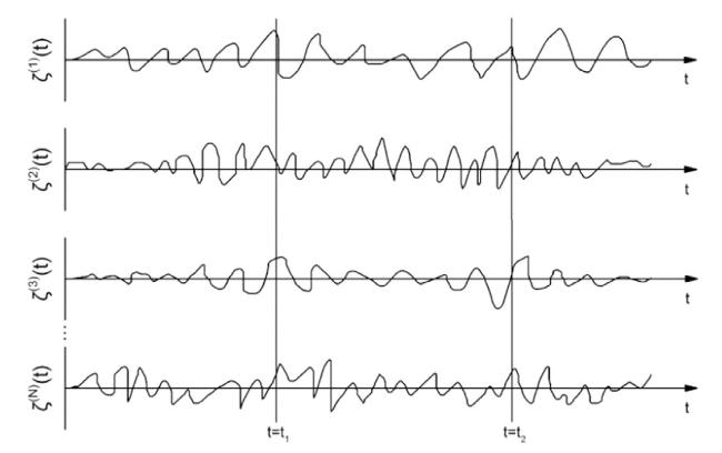
Fig.17 Random wave high superposition. |
Most wave energy is concentrated around a certain frequency. The wave spectral density function corresponds to a narrow band process. The wave spectrum is a stationary and ergodic process and follows a Rayleigh distribution.
The mean envelope curve amplitude is given by
The mean square envelope curve amplitude is given by
The variance of the wave spectrum with relative motion is given by
Waves are functions of time and space ξ0( x, t). The relative motion between the centre position of the TLP deck and the wave is described by
ξ3( t) and ξ0( x, t) are assumed to be harmonic functions of time and space. TLP's motion is described by
where is a complex number including amplitude and phase.
is the external wave excitation amplitude.
The relative motion between TLP and external wave excitation is described by
The response spectrum of the relative motion between the TLP and the wave is given by
Relative motion response amplitude operator | RAO( ω)| R represents TLP's motion in the Wave Lagrangian coordinate system, and it is the most important parameter for deriving the response spectrum of the relative motion between TLP and wave SR+( ω). | RAO( ω)|2 R is obtained by heave RAO and phase, which is calculated by hydrodynamic code (Fig. 18). Then, SR+( ω) is obtained using | RAO( ω)|2 R and Sω( m)++( ω0). Parameters, such as SR+( ω) standard variance σR, can be calculated afterwards. The green water height of the TLP deck centre position relative to the wave elevation is given by
where is the probability of a certain value being exceeded.
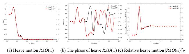
Fig.18 TLP heave motion RAO information. |
is the standard variance of the response spectrum of relative motion SR+( ω).
Green water height H is a function distributed in the frequency domain with exceeding probability as a parameter. This study calculates the mean height, upper control limit (UCL) height, and lower control limit (LCL) height of green water in the whole frequency domain by applying the mean area method. The mean area method transforms any distribution area into a rectangle of equal length and takes the rectangle's width as the mean height of green water (example shown in Fig. 19). Based on the variances calculated by the mean height of green water, the upper control limit height and lower control limit height of green water can be obtained with the PauTa Criterion (3σ Criterion). The interval between the upper control limit height and lower control limit height represents the possible maximum height range of green water. In summary, the three parameters - mean height, upper control limit height, and lower control limit height - represent the distribution characteristics of green water height.
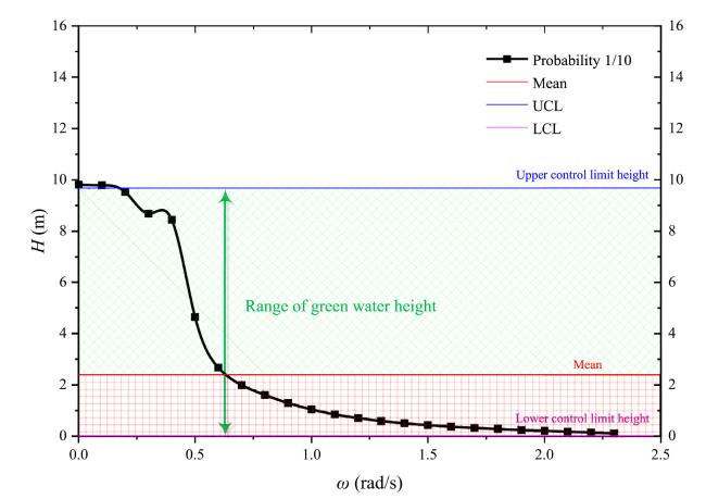
Fig.19 Green water height function distributed in the frequency domain with a probability of 1/10. |
3.2.2. Numerical implementation of green water height
To numerically implement the TLP's green water height, the mathematical model of the TLP's green water height requires the wave spectrum as input. In this study, the green water height is calculated using the JONSWAP spectrum (with γ=3.3) and the Pierson-Moskowitz spectrum as input. The JONSWAP spectrum is a growing spectrum and describes a growing wave height condition. The Pierson-Moskowitz spectrum is a fully developed spectrum and describes a stable wave height condition. For the same peak frequency, the average wave height calculated by the JONSWAP spectrum is approximately 23% higher than that calculated by the Pierson-Moskowitz spectrum [41]. The growing wave spectrum and developed wave spectrum can cover most wave conditions of green water. Parameters such as exceeding probability and wave incident angle are important representations of wave characteristics. The green water height is calculated by exceeding the 1/1000, 1/100, 1/10, and 1/3 probabilities, and the 0°, 45°, and 90° wave incident angles follow the JONSWAP spectrum and the Pierson-Moskowitz spectrum according to Eq. (19). The results are shown in Table 3. More details can be found in Wu's work [37].
Table 3 Information regarding green water obtained with the JONSWAP spectrum and the Pierson-Moskowitz spectrum. |
| Angle/° | Probability | JONSWAP spectrum | Pierson-Moskowitz spectrum | |||
|---|---|---|---|---|---|---|
| Mean/m | σ | Frequency/rad/s | Mean/m | Wind speed/m/s | ||
| 0 | 1/1000 | 4.15 | 3.193 | 0.635 | 4.15 | 14.35 |
| 1/100 | 3.39 | 2.885 | 0.635 | 3.39 | 14.35 | |
| 1/10 | 2.39 | 2.426 | 0.635 | 2.39 | 14.34 | |
| 1/3 | 1.65 | 2.016 | 0.635 | 1.65 | 14.34 | |
| 45 | 1/1000 | 4.21 | 3.209 | 0.635 | 4.21 | 14.35 |
| 1/100 | 3.44 | 2.900 | 0.635 | 3.44 | 14.35 | |
| 1/10 | 2.43 | 2.438 | 0.635 | 2.43 | 14.35 | |
| 1/3 | 1.68 | 2.026 | 0.635 | 1.68 | 14.35 | |
| 90 | 1/1000 | 4.15 | 3.193 | 0.635 | 4.15 | 14.35 |
| 1/100 | 3.39 | 2.885 | 0.635 | 3.39 | 14.35 | |
| 1/10 | 2.40 | 2.426 | 0.635 | 2.40 | 14.35 | |
| 1/3 | 1.65 | 2.016 | 0.635 | 1.65 | 14.35 | |
3.2.3. Green water height calculation
The mean heights of green water calculated by the JONSWAP spectrum and the Pierson-Moskowitz spectrum are approximately equal. This indicates that the distribution of wave energy is uniform in the time, space and frequency dimensions.
The drawing curves shown in Fig. 20 analyse the effects of exceeding probability and wave incident angle on the mean height and standard variance of green water. There is little effect of the wave incident angle on the mean height of green water. Because the TLP is symmetrical, the mean height of green water is the same as that of the four orthogonal symmetric direction waves. Conversely, exceeding probability has a considerable effect on the mean height of green water. As the exceeding probability increases, the mean height of green water decreases, and the slope decreases as well. Exceeding probability also has a strong effect on the standard variance of green water height. As the exceeding probability increases, the standard variance decreases. The wave incident angle has almost no influence on the standard variance of the green water height.
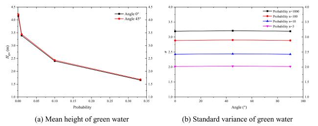
Fig.20 Influence of the wave incident angle and exceeding probability on the mean height and standard variance of green water. |
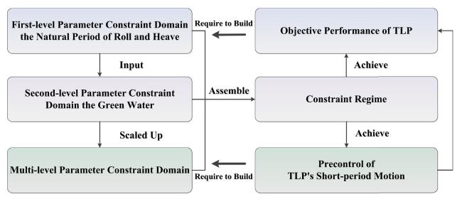
Fig.21 Constraint regime of the TLP's short-period motion. |
After numerical implementation, the mean height of green water was 2.34 m, and the corresponding exceeding probability was 1/8.5. To increase the green water height in the control, the upper control limit was set as the maximum σ, σ=3.209. The range of the green water height is 0∼11.967 m, and the corresponding probability is 99.73%, which means that the green water height is under control. The lower control limit is 0 m, the upper control limit is 11.967 m, and the corresponding probability is 99.73%. Thus, the actual probability of exceeding the upper control limit is 1/8.5 × (1-99.73%)=0.03%. This indicates that there is a very high probability that the green water height is in the range of 0∼11.967 m.
For this LH16-2 TLP project, the range of green water height is 0∼11.967 m. The maximum tide in the working sea area is 3.000 m. The TLP's freeboard is 19.850 m. The air gap without the tide effect is 7.883 m; the air gap modified by the tide is 4.883 m. Wang et al. carried out experimental research on the TLP's air gap [35]. Their experiment shows that the air gap without the tide effect is 4.540 m. TLP's air gap by the green water height numerical model is 7.883 m, the dimensionless moulded depth is 0.171, and their deviation is 42% (Table 4). Therefore, the numerical model of the green water height of the TLP is verified by the experiment to be accurate to the same order of magnitude.
Table 4 Experimental verification of the numerical model of the green water height of the TLP. |
| Items | Numerical Model/Dimensionless Moulded Depth | Experiment/Dimensionless Moulded Depth | Deviation |
|---|---|---|---|
| Air gap δ( t) (without tide effect) | 7.883 m/0.171 | 4.540 m/0.098 | 42% |
| Air gap δ( t) (with tide amendment) | 4.883 m/0.106 | 2.680 m/0.058 | 45% |
4. Discussion of the precontrol and constraint regime of TLP's short-period motion
TLP's short-period motion includes roll and heave motion that involve many sensitive motion modes, such as resonance and green water. The roll motion and the heave motion are related to dynamic stability, and green water relates to dynamic safety. In the previous section, the precontrol of short-period motion was decomposed into two-level constraints: roll and heave motion and green water. In this section, the multilevel parameter constraint domains (first-level parameter constraint domain natural period of roll and heave motion and second-level parameter constraint domain green water) are assembled into an entire constraint regime. The first-level parameter constraint domain is the input of the second-level parameter constraint domain; the second-level parameter constraint domain is the input of the third-level parameter constraint domain if more constraint levels are present. The parameter constraint domains are scaled up step by step as a constraint regime until all levels of precontrol objectives are covered. This constraint regime is used to achieve the precontrol objective (as shown in Fig. 21). If TLP's parameters are beyond the multilevel control range and within the feasible range, the performance of precontrol objectives can be achieved. This allows intervention before sensitive motion occurs to completely avoid the consequence of sensitive motion. Precontrol is a preventive control methodology that eliminates sensitive motion before it evolves into danger. Each level of the parameter constraint domain is stable. After all levels of parameter constraint domains, the range of parameters is further reduced. The input of the small range parameters of a stable system is convergent. Therefore, precontrol is a convergent methodology.
5. Conclusion
In this paper, a precontrol methodology is developed to constrain TLP's short-period motion prior to the occurrence of sensitive short-period motion. TLP's short-period motion includes roll and heave motions, and TLP faces the threat of resonance because the period of short-period motion is within the wave energy concentration region.
This study develops parameter-performance numerical models for short-period motion, such as the natural period of roll and heave model and green water height model, followed by experiments that validate the model fidelity. Based on these simple and high-fidelity numerical models, this study then investigated the influences of TLP parameters on the natural period and green water. The influence laws show that weight and stiffness significantly affect the natural period of the roll and the heave motion, and the wave's exceeding probability and initial static air gap significantly affect green water. Based on the influence laws and the range of sensitive short-period motion, a parameter constraint domain was generated that was divided into two parts: feasible range and control range. Two-level parameter constraint domains, namely, the first-level parameter constraint domain natural period of the roll and the heave motion and the second-level parameter constraint domain green water, were assembled into a constraint regime. In TLP design, the TLP's parameters are determined within a feasible range by bypassing the control range so that the TLP naturally exhibits motion performance that meets the requirements of short-period motion in advance, implementing the precontrol methodology.
Declaration of Competing Interest
The authors declare that they have no known competing financial interests or personal relationships that could have appeared to influence the work reported in this paper.
Acknowledgments
This study is supported by Kuaisu-Fuchi Project (Grant No. 80912020201) and Qingnian Yingcai Qihang Program.
