Research article

A novel approach to study generalized coupled cubic Schrödinger-Korteweg-de Vries equations

  • Lanre Akinyemi , a, * ,
  • P. Veeresha , b ,
  • M.T. Darvishi , c ,
  • Hadi Rezazadeh , d ,
  • Mehmet Şenol , e ,
  • Udoh Akpan , f
Expand
  • a Department of Mathematics, Lafayette College, Easton, PA, USA
  • b Department of Mathematics, Christ Deemed to be University, Bengaluru 560029, India
  • c Department of Mathematics, Razi University, Kermanshah 67149, Iran
  • d Faculty of Engineering Technology, Amol University of Special Modern Technologies, Amol, Iran
  • e Department of Mathematics, NevÅŸehir Hacı BektaÅŸ Veli University, NevÅŸehir, Turkey
  • f Drexel University, Department of Mathematics, Philadelphia, PA, USA
* E-mail addresses: (L. Akinyemi), (P. Veeresha), (M.T. Darvishi), (H. Rezazadeh), (M. Şenol), (U. Akpan).

Received date: 2022-05-05

  Revised date: 2022-05-29

  Accepted date: 2022-06-01

  Online published: 2024-11-13

Abstract

The Kortewegde Vries (KdV) equation represents the propagation of long waves in dispersive media, whereas the cubic nonlinear Schrödinger (CNLS) equation depicts the dynamics of narrow-bandwidth wave packets consisting of short dispersive waves. A model that couples these two equations seems intriguing for simulating the interaction of long and short waves, which is important in many domains of applied sciences and engineering, and such a system has been investigated in recent decades. This work uses a modified Sardar sub-equation procedure to secure the soliton-type solutions of the generalized cubic nonlinear Schrödinger-Korteweg-de Vries system of equations. For various selections of arbitrary parameters in these solutions, the dynamic properties of some acquired solutions are represented graphically and analyzed. In particular, the dynamics of the bright solitons, dark solitons, mixed bright-dark solitons, W-shaped solitons, M-shaped solitons, periodic waves, and other soliton-type solutions. Our results demonstrated that the proposed technique is highly efficient and effective for the aforementioned problems, as well as other nonlinear problems that may arise in the fields of mathematical physics and engineering.

Cite this article

Lanre Akinyemi , P. Veeresha , M.T. Darvishi , Hadi Rezazadeh , Mehmet Şenol , Udoh Akpan . A novel approach to study generalized coupled cubic Schrödinger-Korteweg-de Vries equations[J]. Journal of Ocean Engineering and Science, 2024 , 9(1) : 13 -24 . DOI: 10.1016/j.joes.2022.06.004

1. Introduction

Many topics in nonlinear science relating with ocean, aeronautical, mechanical, and many more may be characterized as solving nonlinear partial differential equations (NPDEs) that result from important models with mathematical and physical relevance. Solitons are one of the most frequently in the context of solutions for NPDEs, and they play a critical role in nonlinear physical phenomena exploration [1], [2], [3], [4], [5], [6], [7], [8], [9], [10], [11], [12], [13]. In disciplines including quantum electronics, plasma physics, nonlinear optics, fluid dynamics, and many more, solitons are used to better understand the nature of nonlinear media. In addition, soliton propagation has been used to explain several important oceanic phenomena that correlate to nonlinear shallow or deep-water wave propagation [14], [15], [16], [17]. In recent years, the search for accurate soliton solutions to NPDEs has become a fascinating study topic in the field of applied sciences and engineering. To examine such NPDEs, numerous well-established techniques have been offered such as the ansatz method [18], reduction of order method [19], tanh method [20], sine-Gordon method [21], extended auxiliary function method [22], Jacobi elliptic function method [23], F-expansion method [24], new extended direct algebraic method [25], ( G / G )-expansion method [26], homogeneous balance method [27], Lie symmetry method [28], sub-equation method [29], new Kudryashov’s method [30], simple equation method [31], Hirota bilinear method [32], and more.
One of the most general models for describing various physical nonlinear systems is the cubic nonlinear Schrödinger (CNLS) equation. This model has been used to better explain processes such as atomic physics and nonlinear optics, as well as deep sea waves, plasmas, rogue waves, and other phenomena. On the other hand, the KdV equation is one of the most prominent NPDEs. Examples include hydrodynamics, quantum field theory, plasma physics, water waves, and many more disciplines of applied sciences and engineering. It’s also utilized to explain the unidirectional propagation of long waves in nonlinear dispersive phenomena. In applied science and engineering, many types of coupled nonlinear systems have evolved as models for capturing interacting wave phenomena. Consequently, the coupled CNLS-KdV equations have been used to characterize a variety of wave phenomena in the aforementioned fields, including Langmuir waves, dust-acoustic waves, and electromagnetic waves in plasma physics, among others. They also appear in fluid mechanics phenomena such as the interactions of capillary gravity water waves, which involve short and long dispersive waves [33], [34], [35], [36], [37], [38].
In this work, the following generalized coupled CNLS-KdV equations are considered as:
i u t + α 1 u x x + α 2 | u | 2 u + α 3 u v = 0 , v t + γ 1 v v x + γ 2 v x x x + γ 3 ( | u | 2 ) x = 0 ,
where u = u ( x , t ) represents a complex function, and v = v ( x , t ) represents a real-valued function. The variables α j and γ j , j = 1 , 2 , 3 are all real constants. In addition, u denotes the short wave, and v represents the long wave. In [39], [40], the existence of solutions for the Eq. (1) was highlighted. The applications of Kudryashov and sub-equation methods to the proposed system have been published in Akinyemi et al. [41]. The numerical soutions with the help of q-homotopy analysis transform method was reported in Akinyemi et al. [42]. However, our aim is to further complement our previous study on Eq. (1) by proposing a modified Sardar sub-equation (MSSE) procedure to study this coupled system. The proposed method is an innovative technique for obtaining exact solutions to differential equations. It provides a straightforward approach for dealing with nonlinear evolution equation solutions. The SSE method has been used to obtain desirable findings and assistance in the investigation of solutions to numerous problems that have arisen in applied mathematics and physics [43], [44], [45]. Other advantage of this method is that it contain solutions reported in Akinyemi et al. [41], 42] and many other new soliton type solutions. These types of solutions are essential because they can aid in the understanding of several physical processes connected to wave propagation. It is important to highlight that the results acquired in this study are completely new and has never been published before. Kumar et al. [14] used the sine-Gordon equation approach to investigate the generalized Schrödinger–Boussinesq equations, which is another coupled model that describes the interaction between complex short and real long waves envelope.
The following is how the remainder of this paper is structured: Section 2 presents the description and application of recommended techniques. In Section 3, we will study several types of solitions type solutions of Eq. (1) with their valid constraint conditions, as well as discuss their dynamic characteristics using graphs, utilizing the MSSE method. Finally, in Section 5, the conclusion is provided.

2. The description of modified Sardar sub-equation method

This method is a powerful and robust approach that may be used to generate numerous types of soliton solutions, including dark, bright, W-shaped, mixed dark-bright, singular, mixed singular solitons, periodic, and other solutions, for both the classical and fractional order NPDEs as compared to other methods in the literature. The fact that this approach overcomes the complications of the solitary wave ansatz method [18], [46] is noteworthy. As a result, this section contains a full description of the MSSE approach. To use this approach, we assume the following general NPDE as:
G ( u , u t , u x , u x x , ) = 0 ,
where G denotes a function of u and its derivatives. The complex wave transformation [41] given as
u ( x , t ) = U ( ζ ) e i ( ω 2 x + η 2 t ) , ζ = ω 1 x + η 1 t ,
is proposed to reduce Eq. (2) into nonlinear ordinary differential equations (NODE):
N ( U , U , U , ) = 0 .
Here, U = U ( ζ ) denotes the amplitudes while ω j and η j , j = 1 , 2 are arbitrary constants. The solutions of Eq. (4) can be classify as:
ψ ( ζ ) = δ 0 + r = 1 M δ r Q r ( ζ ) , α M 0 ,
with the constants δ r , ( r = 0 , 1 , , M ) , ω j , and η j , ( j = 1 , 2 )are to be computed later. Balancing the highest-order derivative and the nonlinear terms of Eq. (4), determines the integer M . The function Q ( ζ ) in Eq. (5) satisfies
( Q ( ζ ) ) 2 = ϑ 2 Q 4 ( ζ ) + ϑ 1 Q 2 ( ζ ) + ϑ 0 ,
where ϑ 0 , ϑ 1 , and ϑ 2are constants. In addition, the family of solutions for Eq. (6) with constant ϱ are listed as below:
1. If ϑ 0 = 0 , ϑ 1 > 0 , and ϑ 2 0 , then
Q 1 ± ( ζ ) = ± ϑ 1 ϑ 2 sech ( ϑ 1 ( ζ + ϱ ) ) ,
Q 2 ± ( ζ ) = ± ϑ 1 ϑ 2 csch ( ϑ 1 ( ζ + ϱ ) ) .
2. For constants A 1 and A 2 . Let ϑ 2 = ± 4 A 1 A 2 , ϑ 1 > 0 , and ϑ 0 = 0 , we have
Q 3 ± ( ζ ) = ± 4 ϑ 1 A 1 ( 4 A 1 2 ϑ 2 ) cosh ( ϑ 1 ( ζ + ζ 0 ) ) ± ( 4 A 1 2 + ϑ 2 ) sinh ( ϑ 1 ( ζ + ζ 0 ) ) .
3. If ϑ 0 = ϑ 1 2 4 ϑ 2 , ϑ 1 < 0 , ϑ 2 > 0 , with constants B 1 , and B 2 , then
Q 3 ± ( ζ ) = ± ϑ 1 2 ϑ 2 tanh ( ϑ 1 2 ( ζ + ϱ ) ) ,
Q 4 ± ( ζ ) = ± ϑ 1 2 ϑ 2 coth ( ϑ 1 2 ( ζ + ϱ ) ) ,
Q 5 ± ( ζ ) = ± ϑ 1 2 ϑ 2 ( tanh ( 2 ϑ 1 ( ζ + ϱ ) ) ± i sech ( 2 ϑ 1 ( ζ + ϱ ) ) ) ,
Q 6 ( ζ ) = ± ϑ 1 8 ϑ 2 ( tanh ( ϑ 1 8 ( ζ + ϱ ) ) + coth ( ϑ 1 8 ( ζ + ϱ ) ) ) ,
Q 7 ± ( ζ ) = ± ϑ 1 2 ϑ 2 ( ± B 1 2 + B 2 2 B 1 cosh ( 2 ϑ 1 ( ζ + ϱ ) ) B 1 sinh ( 2 ϑ 1 ( ζ + ϱ ) ) + B 2 ) ,
Q 8 ± ( ζ ) = ± ϑ 1 2 ϑ 2 ( cosh ( 2 ϑ 1 ( ζ + ϱ ) ) sinh ( 2 ϑ 1 ( ζ + ϱ ) ) ± i ) .
4. If ϑ 0 = 0 , ϑ 1 < 0 , and ϑ 2 0 , then
Q 9 ± ( ζ ) = ± ϑ 1 ϑ 2 sec ( ϑ 1 ( ζ + ϱ ) ) ,
Q 10 ± ( ζ ) = ± ϑ 1 ϑ 2 csc ( ϑ 1 ( ζ + ϱ ) ) .
5. If ϑ 0 = ϑ 1 2 4 ϑ 2 , ϑ 1 > 0 , ϑ 2 > 0 , and B 1 2 B 2 2 > 0 , then
Q 11 ± ( ζ ) = ± ϑ 1 2 ϑ 2 tan ( ϑ 1 2 ( ζ + ϱ ) ) ,
Q 12 ± ( ζ ) = ± ϑ 1 2 ϑ 2 cot ( ϑ 1 2 ( ζ + ϱ ) ) ,
Q 13 ± ( ζ ) = ± ϑ 1 2 ϑ 2 ( tan ( 2 ϑ 1 ( ζ + ϱ ) ) ± sec ( 2 ϑ 1 ( ζ + ϱ ) ) ) ,
Q 14 ± ( ζ ) = ± ϑ 1 8 ϑ 2 ( tan ( ϑ 1 8 ( ζ + ϱ ) ) cot ( ϑ 1 8 ( ζ + ϱ ) ) ) ,
Q 15 ( ζ ) = ± ϑ 1 2 ϑ 2 ( ± B 1 2 B 2 2 B 1 cos ( 2 ϑ 1 ( ζ + ϱ ) ) B 1 sin ( 2 ϑ 1 ( ζ + ϱ ) ) + B 2 ) ,
Q 16 ( ζ ) = ± ϑ 1 2 ϑ 2 ( cos ( 2 ϑ 1 ( ζ + ϱ ) ) sin ( 2 ϑ 1 ( ζ + ϱ ) ) ± 1 ) .
6. If ϑ 0 = 0 and ϑ 1 > 0 , then
Q 17 ± ( ζ ) = 4 ϑ 1 e ± ϑ 1 ( ζ + ϱ ) e ± 2 ϑ 1 ( ζ + ϱ ) 4 ϑ 1 ϑ 2 ,
Q 18 ± ( ζ ) = ± 4 ϑ 1 e ± ϑ 1 ( ζ + ϱ ) 1 4 ϑ 1 ϑ 2 e ± 2 ϑ 1 ( ζ + ϱ ) .
7. If ϑ 0 = ϑ 1 = 0 and ϑ 2 > 0 , then
Q 19 ± ( ζ ) = ± 1 ϑ 2 ( ζ + ϱ ) .
8. If ϑ 0 = ϑ 1 = 0 and ϑ 2 < 0 , then
Q 20 ± ( ζ ) = ± i ϑ 2 ( ζ + ϱ ) .
Inserting Eqs. (5) and (6) into Eq. (4), then gathering and equating all the coefficients of Q r ( ζ ) to zero yields an algebraic system of equations in unknown variables δ r , ω j , and η j . After that, we solve the relevant set of equations, place the variables in Eq. (5), and use Eqs. (7)–(27) to obtain the precise solutions of Eq. (2).

3. The mathematical analysis and solutions

As presented in Eq. (1), the CNLS-KdV equations as a generalized coupled system:
i u t + α 1 u x x + α 2 | u | 2 u + α 3 u v = 0 , v t + γ 1 v v x + γ 2 v x x x + γ 3 ( | u | 2 ) x = 0 .
Because u is a complex function and v is a real-valued function, we suggest the transformation as follows:
u ( x , t ) = U ( ζ ) e i ( ω 2 x + η 2 t ) , v ( x , t ) = V ( ζ ) , ζ = ω 1 x + η 1 t ,
where ω j and η j , j = 1 , 2 are arbitrary constants. Using the transformation defined in Eq. (29), we obtain the real and imaginary parts of Eq. (28) as follows:
( η 2 + α 1 ω 2 2 ) U + α 1 ω 1 2 U + α 2 U 3 + α 3 U V = 0 ,
( η 1 + 2 α 1 ω 1 ω 2 ) U = 0 ,
and
η 1 V + γ 1 ω 1 V V + γ 2 ω 1 3 V ( 3 ) + 2 γ 3 ω 1 U U = 0 .
Solving Eq. (31) yields
η 1 = 2 α 1 ω 1 ω 2 .
Inserting Eq. (33) into Eq. (32), then integrating once while disregarding the integration constant results
2 α 1 ω 2 V + 1 2 γ 1 V 2 + γ 2 ω 1 2 V + γ 3 U 2 = 0 .
From Eq. (5), we can express the solutions of Eqs. (30) and (34) as:
U ( ζ ) = r = 0 M 1 f r Q r ( ζ ) , V ( ζ ) = r = 0 M 2 g r Q r ( ζ ) , g M 1 , g M 2 0 .
Here, f r and g r are constant to be evaluated later. Balancing U and U 3 in Eq. (30) results M 1 = 1 , while V and V 2 in Eq. (34) yields M 2 = 2 .
The solutions take the form
U ( ζ ) = f 0 + f 1 Q ( ζ ) , V ( ζ ) = g 0 + g 1 Q ( ζ ) + g 2 Q 2 ( ζ ) .
Putting Eqs. (6) and (36) into Eqs. (30) and (34), gathering all the coefficients of Q r ( ζ ) and setting them to zero, we get
Q 0 ( ζ ) : f 0 g 0 α 3 f 0 η 2 f 0 α 1 ω 2 2 + f 0 3 α 2 = 0 , : γ 3 f 0 2 + 2 γ 2 ϑ 0 g 2 ω 1 2 + 1 2 γ 1 g 0 2 2 g 0 α 1 ω 2 = 0 , Q 1 ( ζ ) : ϑ 1 f 1 α 1 ω 1 2 + f 0 g 1 α 3 + f 1 g 0 α 3 f 1 η 2 f 1 α 1 ω 2 2 + 3 f 1 f 0 2 α 2 = 0 , : 2 γ 3 f 0 f 1 + γ 2 ϑ 1 g 1 ω 1 2 + γ 1 g 0 g 1 2 g 1 α 1 ω 2 = 0 , Q 2 ( ζ ) : f 1 g 1 α 3 + f 0 g 2 α 3 + 3 f 0 f 1 2 α 2 = 0 , : γ 3 f 1 2 + 4 γ 2 ϑ 1 g 2 ω 1 2 + 1 2 γ 1 g 1 2 + γ 1 g 0 g 2 2 g 2 α 1 ω 2 = 0 , Q 3 ( ζ ) : 2 ϑ 2 f 1 α 1 ω 1 2 + f 1 g 2 α 3 + f 1 3 α 2 = 0 , : 2 γ 2 ϑ 2 g 1 ω 1 2 + γ 1 g 1 g 2 = 0 , Q 4 ( ζ ) : 6 γ 2 ϑ 2 g 2 ω 1 2 + 1 2 γ 1 g 2 2 = 0 .
The solutions to the aforementioned algebraic equations using Mathematica, along with Eq. (33) yield the following results:
Case 1.
η 1 = 2 α 1 ω 1 ω 2 , η 2 = ϑ 1 α 1 ω 1 2 + 12 γ 2 2 ϑ 0 ϑ 2 ω 1 4 α 1 4 γ 2 ϑ 1 α 3 ω 1 2 γ 1 ( 24 γ 2 2 ϑ 1 α 2 ω 1 2 + γ 3 ( γ 1 α 1 6 γ 2 α 3 ) ) 2 144 γ 2 2 α 1 α 2 2 + γ 3 α 3 2 γ 1 α 2 γ 3 α 1 α 3 6 γ 2 α 2 α 3 γ 1 2 ( 576 γ 2 4 ( ϑ 1 2 3 ϑ 0 ϑ 2 ) α 2 2 ω 1 4 + 48 γ 2 2 γ 3 ϑ 1 α 2 ω 1 2 ( γ 1 α 1 6 γ 2 α 3 ) + γ 3 2 ( γ 1 α 1 6 γ 2 α 3 ) 2 ) 6 γ 1 2 γ 2 α 2 , g 0 = 1 6 γ 1 2 γ 2 α 2 ( 24 γ 2 2 γ 1 ϑ 1 α 2 ω 1 2 + 6 γ 2 γ 3 γ 1 α 3 γ 1 2 γ 3 α 1 ( 24 γ 2 2 γ 1 ϑ 1 α 2 ω 1 2 + γ 3 γ 1 2 α 1 6 γ 2 γ 3 γ 1 α 3 ) 2 1728 γ 1 2 γ 2 4 ϑ 0 ϑ 2 α 2 2 ω 1 4 ) , g 1 = 0 , g 2 = 12 γ 2 ϑ 2 ω 1 2 γ 1 , f 0 = 0 , f 1 = i ω 1 2 ϑ 2 ( γ 1 α 1 6 γ 2 α 3 ) γ 1 α 2 , ω 2 = ( 24 γ 2 2 γ 1 ϑ 1 α 2 ω 1 2 + γ 3 γ 1 2 α 1 6 γ 2 γ 3 γ 1 α 3 ) 2 1728 γ 1 2 γ 2 4 ϑ 0 ϑ 2 α 2 2 ω 1 4 12 γ 1 γ 2 α 1 α 2 .
Case 2.
η 1 = 2 α 1 ω 1 ω 2 , η 2 = ϑ 1 α 1 ω 1 2 + 12 γ 2 2 ϑ 0 ϑ 2 ω 1 4 α 1 4 γ 2 ϑ 1 α 3 ω 1 2 γ 1 ( 24 γ 2 2 ϑ 1 α 2 ω 1 2 + γ 3 ( γ 1 α 1 6 γ 2 α 3 ) ) 2 144 γ 2 2 α 1 α 2 2 + γ 3 α 3 2 γ 1 α 2 γ 3 α 1 α 3 6 γ 2 α 2 + α 3 γ 1 2 ( 576 γ 2 4 ( ϑ 1 2 3 ϑ 0 ϑ 2 ) α 2 2 ω 1 4 + 48 γ 2 2 γ 3 ϑ 1 α 2 ω 1 2 ( γ 1 α 1 6 γ 2 α 3 ) + γ 3 2 ( γ 1 α 1 6 γ 2 α 3 ) 2 ) 6 γ 1 2 γ 2 α 2 , g 0 = 1 6 γ 1 2 γ 2 α 2 ( 24 γ 2 2 γ 1 ϑ 1 α 2 ω 1 2 + 6 γ 2 γ 3 γ 1 α 3 γ 1 2 γ 3 α 1 + ( 24 γ 2 2 γ 1 ϑ 1 α 2 ω 1 2 + γ 3 γ 1 2 α 1 6 γ 2 γ 3 γ 1 α 3 ) 2 1728 γ 1 2 γ 2 4 ϑ 0 ϑ 2 α 2 2 ω 1 4 ) , g 1 = 0 , g 2 = 12 γ 2 ϑ 2 ω 1 2 γ 1 , f 0 = 0 , f 1 = i ω 1 2 ϑ 2 ( γ 1 α 1 6 γ 2 α 3 ) γ 1 α 2 , ω 2 = ( 24 γ 2 2 γ 1 ϑ 1 α 2 ω 1 2 + γ 3 γ 1 2 α 1 6 γ 2 γ 3 γ 1 α 3 ) 2 1728 γ 1 2 γ 2 4 ϑ 0 ϑ 2 α 2 2 ω 1 4 12 γ 1 γ 2 α 1 α 2 .
By incorporating the parameters in Case 1 into Eq. (36), in addition to Eqs. (7)–(27), we have the following solutions:
The bright and singular solitons can be consider as:
u 1 ( x , t ) = ω 1 2 ϑ 1 ( γ 1 α 1 6 γ 2 α 3 ) γ 1 α 2 sech ( ϑ 1 ( ζ + ϱ ) ) e i ( ω 2 x + η 2 t ) , v 1 ( x , t ) = g 0 + 12 γ 2 ϑ 1 ω 1 2 γ 1 sech 2 ( ϑ 1 ( ζ + ϱ ) ) ,
u 2 ( x , t ) = i ω 1 2 ϑ 1 ( γ 1 α 1 6 γ 2 α 3 ) γ 1 α 2 csch ( ϑ 1 ( ζ + ϱ ) ) e i ( ω 2 x + η 2 t ) , v 2 ( x , t ) = g 0 12 γ 2 ϑ 1 ω 1 2 γ 1 csch 2 ( ϑ 1 ( ζ + ϱ ) ) ,
where ζ = ω 1 x + η 1 t , ϑ 0 = 0 , ϑ 1 > 0 , and ϑ 2 0 .
The dark and singular solitons can be consider as:
u 3 ( x , t ) = i ω 1 ϑ 1 ( γ 1 α 1 6 γ 2 α 3 ) γ 1 α 2 tanh ( ϑ 1 2 ( ζ + ϱ ) ) e i ( ω 2 x + η 2 t ) , v 3 ( x , t ) = H 1 + 6 γ 2 ϑ 1 ω 1 2 γ 1 tanh 2 ( ϑ 1 2 ( ζ + ϱ ) ) ,
u 4 ( x , t ) = i ω 1 ϑ 1 ( γ 1 α 1 6 γ 2 α 3 ) γ 1 α 2 coth ( ϑ 1 2 ( ζ + ϱ ) ) e i ( ω 2 x + η 2 t ) , v 4 ( x , t ) = H 1 + 6 γ 2 ϑ 1 ω 1 2 γ 1 coth 2 ( ϑ 1 2 ( ζ + ϱ ) ) ,
where ϑ 0 = ϑ 1 2 4 ϑ 2 , ϑ 1 < 0 , ϑ 2 > 0 , and H 1 = 6 γ 2 γ 1 ( 4 γ 2 ϑ 1 α 2 ω 1 2 γ 3 α 3 ) + γ 1 2 ( ( 24 γ 2 2 ϑ 1 α 2 ω 1 2 + γ 3 ( γ 1 α 1 6 γ 2 α 3 ) ) 2 432 γ 2 4 ϑ 1 2 α 2 2 ω 1 4 ) + γ 3 γ 1 2 α 1 6 γ 1 2 γ 2 α 2 .
The combo bright-singular solitons are expressed as:
u 5 ( x , t ) = 4 i ω 1 A 1 2 ϑ 1 ϑ 2 ( γ 1 α 1 6 γ 2 α 3 ) e i ( ω 2 x + η 2 t ) γ 1 α 2 ( ( 4 A 1 2 + ϑ 2 ) sinh ( ϑ 1 ( ζ + ϱ ) ) ± ( 4 A 1 2 ϑ 2 ) cosh ( ϑ 1 ( ζ + ϱ ) ) ) , v 5 ( x , t ) = H 2 192 γ 2 ϑ 1 ϑ 2 ω 1 2 A 1 2 γ 1 ( ( 4 A 1 2 + ϑ 2 ) sinh ( ϑ 1 ( ζ + ϱ ) ) ± ( 4 A 1 2 ϑ 2 ) cosh ( ϑ 1 ( ζ + ϱ ) ) ) 2 ,
where ϑ 0 = 0 , ϑ 1 > 0 , ϑ 2 = ± 4 A 1 A 2 , and H 2 = 6 γ 2 γ 1 ( 4 γ 2 ϑ 1 α 2 ω 1 2 γ 3 α 3 ) + γ 1 2 ( 24 γ 2 2 ϑ 1 α 2 ω 1 2 + γ 3 ( γ 1 α 1 6 γ 2 α 3 ) ) 2 + γ 3 γ 1 2 α 1 6 γ 1 2 γ 2 α 2 .
The combo solitons are as follows:
u 6 ( x , t ) = i ω 1 ϑ 1 ( γ 1 α 1 6 γ 2 α 3 ) γ 1 α 2 ( tanh ( 2 ϑ 1 ( ζ + ϱ ) ) ± i sech ( 2 ϑ 1 ( ζ + ϱ ) ) ) e i ( ω 2 x + η 2 t ) , v 6 ( x , t ) = H 1 + 6 γ 2 ϑ 1 ω 1 2 γ 1 ( tanh ( 2 ϑ 1 ( ζ + ϱ ) ) ± i sech ( 2 ϑ 1 ( ζ + ϱ ) ) ) 2 ,
u 7 ( x , t ) = i ω 1 2 ϑ 1 ( γ 1 α 1 6 γ 2 α 3 ) γ 1 α 2 ( tanh ( ϑ 1 8 ( ζ + ϱ ) ) + coth ( ϑ 1 8 ( ζ + ϱ ) ) ) e i ( ω 2 x + η 2 t ) , v 7 ( x , t ) = H 1 + 3 γ 2 ϑ 1 ω 1 2 2 γ 1 ( tanh ( ϑ 1 8 ( ζ + ϱ ) ) + coth ( ϑ 1 8 ( ζ + ϱ ) ) ) 2 ,
u 8 ( x , t ) = i ω 1 ϑ 1 ( γ 1 α 1 6 γ 2 α 3 ) γ 1 α 2 ( ± B 1 2 + B 2 2 B 1 cosh ( 2 ϑ 1 ( ζ + ϱ ) ) B 1 sinh ( 2 ϑ 1 ( ζ + ϱ ) ) + B 2 ) e i ( ω 2 x + η 2 t ) , v 8 ( x , t ) = H 1 + 6 γ 2 ϑ 1 ω 1 2 γ 1 ( ± B 1 2 + B 2 2 B 1 cosh ( 2 ϑ 1 ( ζ + ϱ ) ) B 1 sinh ( 2 ϑ 1 ( ζ + ϱ ) ) + B 2 ) 2 ,
u 9 ( x , t ) = i ω 1 ϑ 1 ( γ 1 α 1 6 γ 2 α 3 ) γ 1 α 2 ( cosh ( 2 ϑ 1 ( ζ + ϱ ) ) sinh ( 2 ϑ 1 ( ζ + ϱ ) ) ± i ) e i ( ω 2 x + η 2 t ) , v 9 ( x , t ) = H 1 + 6 γ 2 ϑ 1 ω 1 2 γ 1 ( cosh ( 2 ϑ 1 ( ζ + ϱ ) ) sinh ( 2 ϑ 1 ( ζ + ϱ ) ) ± i ) 2 ,
where ϑ 0 = ϑ 1 2 4 ϑ 2 , ϑ 1 < 0 , ϑ 2 > 0 , and H 1 = 6 γ 2 γ 1 ( 4 γ 2 ϑ 1 α 2 ω 1 2 γ 3 α 3 ) + γ 1 2 ( ( 24 γ 2 2 ϑ 1 α 2 ω 1 2 + γ 3 ( γ 1 α 1 6 γ 2 α 3 ) ) 2 432 γ 2 4 ϑ 1 2 α 2 2 ω 1 4 ) + γ 3 γ 1 2 α 1 6 γ 1 2 γ 2 α 2 .
The trigonometric function solutions are acquired as follows:
u 10 ( x , t ) = i ω 1 2 ϑ 1 ( γ 1 α 1 6 γ 2 α 3 ) γ 1 α 2 sec ( ϑ 1 ( ζ + ϱ ) ) e i ( ω 2 x + η 2 t ) , v 10 ( x , t ) = H 2 + 12 γ 2 ϑ 1 ω 1 2 γ 1 sec 2 ( ϑ 1 ( ζ + ϱ ) ) ,
u 11 ( x , t ) = i ω 1 2 ϑ 1 ( γ 1 α 1 6 γ 2 α 3 ) γ 1 α 2 csc ( ϑ 1 ( ζ + ϱ ) ) e i ( ω 2 x + η 2 t ) , v 11 ( x , t ) = H 2 + 12 γ 2 ϑ 1 ω 1 2 γ 1 csc 2 ( ϑ 1 ( ζ + ϱ ) ) ,
for ϑ 0 = 0 , ϑ 1 < 0 , and ϑ 2 0 , and H 2 = 6 γ 2 γ 1 ( 4 γ 2 ϑ 1 α 2 ω 1 2 γ 3 α 3 ) + γ 1 2 ( 24 γ 2 2 ϑ 1 α 2 ω 1 2 + γ 3 ( γ 1 α 1 6 γ 2 α 3 ) ) 2 + γ 3 γ 1 2 α 1 6 γ 1 2 γ 2 α 2 .
u 12 ( x , t ) = i ω 1 ϑ 1 ( γ 1 α 1 6 γ 2 α 3 ) γ 1 α 2 tan ( ϑ 1 2 ( ζ + ϱ ) ) e i ( ω 2 x + η 2 t ) , v 12 ( x , t ) = H 1 12 γ 2 ϑ 1 ω 1 2 γ 1 tan 2 ( ϑ 1 2 ( ζ + ϱ ) ) ,
u 13 ( x , t ) = i ω 1 ϑ 1 ( γ 1 α 1 6 γ 2 α 3 ) γ 1 α 2 cot ( ϑ 1 2 ( ζ + ϱ ) ) e i ( ω 2 x + η 2 t ) , v 13 ( x , t ) = H 1 12 γ 2 ϑ 1 ω 1 2 γ 1 cot 2 ( ϑ 1 2 ( ζ + ϱ ) ) ,
for ϑ 0 = ϑ 1 2 4 ϑ 2 , ϑ 1 > 0 , ϑ 2 > 0 , and H 1 = 6 γ 2 γ 1 ( 4 γ 2 ϑ 1 α 2 ω 1 2 γ 3 α 3 ) + γ 1 2 ( ( 24 γ 2 2 ϑ 1 α 2 ω 1 2 + γ 3 ( γ 1 α 1 6 γ 2 α 3 ) ) 2 432 γ 2 4 ϑ 1 2 α 2 2 ω 1 4 ) + γ 3 γ 1 2 α 1 6 γ 1 2 γ 2 α 2 .
The mixed trigonometric function solutions are as follows:
u 14 ( x , t ) = i ω 1 ϑ 1 ( γ 1 α 1 6 γ 2 α 3 ) γ 1 α 2 ( tan ( 2 ϑ 1 ( ζ + ϱ ) ) ± sec ( 2 ϑ 1 ( ζ + ϱ ) ) ) e i ( ω 2 x + η 2 t ) , v 14 ( x , t ) = H 1 6 γ 2 ϑ 1 ω 1 2 γ 1 ( tan ( 2 ϑ 1 ( ζ + ϱ ) ) ± sec ( 2 ϑ 1 ( ζ + ϱ ) ) ) 2 ,
u 15 ( x , t ) = i ω 1 2 ϑ 1 ( γ 1 α 1 6 γ 2 α 3 ) γ 1 α 2 ( tan ( ϑ 1 8 ( ζ + ϱ ) ) cot ( ϑ 1 8 ( ζ + ϱ ) ) ) e i ( ω 2 x + η 2 t ) , v 15 ( x , t ) = H 1 3 γ 2 ϑ 1 ω 1 2 2 γ 1 ( tan ( ϑ 1 8 ( ζ + ϱ ) ) cot ( ϑ 1 8 ( ζ + ϱ ) ) ) 2 ,
u 16 ( x , t ) = i ω 1 ϑ 1 ( γ 1 α 1 6 γ 2 α 3 ) γ 1 α 2 ( ± B 1 2 B 2 2 B 1 cos ( 2 ϑ 1 ( ζ + ϱ ) ) B 1 sin ( 2 ϑ 1 ( ζ + ϱ ) ) + B 2 ) e i ( ω 2 x + η 2 t ) , v 16 ( x , t ) = H 1 6 γ 2 ϑ 1 ω 1 2 γ 1 ( ± B 1 2 B 2 2 B 1 cos ( 2 ϑ 1 ( ζ + ϱ ) ) B 1 sin ( 2 ϑ 1 ( ζ + ϱ ) ) + B 2 ) 2 ,
u 17 ( x , t ) = i ω 1 ϑ 1 ( γ 1 α 1 6 γ 2 α 3 ) γ 1 α 2 ( cos ( 2 ϑ 1 ( ζ + ϱ ) ) sin ( 2 ϑ 1 ( ζ + ϱ ) ) ± 1 ) e i ( ω 2 x + η 2 t ) , v 17 ( x , t ) = H 1 6 γ 2 ϑ 1 ω 1 2 γ 1 ( cos ( 2 ϑ 1 ( ζ + ϱ ) ) sin ( 2 ϑ 1 ( ζ + ϱ ) ) ± 1 ) 2 ,
where ϑ 0 = 0 , ϑ 1 < 0 , ϑ 2 0 , and H 1 = 6 γ 2 γ 1 ( 4 γ 2 ϑ 1 α 2 ω 1 2 γ 3 α 3 ) + γ 1 2 ( ( 24 γ 2 2 ϑ 1 α 2 ω 1 2 + γ 3 ( γ 1 α 1 6 γ 2 α 3 ) ) 2 432 γ 2 4 ϑ 1 2 α 2 2 ω 1 4 ) + γ 3 γ 1 2 α 1 6 γ 1 2 γ 2 α 2 .
The exponential solutions are:
u 18 ( x , t ) = 4 i ϑ 1 ω 1 2 ϑ 2 ( γ 1 α 1 6 γ 2 α 3 ) γ 1 α 2 e ϑ 1 ( ζ + ϱ ) e 2 ϑ 1 ( ζ + ϱ ) 4 ϑ 1 ϑ 2 e i ( ω 2 x + η 2 t ) , v 18 ( x , t ) = H 2 192 γ 2 ϑ 1 2 ϑ 2 ω 1 2 e 2 ϑ 1 ( ζ + ϱ ) γ 1 ( e 2 ϑ 1 ( ζ + ϱ ) 4 ϑ 1 ϑ 2 ) 2 ,
u 19 ( x , t ) = 4 i ϑ 1 ω 1 2 ϑ 2 ( γ 1 α 1 6 γ 2 α 3 ) γ 1 α 2 e ± ϑ 1 ( ζ + ϱ ) 1 4 ϑ 1 ϑ 2 e ± 2 ϑ 1 ( ζ + ϱ ) e i ( ω 2 x + η 2 t ) , v 19 ( x , t ) = H 2 192 γ 2 ϑ 1 2 ϑ 2 ω 1 2 e ± 2 ϑ 1 ( ζ + ϱ ) γ 1 ( 1 4 ϑ 1 ϑ 2 e ± 2 ϑ 1 ( ζ + ϱ ) ) 2 ,
where ϑ 0 = 0 , ϑ 1 > 0 , ϑ 2 0 , and H 2 = 6 γ 2 γ 1 ( 4 γ 2 ϑ 1 α 2 ω 1 2 γ 3 α 3 ) + γ 1 2 ( 24 γ 2 2 ϑ 1 α 2 ω 1 2 + γ 3 ( γ 1 α 1 6 γ 2 α 3 ) ) 2 + γ 3 γ 1 2 α 1 6 γ 1 2 γ 2 α 2 .
The rational solutions are:
u 20 ( x , t ) = i ω 1 2 ( γ 1 α 1 6 γ 2 α 3 ) γ 1 α 2 ζ + ϱ e i ( ω 2 x + η 2 t ) , v 20 ( x , t ) = H 3 12 γ 2 ω 1 2 γ 1 ( ζ + ϱ ) 2 ,
for ϑ 0 = ϑ 1 = 0 , ϑ 2 > 0 , and H 3 = γ 3 γ 1 2 α 1 6 γ 2 γ 3 γ 1 α 3 + γ 1 2 γ 3 2 ( γ 1 α 1 6 γ 2 α 3 ) 2 6 γ 1 2 γ 2 α 2 .

4. Result and discussion

In this work, several graphs are displayed using Mathematica to examine the behavior of the solitons and comprehend the physical meaning of the obtained solutions by selecting appropriate values for unknown parameters. The 3D and 2D plots for Eqs. (40), (42), (49), (40), and (51) are depicted through Fig. 1, Fig. 2, Fig. 3, Fig. 4, Fig. 5, Fig. 6, Fig. 7, Fig. 8, Fig. 9, Fig. 10 which reveal different wave structures that are of important in the field of applied sciences and engineering. These plots present various forms of solutions such as the bright soliton, dark soliton, W-shaped soliton, M-shaped soliton, mixed bright-dark soliton, singular soliton, periodic wave, and other soliton-type solutions. The suitable parameters used for these plots are as follows:
• Figs. 1 and 2 with ω 1 = 0.1 , α 1 = α 2 = 1 , α 3 = 1 , γ 1 = 1 , γ 2 = γ 3 = 1 , ϑ 1 = 0.5 , and ϱ = 0.01 .
Fig. 3, Fig. 4, Fig. 5, Fig. 6 with ω 1 = 0.1 , α 1 = α 2 = 1 , α 3 = 1 , γ 1 = 1 , γ 2 = γ 3 = 1 , ϑ 1 = 2 , and ϱ = 0.01 .
•Figs. 7 and 8 with ω 1 = 0.1 , α 1 = 1 , α 2 = 2 , α 3 = γ 1 = 1 , γ 2 = 1 , γ 3 = 1 , ϑ 1 = 5 , and ϱ = 0.01 .
•Figs. 9 and 10 with ω 1 = 0.1 , α 1 = 1 , α 2 = 2 , α 3 = γ 1 = γ 3 = 1 , γ 2 = 1 , ϑ 1 = 5 , and ϱ = 0.01 .
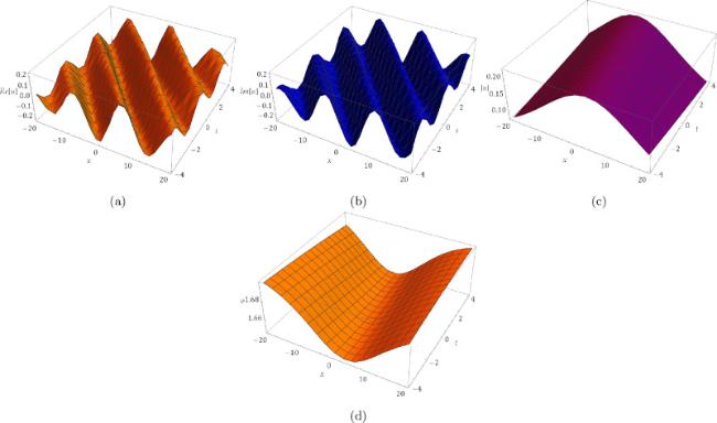
Fig.1 3D wave simulations of Eq. (40) solutions.
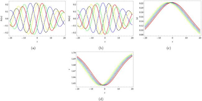
Fig. 2. 2D wave simulations of Eq. (40) solutions
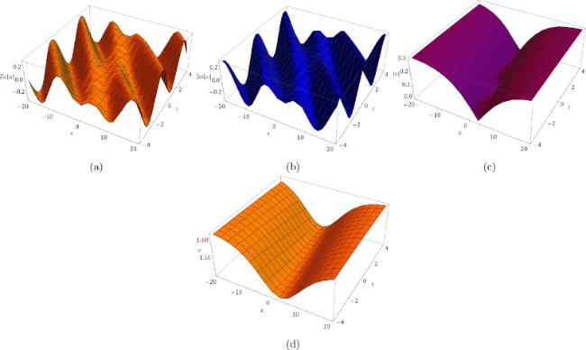
Fig. 3. 3D wave simulations of Eq. (42) solutions
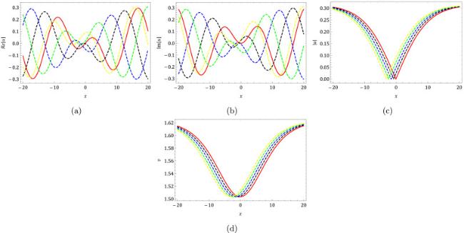
Fig. 4. 2D wave simulations of Eq. (42) solutions
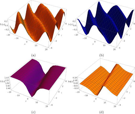
Fig. 5. 3D wave simulations of Eq. (45) solutions
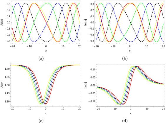
Fig. 6. 2D wave simulations of Eq. (45) solutions
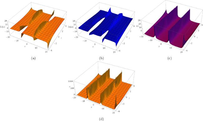
Fig. 7. 3D wave simulations of Eq. (49) solutions
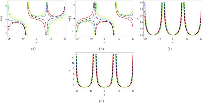
Fig. 8. 2D wave simulations of Eq. (49) solutions
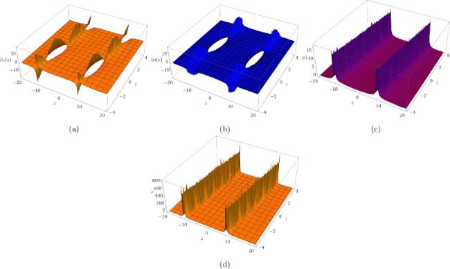
Fig. 9. 3D wave simulations of Eq. (51) solutions
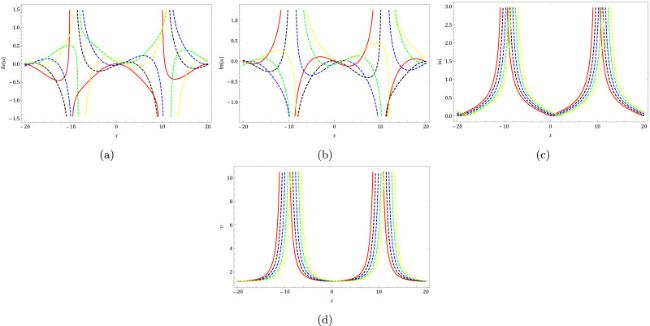
Fig. 10. 2D wave simulations of Eq. (51) solutions
Furthermore, all 2D graphs are shown with different t values which are t = 0 (solid red), t = 1 (dashed Black), t = 2 (dashed blue), t = 3 (dashed green), and t = 4 (dashed yellow) respectively. The graphical outputs show that the suggested method will contribute to other related strong nonlinear models in order to generate some new soliton solutions. As a consequence, it is abundantly obvious that the obtained results in this study provide new information to the current literature due to their relevance in the aforementioned disciplines.

5. Conclusion

The MSSE approach is used in this work to acquire novel and significant solutions to the generalized coupled CNLS-KdV equations. In particular, we obtain the bright soliton, dark solitons, W-shaped solitons, M-shaped solitons, mixed bright-dark solitons, singular solitons, periodic wave, and other soliton-type solutions. These solutions are provided for Case 1, and a similar approach may be used for Case 2, where several novel solitons and other solutions can be retrieve as well. The advantage of this method is that it contain the solutions reported in Akinyemi et al. [41] and also present new ones. Graphical representations in 2D and 3D plots as illustrated in Fig. 1, Fig. 2, Fig. 3, Fig. 4, Fig. 5, Fig. 6, Fig. 7, Fig. 8, Fig. 9, Fig. 10 are given to comprehend the appropriate relevance of the suggested method through some accomplished soliton solutions. These solutions will likely play an important role in understanding the dynamics of this coupled model and capturing some of its physical properties. The acquired results cab be beneficial for a deeper understanding of the interacting wave phenomenon in any variety of situations where the coupled model under consideration is relevant. It’s also worth noting that the recovered solution’s authenticity is verified by plugging the acquired exact solutions back into the original equation.

Declaration of Competing Interest

The authors declare that they have no known competing financial interests or personal relationships that could have appeared to influence the work reported in this paper.
[1]
M.J. Ablowitz, B. Prinari, A.D. Trubatch. Discrete and Continuous Nonlinear Schrödinger Systems. Cambridge University Press, Cambridge (2004)

[2]
M.J. Ablowitz. Nonlinear Dispersive Waves:Asymptotic Analysis and Solitons. Cambridge University Press, Cambridge (2011)

[3]
A. Biswas, D. Milovic. Commun. Nonlinear Sci. Numer. Simul., 15 (2010), pp. 1473-1484

[4]
A. Biswas. Optik, 176 (2019), pp. 198-201

[5]
H.H. Dai. Acta Mech., 127 (1998), pp. 193-207

[6]
W.P. Hong. Opt. Commun., 194 (2001), pp. 217-223

[7]
M. Inc, M.N. Khan, I. Ahmad, S.W. Yao, H. Ahmad, P. Thounthong. Res. Phys., 19 (2020) Article 103385

[8]
A.M. Wazwaz. Optik, 192 (2019), pp. 1-5

[9]
A.M. Wazwaz. Optik, 225 (2021), pp. 1-5 DOI: 10.1109/irec52758.2021.9624925

[10]
H. Rezazadeh, A. Korkmaz, A.E. Achab, W. Adel, A. Bekir. Appl. Math. Nonlinear Sci., 6 (1) (2021), pp. 447-458 DOI: 10.2478/amns.2020.2.00034

[11]
H.U. Rehman, M. Bibi, M.S. Saleem, H. Rezazadeh, W. Adel, Int. J. Mod. Phys. B, 35 (18) (2021) Article 2150184

[12]
K. Hosseini, M. Mirzazadeh, D. Baleanu, S. Salahshour, L. Akinyemi. Opt. Quant. Electron., 54 (3) (2022), pp. 1-12

[13]
S.W. Yao, L. Akinyemi, M. Mirzazadeh, M. Inc, K. Hosseini, M. Aenol. Res. Phys., 30 (2021) Article 104825

[14]
D. Kumar, K. Hosseini, M.K. Kaabar, M. Kaplan, S. Salahshour. J. Ocean Eng. Sci. (2021), DOI: 10.1016/j.joes.2021.09.008

[15]
A.M. Wazwaz. Ocean Eng., 53 (2012), pp. 1-5

[16]
S. Kumar, S. Rani. J. Ocean Eng. Sci. (2021), DOI: 10.1016/j.joes.2021.10.002.

[17]
L. Akinyemi, M. Ã…enol, U. Akpan, H. Rezazadeh. J. Ocean Eng. Sci. (2022), DOI: 10.1016/j.joes.2022.04.023.

[18]
A. Bekir,. A. Gner. Ocean Eng., 74 (2013), pp. 276-279

[19]
M. Inc, B. Kilic. Waves Random Complex Media, 27 (1) (2017), pp. 28-37 DOI: 10.1080/17455030.2016.1186855

[20]
A.M. Wazwaz. Appl. Math. Lett., 19 (2006), pp. 1162-1167

[21]
H. Rezazadeh, W. Adel, M. Eslami, K.U. Tariq, S.M. Mirhosseini-Alizamini, A. Bekir, Y.M. Chu. Open Phys., 19 (1) (2021), pp. 111-118 DOI: 10.1515/phys-2021-0013

[22]
X. Yang, C. Zhao, J. Cao. Appl. Math. Comput., 219 (16) (2013), pp. 8508-8524

[23]
E.A. Az-Zobi, W.A. AlZoubi, L. Akinyemi, et al.. Opt. Quant. Electron., 53 (132) (2021), pp. 1-16, DOI:

[24]
D. Lu, Z. Zhang. Int. J. Nonlinear Sci., 24 (2) (2017), pp. 96-103

[25]
H. Rezazadeh. Optik, 167 (2018), pp. 218-227

[26]
A. Bekir, O. Guner. Chin. Phys. B, 22 (11) (2013), pp. 1-6 DOI: 10.1155/2013/426462

[27]
H. Jafari, H. Tajadodi, D. Baleanu. J. Comput. Nonlinear Dyn., 9 (2) (2014), pp. 021019-21021

[28]
F. Tchier, A. Yusuf, A.I. Aliyu, M. Inc. Superlattices Microstruct., 107 (2017), pp. 320-336

[29]
E.M. Zayed, A.G. Al-Nowehy, R.M. Shohib. J. Ocean Eng. Sci., 4 (1) (2019), pp. 14-23

[30]
H. Rezazadeh, N. Ullah, L. Akinyemi, A. Shah, S.M. Mirhosseini-Alizamin, Y.M. Chu, H. Ahmad. Res. Phys., 24 (2021), Article 104179

[31]
L. Akinyemi, M. Mirzazadeh, K. Hosseini. Nonlinear Anal., 27 (2022), pp. 1-17 DOI: 10.15388/namc.2022.27.26374

[32]
H.F. Ismael, H. Bulut, M.S. Osman. Nonlinear Dyn., 107 (4) (2022), pp. 3791-3803 DOI: 10.1007/s11071-021-07154-z

[33]
N.V. Nguyen, C. Liu. Water Waves, 2 (2020), pp. 327-359 DOI: 10.1007/s42286-020-00038-6

[34]
J. Albert, J.A. Pava. Proc. R. Soc. Edinburgh Sect. A, 133 (5) (2003), pp. 987-1029

[35]
A.J. Corcho, F. Linares. Trans. Am. Math. Soc., 359 (9) (2007), pp. 4089-4106

[36]
B. Deconinck, N.V. Nguyen, B.L. Segal. J. Phys. A, 49 (2016), p. 415501, DOI:10.1088/1751-8113/49/41/415501.

[37]
M. Funakoshi, M. Oikawa. J. Phys. Soc. Jpn., 52 (1) (1983), pp. 1982-1995

[38]
T. Kawahara, N. Sugimoto, T. Kakutani. J. Phys. Soc. Jpn., 39 (5) (1975), pp. 1379-1386

[39]
E. Colorado. C. R. Acad. Sci. Paris Ser. I Math., 353 (6) (2015), pp. 511-516 https://www.sciencedirect.com/science/article/pii/S1631073X15000862/pdfft?md5=cdd8f6ac3723fc7bd27f9acfeadfd395&pid=1-s2.0-S1631073X15000862-main.pdf DOI: 10.1016/j.crma.2015.03.011

[40]
E. Colorado. Adv. Nonlinear Anal., 6 (4) (2017), pp. 407-426 DOI: 10.1515/anona-2015-0181

[41]
L. Akinyemi, M. Ã…enol, U. Akpan, K. Oluwasegun. Opt. Quant. Electron., 53 (7) (2021), pp. 1-14

[42]
L. Akinyemi, P. Veeresha, S.O. Ajibola. Mod. hys. Lett. B, 35 (20) (2021) Article 2150339

[43]
H. Esen, N. Ozdemir, A. Secer, M. Bayram. Optik, 245 (2021) Article 167641

[44]
H. Rezazadeh, M. Inc, D. Baleanu. Front. Phys., 8 (2020), DOI: 10.3389/fphy.2020.00332, Article 332

[45]
L. Akinyemi. Optik, 243 (2021) Article 167477

[46]
F. Tchier, A.I. Aliyu, A. Yusuf, M. Inc. Eur. Phys. J. Plus, 132 (3) (2017), pp. 1-9

Outlines

/