
1. Introduction
Nonlinear partial differential equations (NPDEs) are a significant tool for the analysis of nonlinear physical processes and natural phenomena. Indeed, NPDEs play a major role in the description of the physical behavior of real-world processes and dynamical phenomena such as in ocean engineering, physics, fluid mechanics, geochemistry, plasma physics, optical fibers, geophysics, and many other scientific areas [1], [2], [3], [4], [5], [6], [7], [8]. Nonlinear processes are a field of interest to researchers in modern times. They have focused on finding the analytical or exact solutions to problems due to their contribution to the analysis of the actual system characteristics. For example, Helal [9] carried out a comprehensive overview of the soliton solutions for some common PDEs and introduced various analytical and numerical treatment techniques. According to [9], solitons represent a special nonlinear type of localized wave. In fact, a “ soliton” describes any solution of a nonlinear equation or system that: (i) represents a permanent wave; (ii) is localized, decaying or becoming constant at infinity, and (iii) may interact strongly with other solitons such that after the interaction it retains its form, almost obeying the principle of superposition [9].
In this work, we numerically study the traveling wave solutions of the following Gilson–Pickering equation (GPE) as a nonlinear third-order PDE as
along with the initial and boundary conditions as where is unknown function should be determined, subscripts denote the partial derivative, the parameters , , , and are non-zero real numbers, the function represents a continuous function, and notation is a final time.
Gilson and Pickering [10] first introduced the GPE in 1995. There are three types of special cases for the nonlinear GPE based on specific choices of its parameters as follows. When , , , and , the GPE (1) converts to the Fornberg–Whitham model, which was developed to analyze the qualitative characteristics of wave breakage and admits a wave of the highest height [11]. For , and , the GPE (1) corresponds to the Fuchssteiner–Fokas–Camassa–Holm model, which is a completely integrable nonlinear NPDE that arises at various levels of approximation in shallow water theory [12] and when , , , and , the GPE (1) becomes the Rosenau–Hyman model, which occurs in the study of the influence of nonlinear dispersion on the structure of patterns in liquid drops [13]. The Camassa–Holm equation (CHE) constitutes the main form of the GPE [12]. The CHE is an NPDE capable of modeling waves in shallow water [12]. This PDE was introduced by Camassa and Holm [12] and has been demonstrated to have a robust mathematical structure. A significant property of this PDE is its acceptance of non-smooth and smooth solitary wave solutions that are solitons. One can enforce non-smooth or smooth solutions by twisting a parameter in the CHE. The “Peakonsǥ is the name given to the non-smooth solutions, which are solitons that have sharp cusps (or peaks). This leads to a discontinuous derivative of the soliton. Hence, these peakons are solutions merely in the distributional or weak sense. Interested readers can find further analyses regarding the physical and mathematical background of the CHE [12], [14].
To our best knowledge, some analytical and numerical methods have been cited for finding the solutions of the GPE. Irshad and Tauseef [15] employed the tanh-coth method for the numerical solution of GPE. Fan et al. [16] applied the -expansion scheme for solving the GPE. Chen et al. [17] adopted the qualitative theory of polynomial differential system to study travelling wave solutions of the GPE, whereas Khakzad and Garshasbi [18] combined a meshfree technique with the Crank–Nicolson scheme to simulate the CHE. Saffarian and Zabihi [19] used a not-a-knot meshfree technique to approximate the GPE, while Ali and Mehanna [20] implemented the finite difference (FD) method to solve the GPE. Bilal et al. [21] developed the -expansion and expansion function methods to derive new exact wave structures of the GPE. Kamal Ali et al. [22] considered the -expansion and generalized exponential rational function approaches based on a homogeneous balance technique to construct solitary wave solutions of the GPE. Yokuş et al. [23] constructed the soliton solutions of the GPE with the help of the sinh-Gordon function. Rezazadeh et al. [24] considered the exponential rational function and the Jacobi elliptic functions schemes to find new wave surfaces of the GPE. Samir et al. [25] implemented a modified extended mapping technique to obtain solitary wave solutions of the GPE.
A meshless (meshfree) method is a numerical approach used to generate an algebraic system of equations over the whole problem domain without a predefined mesh to discretize the domain or boundary. Meshless methods require data points within the domain as opposed to being involved with node connectivity. The radial basis function (RBF) technique dose not depend on a grid and, hence, constitute a category of meshless methods [26], [27]. The RBF is formed by generating a univariate basic function with a norm that is usually Euclidean. This makes the problem dimension-independent and virtually one-dimensional. Over time, researchers have demonstrated the RBF interpolation to work where polynomial interpolation has failed [26], [28]. The RBF technique overcomes the limitations of polynomial interpolation since they do not require to be applied to tensor product grids or over rectangular domains. The RBF technique is frequently employed to express topographical surfaces and other complicated three-dimensional shapes [29]. They have been successfully implemented in diverse areas, such as medical imaging, ocean floor mapping, automotive and aircraft design, facial recognition, and climate modeling. The RBF techniques have been under active development over the last four decades, with the RBF research field remaining highly active as many questions in this area are still open. The RBF technique can be applied globally and locally. This work compares these two methods in order to demonstrate how the local method can lead to a similar accuracy as the global method while using only a small subset of the available points and, hence, considerably less computer memory. Some authors have tried localized RBF-based strategies, such as the localized RBF-generated FD (LRBF-FD) [30], [31], [32], [33], [34], [35], [36], [37], [38] and the localized RBF partition of unity (LRBF-PU) [39], [40], [41], [42], [43], which produce well-conditioned systems. These methods are advantageous in that they allow us to handle large-scale problems at a relatively small computational burden [26]. Based on [30], [32], the LRBF-FD, which is used in this paper, has an inherent similarity to FD although it has support domains that are built on scattered nodal points instead of grid points and is derived from an RBF-based interpolation instead of a polynomial-based one.
The main motivation of this paper is to construct a meshless LRBF-FD technique for finding the traveling wave solutions of the one dimensional nonlinear GPE. The FD approximates a linear operator differential at a specific point via a linear combination of the function’s values at the closest nodes (called a support domain or stencil). On the other hand, the LRBF-FD uses an RBF with local collocation similar to FD, and it decreases the number of links (stencil or support domain) for each point (center), resulting in a sparse matrix. In every support domain, we require to resolve a small-sized linear system of algebraic equations including a conditionally positive definite interpolation matrix. Indeed, the major advantage of the LRBF-FD lies in its ability to approximate differential operators over the local support domain, leading to sparse differentiation matrices while remarkably decreasing the computational burden.
The organizational structure of the article is as follows. Section 2 gives a description of the RBF and LRBF-FD collocation methods and presents a meshless approach of lines numerical technique by means of the LRBF-FD collocation technique to discretize the space direction of the governing equations. This results in a nolinear system of ordinary differential equations (ODEs) to which either a direct solver or a numerical time-stepping method must be applied to move in the time dimension. Section 3 reports the two numerical examples to confirm the computational efficiency and applicability of the LRBF-FD collocation method. In addition, we show that the obtained numerical experiments are in a good agreement with the results reported in literature. Finally, Section 4 provides some concluding remarks.
2. The RBF collocation method
Suppose that , is a finite set of distinct data points belong to a bounded domain including with corresponding values for .
2.1. The RBF interpolation
According to the Kansa method [26], the solution can be approximated through a linear combination of the RBFs at discrete nodes as
where are the unknown expansion parameters to be determined, the total number of the collocation nodal points, represents the radial function, is the shape parameter and , denotes the Euclidean distance.
Inserting Eq. (3) in Eq. (2), we obtain following linear system:
with where the collocation method can be used for finding the unknown vector .
2.2. The LRBF-FD method
Suppose that be a support domain of and we consider as a linear differential operator. In other words, we have, where represents the family of indices and denotes known as the radius of support domain [30]. The differential operator can be estimated by the weighted linear sum of function values as follows:
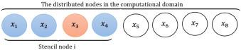
where is the number of nearest neighboring points on surrounding collocation point containing the collocation node itself. Fig. 1 shows the distributed nodes in the computational domain with a support domain.
The weighting coefficients at the support domain are the unknown coefficients to be calculated. The stencil weights arise by enforcing the linear constraint (5) within the space spanned through the RBF that are centered at stencil node locations, so that
This expression (6) can be simplified to
where
The weighting coefficients can be calculated from the aforesaid system. For non-singularity of the coefficient matrix in the system (7), we can refer to [44].
2.3. Discretization of the GPE
Here, we discretize spatial derivatives of the GPE by using the LRBF-FD method. For this aim, the first, second and third order derivatives of can be estimated with the help of the function values at a set of nodes (including ) in the support domain of . That is, we can write
where and the symbol represents the weighted differences at the support domain for the order derivatives The structure of matrices , and depends on the number of points in each support domain. For instance, if we choose three nodes in each support domain, then the matrices , and are tridiagonal matrices.
Inserting Eqs. (9), (10) and (11) in Eq. (1) and collocating the nodal points in it, we obtain semi-discrete system in the following system of ODEs:
Now, we use an ODE solver to solve the ODE system (12) in the temporal direction. We can implement for this aim, the ODE solver “command ode15s” that is acceptable for stiff ODEs and other traditional time-stepping methods. The method of lines constitutes an approach that utilizes FD in the temporal direction to determine the solution for the system of ODEs. Generally, this method may be considered stable provided each eigenvalue of the space discretization operator, scaled by using the temporal step (denoted by ), lies in the stability domain of the operator that discretizes time. In what follows, the Algorithm 1 illustrates the full discretization for the one dimensional nonlinear GPE.
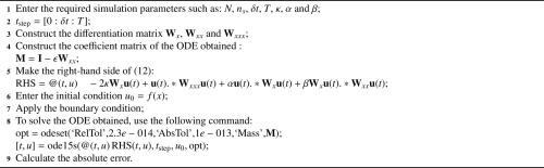
Algorithm 1. Full discretization of the GPE. |
3. Numerical results and discussion
The current section illustrates the simplicity, applicability and superiority of the proposed strategy by using two numerical examples on the GPE. We calculate the , , and norm errors in order to check the accuracy and adaptability of the LRBF-FD as:
where denotes the number of collocation nodes and and represent the exact and numerical solutions, respectively.
In the numerical illustrations, we apply the multiquadric (MQ) RBF as basis function with the shape parameter . Acceptable conditioning results need small shape parameters and large separation distances between the centers. Additionally, we apply the algorithm provided by Sarra [45] in this paper to calculate an optimal shape parameter (see Algorithm 2), where represents a coefficient matrix, “svd” denotes the singular value decomposition (SVD), and and are the largest and smallest singular values obtained from the SVD, respectively. In this algorithm, we choose , and All numerical simulations were performed by using MATLAB R2016a in a computer system having a configuration with memory 8.00G RAM. The time needed to obtain the solutions of the GPE is denoted by “CPUTime” in seconds and the condition number (CN) of the coefficient matrix is evaluated based on the MATLAB command condest.
Example 1 Let us consider the nonlinear GPE (1) on the space interval with the exact solution of the form and the following parameters in two cases
Case I ,
Case II ,
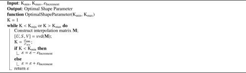
Algorithm 2. Optimal shape parameter [45]. |
This problem is examined by means of the LRBF-FD method with various parameters of , and at the final time . Table 1 lists the norm errors, CN and CPU run times (in seconds) for Case I with when at various values of stencil sizes . Table 2 compares the , , and norm errors and CPU run times with method described in Zabihi and Saffarian [19] for Case I by taking , and at several final times. Table 3 makes the comparison of the , , and norm errors and CPU run times with method introduced in Zabihi and Saffarian [19] for Case II by choosing , and at several final times. In view of Tables 2 and 3, we can see that the LRBF-FD collocation technique is more accurate than the scheme presented in Zabihi and Saffarian [19]. Fig. 2 plots the motion of the single solitary wave with and at different final times in Case I over spatial domain . Fig. 3 represents the motion of the single solitary wave with and at various final times in Case II over spatial domain . As seen in Figs. 2 and 3, the single solitons move to the left at a constant speed preserving their amplitude and shape. Fig. 4 portraits the soliton profiles in Case I when , and at various temporal intervals. Fig. 5 presents the soliton profiles in Case II by letting , and at various temporal intervals. Fig. 6 depicts the contour of solutions and associated absolute errors in Case I by taking , and at temporal interval [0,4]. Fig. 7 represents the contour of solutions and associated absolute errors in Case II by choosing , and at temporal interval [0,2]. Finally, Fig. 8 displays the sparsity patterns of the coefficient matrix for two different stencil sizes with
Example 2 We consider the nonlinear GPE (1) on the space interval with the exact solution of the form and the following parameters
Table 1. norm errors, CN and CPUTime of Example 1 for Case I with when at various stencil sizes . |
| CN | CPUTime | |||
| 400 | 113 | 2.341001 | ||
| 400 | 119 | |||
| 400 | 139 | |||
| 400 | 155 | |||
| 400 | 175 |
Table 2. , , and norm errors and CPUTime when , and at different final times in Case I over the spatial domain for Example 1. |
| Method [19] | LRBF-FD | ||||||
| CPUTime | |||||||
| 0.5 | 0.325940 | ||||||
| 1.0 | 0.423046 | ||||||
| 1.5 | 0.524313 | ||||||
| 2.0 | 0.631450 | ||||||
Table 3. , , and norm errors and CPUTime by considering , and at different final times in Case II over spatial domain for Example 1. |
| Method [19] | LRBF-FD | ||||||
| CPUTime | |||||||
| 1 | 0.295395 | ||||||
| 2 | 0.327970 | ||||||
| 3 | 0.357182 | ||||||
| 4 | 0.381461 | ||||||
| 5 | 0.406676 | ||||||
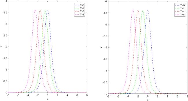
Fig. 2. Motion of the single solitary wave with and at different final times in Case I over spatial domain for Example 1. |
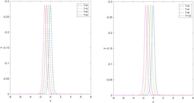
Fig. 3. Motion of the single solitary wave with and at various final times in Case II over spatial domain for Example 1. |
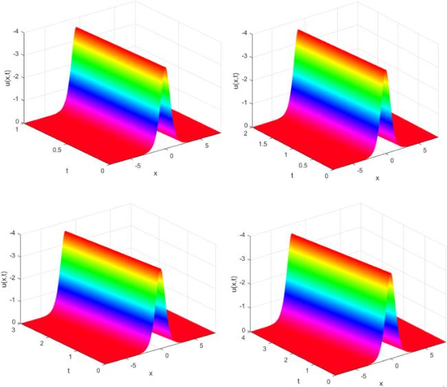
Fig. 4. The soliton profiles of the GPE when , and in Case I over spatial domain for Example 1. |
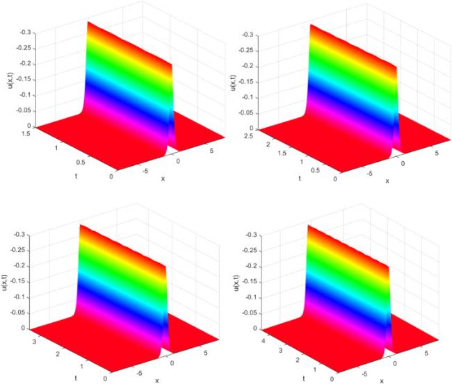
Fig. 5. The soliton profiles of the GPE with , and in Case II over spatial domain for Example 1. |
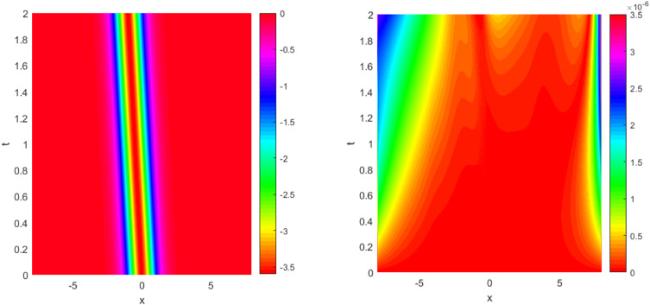
Fig. 6. The contour of solutions and associated absolute errors when , and in Case I over spatial domain for Example 1. |
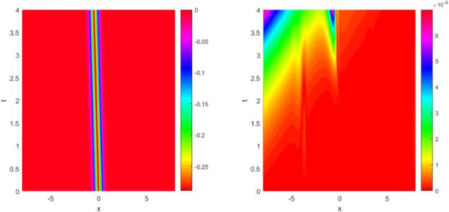
Fig. 7. The contour of solutions and associated absolute errors with , and in Case II over the spatial domain for Example 1. |
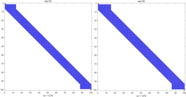
Fig. 8. The sparsity patterns of the coefficient matrix for two different stencil sizes with . |
Here, we simulate this example by using the LRBF-FD method with various parameters of , and at the final time . Due to the numerical solutions in this example are small, therefore, we use the relative error to show the effectiveness of the method as:
Table 4 reports the norm errors, CN and CPUTime with when for different values of stencil sizes . Table 5 compares the , , and norm errors and CPU run times with technique introduced in Zabihi and Saffarian [19] by letting , and at various values of final times. From Table 5, we can observe that the LRBF-FD collocation technique is more accurate than the method described in Zabihi and Saffarian [19]. Fig. 9 shows the soliton profiles with , and at various temporal intervals. Finally, Fig. 10 portraits the contour of solutions and associated absolute errors when , and at temporal interval [0,6].
Table 4. norm errors, CN and CPUTime of Example 1 with when for different stencil sizes. |
| CN | CPUTime | |||
| 800 | 191 | |||
| 800 | 219 | |||
| 800 | 299 | |||
| 800 | 609 | |||
| 800 | 685 |
Table 5. , , , and norm errors and CPUTime when , and at various final times over the spatial domain for Example 2. |
| Method [19] | LRBF-FD | ||||||||
| CPUTime | |||||||||
| 1 | 0.431546 | ||||||||
| 2 | 0.437426 | ||||||||
| 3 | 0.444489 | ||||||||
| 4 | 0.466018 | ||||||||
| 5 | 0.467160 | ||||||||
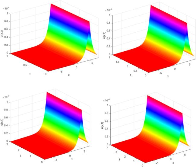
Fig. 9. The soliton profiles of the GPE when , and over the spatial domain in Example 2. |
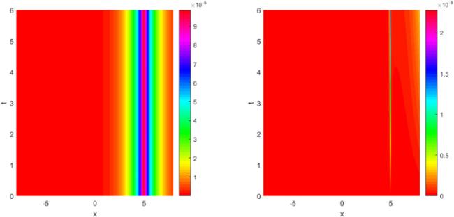
Fig. 10. The contour of solutions and associated absolute errors with , and over spatial domain in Example 2. |
4. Conclusions
This paper proposed an efficient and robust computational algorithm to simulate the one dimensional nonlinear GPE without using the linearization. The structure of the method involved two stages. First, the spatial dimension was approximated by virtue of the LRBF-FD collocation method. Second, the time dimension was discretized using the method of lines that yields a system of nonlinear ODEs. Furthermore, the obtained nonlinear system of ODEs was solved using an ODE solver to derive high-numerical results. The LRBF-FD collocation method efficiently handles the computational load unlike the case with the dense and ill-conditioned matrices required using global RBF collocation techniques. Two numerical examples demonstrated that the proposed method is efficient and accurate. The results obtained in this paper showed that the proposed method has great potential for simulating nonlinear evaluations.
Declaration of Competing Interest
Authors declare that they have no conflict of interest.
Acknowledgment
The authors are very grateful to the three anonymous referees for their valuable comments and suggestions that improved the original manuscript greatly. In addition, Anh Tuan Nguyen is supported by Van Lang University.
