
1. Introduction
The analysis of the physical phenomena in the sense of their mathematical modeling is an important tool in applied science and engineering. These models often can be described in the form of nonlinear partial differential equations (NLPDE) or a system of the same kind with the ability to better simulate these complex systems and their physical situations. Thus, finding accurate solutions to these types of equations capture the interest of many researchers driving them to investigate more in their studies for its solutions. The applicability of these models can be witnessed in many branches of science and engineering including fluid mechanics, nonlinear dynamics, quantum field theory, plasma physics, and solid-state physics. They have enjoyed an intense period over the past few years for numerical and theoretical points of view. One of these types of equations are the nonlinear evolution equations (NLEEs) which has tremendous applications in science. Moreover, studies of finding the soliton solutions to these types of equations attracted huge number of studies in the various fields [1], [2], [3], [4], [5], [6], [7], [8], [9].
Recently, fractional calculus has attracted the attention of many researchers with its ability to provide more realistic models of mathematical type for simulating application NLPDE [[10], [11], [12], [13], [14], [15], [16], [17]]. There has been tremendous research work which has been raised aiming for finding the solutions for these nonlinear fractional models including the classical case. Up until now, several methods have been adopted for solving these models including the Bäcklund transform method [18], Hirota bilinear method [19], inverse scattering method [20], Darboux transformation method [21], general projective Riccati equation method [22], sub-equation method [23], Kudryashov method [24], Jacobi elliptic method [25], modified extended tanh-expansion method [26], solitary wave ansatz method [27], and Riccati equations mapping method [28]. Each of these methods has its advantages and disadvantages which gives some of them the ability to provide better results than the other method in terms of accuracy and efficiency.
and it’s generalized form as:
where and are parameters. Furthermore, he used the Hereman-Nuseri approach to get the numerous soliton solutions for each model. The search for solitons of NLEEs has sparked a lot of attention in recent decades, because such a class of equations may describe a wide range of phenomena from science to engineering. Solitons are stable nonlinear localized solitary waves that preserve their shape while traveling at a constant velocity and may be classified as dark or bright depending on the governing models; they play an important part in many nonlinear physical phenomena. Soliton propagation has been utilized to explain several important oceanic phenomena, including nonlinear shallow and deep water wave propagation [29], [30], [31], [32], [33], [34], [35], [36], [37]. For instance, dark solitons have lately piqued curiosity in the context of surface gravity water waves: in two seminal studies conducted in water wave tanks, black and gray solitons were discovered on the surface of the water [30], [31].
where and are nonzero real parameters and ( ) is the fractional order. Therefore, in the study the conformable derivative (CD) will be explored. The fundamental reason for examining this sort of local derivative is that, when compared to other fractional derivative definitions, the CD can meet numerous properties spanning the chain, product, or quotient rules. To exact the dark solitons, singular solitons, periodic wave, and rational form solutions under certain parametric conditions, we employed two novel integrable techniques. These methods are the sub-equation and generalized Kudryashov methods which have been applied many times for solving strong nonlinear models in the field of applied sciences and engineering. The sub-equations method has been used to find soliton solution type different type of equations including space time-fractional equation [40], perturbed nonlinear Schrödinger [23], conformable fractional PDE [41], and others. Also, the generalized Kudryashov method have been used to solve other type of equations including fractional mathematical biology problems [42], coupled sine Gordon equations [43], fractional Boussinsque equations [44], fractional Klein Gordo equation [45], Cahn Hilliard equations [46], Kuramoto-Sivashinsky equation [47], many other equations that can be found in [48], [49], and references therein. It should be emphasized that the discovery of new models that incorporates soliton-type solutions are an intriguing outcome that will also aid future research in numerous fields of applied science and engineering.
The organization of the paper is as follows: In Section 2, we give some preliminaries regarding the fractional calculus that will be used in later sections. In Section 3, a summary for the two proposed methods is provided. Section 4 illustrates the main steps for solving Eqs. (3)–(6) using the two techniques and in Section 5 the results and graphical behavior for some obtained solutions are discussed. Finally, in Section 6 contains a conclusion for the study.
2. Preliminaries
In this section, we summarize some basic definitions, notations and theorems used in this present study.
If is -differentiable in some where and the exists, then by definition
1.
2.
3.
4.
5. is constant.
6. If is differentiable, then
Theorem 2.5 ([52]). Let be a differentiable and -differentiable function. Let be a differentiable function defined in the range of Then
Also, using the approach defined in [51] to obtained Definitions 2.3 and 2.4, we acquire the following:
Definition 2.6 Let be three times continuously differentiable and then
Definition 2.7 Let be three times continuously differentiable and then
We later use Definitions 2.6 and 2.7 and Mathematica software package to verify all obtained solutions by putting them back in their original equations.
3. Summary of the proposed methods
where indicates the conformable derivative. Through the use of the fractional wave transform [58]
we reduced Eq. (15) into a nonlinear ordinary differential equation (NODE) as:
where and are parameters that will be determined afterwards. The solutions of Eq. (17) can be presumed as:
where are the constants to also be calculated thereafter and is a positive integer to be found through balancing procedure [59] in Eq. (17). A summary of the two proposed integrable method will be discuss in the following subsections. In the following subsections, a quick summary of the two suggested integrable methods will be discussed.
3.1. Sub-equation method (SEM)
The function in Eq. (18) satisfy the Riccati equation
where is a random constant. The solutions of Eq. (19) are listed as:
By inserting Eqs. (18) and (19) into Eq. (17), we obtain some polynomials in Setting all the coefficients of to zero gives system of equations. Solving this system and plugging the obtain parameters into Eq. (18), with the use of Eq. (20), we achieved the desired exact solutions for Eq. (15) instantly.
3.2. Modified Kudryashov method (MKM)
In Eq. (18), the function satisfies the ODE
and the solution of Eq. (21) is given by
where and is the constant integration. Again, by substituting Eqs. (18) and (21) into Eq. (17), we get some polynomials in Set all coefficients to the zero yield algebraic equations. Solving this algebraic system of equations. Furthermore, inserting the obtain constants into Eq. (18), assisted by Eq. (22), we obtain the required exact solutions for Eq. (15).
4. Application of the proposed method
In this section, we apply the modified Kudryashov and sub-equation methods in the conformable sense to examine various types of new generalized fifth order nonlinear equations.
4.1. The first extended fifth-order nonlinear equation
Consider Eq. (3) given by
Using the wave transformation we reduces Eq. (23) to
SEM: Putting Eq. (25) into Eq. (24) assisted by Eq. (19), then letting the coefficients of to zeros, yields the below equations:
The above solvable system results to
Using Eq. (25), together with Eqs. (27) and (20), we get the traveling-wave solutions as follows:
MKM: Putting Eq. (25) into Eq. (24) assisted by Eq. (21), then letting the coefficients of to zeros, yields the below equations:
The above solvable system results to
Using Eq. (25), together with Eqs. (30) and (22), we get the traveling-wave solutions as follows:
4.2. The second extended fifth-order nonlinear equation
Consider Eq. (4) given by
Employing we transform the above equation to
Balancing with we obtain Thus, from Eq. (18) we obtain
SEM: Substituting Eq. (34) into Eq. (33) assisted by Eq. (19), then setting the coefficients of to zeros, yields the below set of simultaneous algebraic equations:
The above solvable system results to
Using Eq. (35), together with Eqs. (37) and (20), we get the traveling-wave solutions as follows:
MKM: Putting Eq. (34) into Eq. (33) assisted by Eq. (21), then letting the coefficients of to zeros, yields the below equations:
The above solvable system results to
Using Eq. (34), together with Eqs. (39) and (22), we get the traveling-wave solutions as follows:
4.3. The third extended fifth-order nonlinear equation
Consider Eq. (5) given by
Employing we transform the above equation to
Balancing with we obtain Thus, from Eq. (18) we obtain
SEM: Substituting Eq. (43) into Eq. (42) assisted by Eq. (19), then setting the coefficients of to zeros, yields the below set of simultaneous algebraic equations:
The above solvable system results to
Using Eq. (44), together with Eqs. (45) and (20), we get the traveling-wave solutions as follows:
MKM: Putting Eq. (43) into Eq. (42) assisted by Eq. (21), then letting the coefficients of to zeros, yields the below equations:
The above solvable system results to
Using Eq. (43), together with Eqs. (48) and (22), we get the traveling-wave solutions as follows:
4.4. The fourth extended fifth-order nonlinear equation
Consider Eq. (6) given by
Employing we transform the above equation to
Balancing with we obtain Thus, from Eq. (18) we obtain
SEM: Substituting Eq. (52) into Eq. (42) assisted by Eq. (19), then setting the coefficients of to zeros, yields the below set of simultaneous algebraic equations:
The above solvable system results to
Using Eq. (53), together with Eqs. (45) and (20), we get the traveling-wave solutions as follows:
MKM: Putting Eq. (52) into Eq. (51) assisted by Eq. (21), then letting the coefficients of to zeros, yields the below equations:
The above solvable system results to
Using Eq. (52), together with Eqs. (57) and (22), we get the traveling-wave solutions as follows:
5. Graphical representation and discussion
The graphical depiction of some solutions are shown in this section to demonstrate their features. In particular, the two dimensional (2D), three dimensional (3D), and the contour plots of Eqs. (28) and (30). Figure 1 shows the 3D, 2D, and contour plots of a dark soliton solution in Eq. (28) with the following parameters; and In Fig. 2, we presented the 3D, 2D, and contour plots of a singular soliton solution in Eq. (28) with and Figure 3 depicted the 3D, 2D, and contour plots of a perodic solution in Eq. (28) with and . Also, in Fig. 4, we shown another form of dark soliton using the solution in Eq. (30) with and . The 2D plots for different fractional order ( ) are illustrated in Figs. 1(c), 2(c), 3(c), and 4(c) respectively.

Fig. 1. The plots of (Eq. (28)) in (a)&(b) and (c) with different |

Fig. 2. The plots of (Eq. (28)) in (a)&(b) and (c) with different |
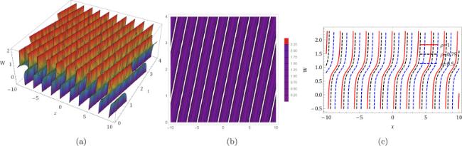
Fig. 3. The plots of (Eq. (28)) in (a)&(b) and (c) with different |
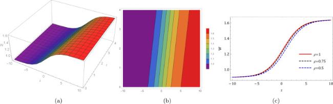
Fig. 4. The plots of (Eq. (30)) in (a)&(b) and (c) with different |
6. Conclusion
In this study, two effective techniques, namely, the sub-equation and generalized Kudryashov methods are employed to acquired soliton type solutions of four new conformable fractional nonlinear evolution equations. Under specific parametric conditions, the solutions acquired are dark solitons, singular solitons, a periodic wave, and rational solutions. The main steps for these methods are illustrated and then used for solving four forms of the nonlinear equations. The results obtained from applying these methods prove that these method are promising for solving fractional differential equations. A graphical representation of the solutions is provided for different values of obtained parameters. From these figures, the obtained solutions have the solitons like behavior and may illustrate some physical phenomena in various fields of applied science and engineering. In the future, we hope to employ various approaches to investigate these four generalized nonlinear fractional fifth-order equations and acquire their breather, lump, and soliton solutions.
Declaration of Competing Interest
The authors declare that they have no known competing financial interests or personal relationships that could have appeared to influence the work reported in this paper.
