
1. Introduction
The seminal work of Leibniz and the L’Hôpital contributed immensely to the advancement of the basic idea of fractional calculus [1], [2], [3]. The beauty of fractional calculus is its ability to accurately capture the exact behavior of many complex fractional models in science, engineering, and finance [4], [5], [6], [7], [8], [9], [10], [11], [12], [13], [14], [15]. The concept of fractional calculus is believed to be a generalization of integer order calculus [16], [17], [18], [19], [20], [21], [22], [23], [24], [25]. For the most recent related works on fractional calculus, the readers may to refer to [26], [27], [28], [29], [30], [31], [32], [33], [34], [35]. The previous work of Kuramoto and Sivashinsky [36], [37], [38], [39] on the fourth-order nonlinear partial differential equation which provided the general idea on the GKSE also known as the Generalized Kuramato-Sivashinky equation exhibited a chaotic behavior with non-zero constants ( ) of the form
The GKSE was used to model important applications in science and engineering such as the chemical reaction dynamics, the flows in pipes and at interfaces, the flame propagation and reaction-diffusion systems. In the field of ocean engineering, the GKSE arises naturally in various applications such as the viscous flow problems, the magneto hydrodynamics, the weather forecasting and the climate modelling, the turbulence in micro-tides, the offshore industry, and so on. The GKSE provides solution to the most of the none-linear differential equations that exhibit chaotic behavior and is considered as a prototype to the larger class of the well-known Burger’s equations. If and , the generalized Kuramoto-Sivashinky Eq. (1) reduces to Kuramoto-Sivashinky equation (KSE) [40]. Shah et al. solved Eq. (1) using the Laplace transformation and the variational iteration method [41]. In 2019, Taneco-Hernandez et al. obtained the analytical solutions of the KSE via the homotopy perturbation transform method [42]. In [43], the modified Kudrayshov method was applied to Eq. (1) when . Kurulay et al. used the well-known homotopy analysis method to analyzed the analytical solutions of the GKSE [44]. Using the B-spline function, the numerical solutions of Eq. (1) when and [45] was illustrated. In 2018, Rosa et al. derive the classical symmetries and the low-order conservation laws of the GKSE [46]. Veeresha and Prakasha applied the q-homotopy analysis transform method to obtained the analytical solutions of the KSE [47]. Xu and Shu utilized the local discontinuous Galerkin techniques to analyzed the numerical solution of the KSE [48]. In 2011, Porshokouhi and Ghanbari solved the KSE via the variational iteration technique [49]. Khater and Temsah applied the Chebyshev spectral collocation techniques on KSE [50]. In [51], Ye et al. obtained the numerical solutions of the KSE via Lattice Boltzmann model. In 2015, Sahoo and Ray obtained a new exact solutions of the KSE [52]. For more numerical solutions of the GKSE, the readers are refereed to [53], [54], [55], [56], [57].
The aim of this work is to proposed an analytical technique called the homotopy analysis -transform method (HAJTM) via the Caputo (C) [58], [59], the Caputo-Fabrizio (CF) [60], and the Atangana-Baleanu (AB) fractional derivatives [61] for solving the non-integer generalized Kuramato-Sivashinky equation. The HAJTM is a combination of the well-known homotopy analysis method which was first proposed by Liao [62], [63] and the -transform method which is a modification of the well-known Sumudu integral transform and the natural transform method [64]. The -transform was first introduced by Maitama and Zhao in 2020, and was successfully utilized to solved problems which cannot be solved by the natural transform and the Sumudu integral transform [65]. The -transform converges to Laplace transform when the variable . In [66], the -transform was applied to solved differential equations with variable coefficient which cannot be solve using the well-known Laplace transform. The advantages and disadvantages of the proposed HAJTM are as follows:
•The HAJTM can be applied to analyzed the solution of linear or nonlinear fractional models in ocean engineering without any restrictive assumptions.
•The proposed method gives a series solutions which converges rapidly within few iterations.
•The most important aspect of the suggested method is the existence of the non-zero convergence control parameter which is used to adjust and control the convergence of the series solutions.
•The HAJTM is used to investigate the analytical and numerical solutions of the fractional generalized Kuramato-Sivashinky equation which naturally arises in oceanic engineering.
•The HAJTM can only be applied to fractional models with boundary or initial conditions.
The work is organized as follows: In Section 2, definitions pertaining -transform, fractional derivative with non-singular kernel, and some important theorems used in this paper are presented. In Section 3, the fractional generalized Kuramato-Sivashinky equation is examined via the Atangana-Baleanu fractional derivative. In Section 4, an iterative method via the Caputo, the Caputo-Fabrizio, and the Atangana-Baleanu fractional derivatives is given. In Section 5, the applications of the HAJTM to fractional generalized Kuramato-Sivashinky equation via the three fractional derivatives are illustrated. In Section 6, which is the last part of this paper, the concluding remarks are presented.
2. Preliminaries
In this section, we present the basic definition of the fractional derivative with non-singular kernel known as the Atangana-Baleanu fractional derivative. Moreover, the -transform and some of its useful theorems used in this paper are also presented.
Definition 1 [61] Let and not necessarily differentiable, then the Atangana-Baleanu fractional derivative in Riemann-Liouville sense is defined as
where is a normalization function with property
Definition 2 [61] Let , then the Atangana-Baleanu fractional derivative in Caputo sense is defined as
where is a normalization function having the property
Definition 3 [14] The associative fractional integral related to the AB fractional derivative is defined as
where satisfies
Theorem 2 The -transform of Caputo fractional derivative is defined as
where
Proof Thanks to Caputo fractional derivative [59] which help us to get
where
is the Euler-Gamma function.
where
is the Euler-Gamma function.
The proof ends. □
Theorem 3 Let , then the -transform of the Caputo-Fabrizio fractional derivative is defined as
where satisfies
Applying the convolution property of -transform, gives
This completes the proof. □
Theorem 4 The -transform of the Atangana-Baleanu fractional derivative is given by
where satisfies
Applying the convolution property of -transform, we get
This completes the proof. □
In the following section, we present the new fractional generalized Kuramoto-Sivashinky equation using the AB fractional derivative.
3. Modelling fractional generalized Kuramoto-Sivashinky equation with Atangana-Baleanu fractional derivative
In this section, we study the fractional model of generalized Kuramoto-Sivashinky equation via the AB fractional operator
where
Applying the AB fractional derivative operator on Eq. (12), we get
For clarity, we adopt the following simple notation
Then Eq. (13) becomes
In Eq. (15), the kernel satisfies the Lipschitz condition provided the function is has an upper bound. Thus, if the function has an upper bound then
With the help of triangular inequality of the norm we arrive at
where .
In Eq. (17), the functions and are bounded. This implies and , where are constants. Thus, setting , we get
Hence, the kernel satisfies the Lipschitz condition.
Theorem 5 Let the function be bounded, then the operator
satisfies the Lipschitz condition.
Proof Without loss of generality. Let assume the functions and are bounded with initials , then we get
where .
This completes the proof. □
Theorem 6 If the function is bounded, then the operator denoted as
satisfies the following result
where represent the inner product of function with the differentiation restricted in .
Proof Let the functions be bounded, then we have
where
The proof is completed. □
Theorem 7 Suppose the function is bounded, then the operator defined in Eq. (21) satisfies
Proof Let and the functions be bounded, then we have
where
This completes the proof. □
3.1. The existence and uniqueness analysis of the FGKSE
In this section we prove the existence and uniqueness of the fractional generalized Kuramoto-Sivashinky equation using the AB fractional derivative. Based on Eq. (15), we formulate the following iterative scheme
with initial
Moreover, the algebraic difference of the successive terms is given by
At this stage, it is crucial to know that
Then by virtue of Eq. (28), we deduce
Computing the triangular inequality of Eq. (30), yields
Since the kernel satisfies the Lipschiz condition, then
or
From Eqs. (30) to (33), we obtain the following useful theorem
Theorem 8 The model of fractional generalized Kuramoto-Sivashinky equation given in Eq. (12) has solution which satisfies the following inequality
Proof Let the function be bounded. Besides, the kernel satisfies Lipschitz condition. By virtue of Eq. (33) and the iteration scheme, we arrive at
Thus,
exist. The result of Eq. (36) is the solution of Eq. (12), to verify that we consider
Then,
Besides, following the same fashion we recursively obtain
At the moment, setting , we get
Finally, computing the limit of Eq. (40) as , yields
This completes the proof of the existence. □
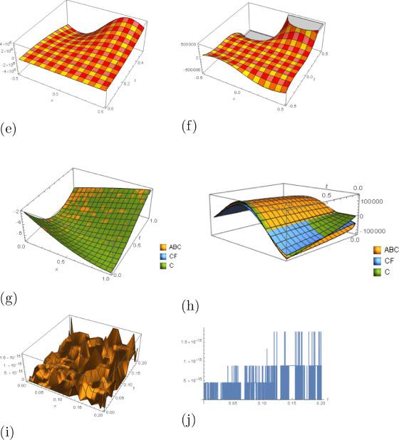
Fig. 1. Comparison of the analytical and numerical solutions of the FGKS Eq. (77) using the Caputo fractional derivative for different and . |
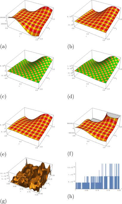
Fig. 2. Comparison of the analytical and numerical solutions of the FGKS Eq. (78) using the Caputo-Fabrizio fractional derivative for different and . |
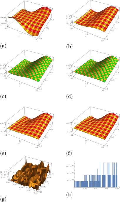
Fig. 3. Comparison of the analytical and numerical solutions of the FGKS Eq. (79) using the Atangana-Baleanu fractional derivative for different and . |
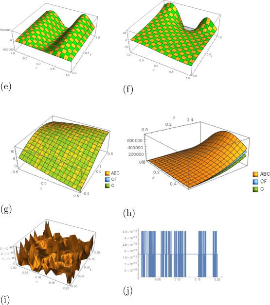
Fig. 4. Comparison of the analytical and numerical solutions of the FGKS Eq. (92) using the Caputo fractional derivative for different and . |
It now remain to show the uniqueness of solution for fractional generalized Kuramoto-Sivashinky equation with the Atangana-Baleanu fractional derivative.
Without loss of generality, let claims there exist another solution for the model on Eq. (12), then their successive difference is given by
Computing the norm on Eq. (42), we deduce
Recall that the kernel already satisfies the Lipschitz condition, then
The inequality of Eq. (44) yields
As a direct consequence of inequality Eq. (45) above, we obtain the following theorem
Theorem 9 The fractional generalized Kuramoto-Sivashinky Eq. (12) possesses a unique solution if the following inequality is satisfied
Proof Since the kernel of inequality Eq. (14) satisfies Lipschitz condition, and the aforementioned requirement, then
Thus
This implies
This completes the proof. □
In the next section, we introduce the new homotopy analysis -transform method for solving nonlinear fractional generalized Kuramato-Sivashinky equation.
4. The homotopy analysis -transform method via the Caputo, the Caputo-Fabrizio, and the Atangana-Baleanu fractional derivatives
Consider the following nonlinear fractional generalized Kuramoto-Sivashinky equations
Where is the Caputo, the Caputo-Fabrizio, and the Atangana-Baleanu fractional derivatives and
Computing the -transform of the Caputo, the Caputo-Fabrizio, and the Atangana-Baleanu fractional derivative on Eqs. (50) to (52), we arrive at
respectively.
Upon simplifying Eqs. (53) to (55), we get
where
and
and
The required nonlinear operator is defined as
where is a nonzero auxiliary parameter, is a real-valued function of , and is to be replaced by (C), (CFC), and (ABC) respectively. We defines 0th-order homotopy of the form
where is the -transform, is the embedding parameter, (auxiliary function), (convergence control parameter), is the initial guess of , and is the unknown function.
Interestingly, the HAJTM provide us with the great chance to select the auxiliary parameter and the initial guess. Setting , in Eq. (58) gives the following result
When rises from 0 to 1, the solution moves from the initial guess to to the solution . Then applying the Taylor series expansion of with respect to we get
where
Besides, if , the auxiliary function , the initial guess, are selected properly, Eq. (58) converges at , and
is the solution of Eqs. (50) to (52). Moreover, based on Eq. (60), the governing equation can be deduced from the 0th-order deformation Eq. (58).
Define the vectors
Dividing Eq. (58) by after -times differentiation with respect to , and setting we get the th-order deformation equation
where
and
Operating the inverse -transform on both sides of Eq. (64) yields
Based on Eqs. (50) to (52), the is define as
Using Eq. (67), we solve for and get
where the superscript is to be substituted by the (C), the (CF), and the (ABC) respectively.
In the next theorem, we study the convergence analysis of the original problems Eqs. (50) to (52).
Theorem 10 Convergence analysis. As , , which is computed via Eq. (67) with help of Eq. (68) . Then it must be closed solution of Eqs. (50) to (52).
Proof Considering
Since , Then .
With the help of Eqs. (67) and (68), we arrive at
Considering , and the linearity property of Eq. (58), we have
Considering , and the linearity property of Eq. (58), we have
With the help of Eq. (68), we finally get
□
Where is to be replace by the Caputo, the Caputo-Fabrizio, and the Atangana-Baleanu fractional derivatives. Thus, Eq. (72) proved that is the closed solution of Eqs. (50), (51), and (52) respectively. □
Theorem 11 Let and be in Banach space . Then the HAJTM series solutions defined by Eq. (67) converges to the solution of Eqs. (50) to (52) provided .
Proof Considering the sequence of partial sum of the form
We are interested to prove that is a Cauchy sequence in . From the last hypothesis of the theorem, we have then
We are interested to prove that is a Cauchy sequence in . From the last hypothesis of the theorem, we have then
For any , we have
Then
since . Thus, we produces the required result. □ □
Theorem 12 Error analysis. Suppose and be its truncated solution. Let such that , , for , then
Proof Since , then
We obtain the required result. □
We obtain the required result. □
The analytical and the numerical solutions of the fractional GKSE are illustrated in the following section.
5. Applications
Example 1 Consider Eqs. (50) to (52), where
with the initial condition
Applying the -transform of the Caputo, the Caputo-Fabrizio, and the Atangana-Baleanu fractional derivative on Eqs. (77), (78), and (79) we get
respectively.
Simplifying Eqs. (81) to (83), gives
where
and
and
We defined the nonlinear operator as
Now the 0th-order deformation equation is
Multiplying Eq. (86) with after -times differentiation with respect to , and setting , we get the higher order ( th) deformation equation as
where
Inverting Eq. (87), we get
Upon solving Eq. (89) with , we get the following approximations
and so on.
Using the same procedure we obtain the remaining terms. Thus, the approximate solution of Eqs. (77), (78), and (79) using the proposed HAJTM are given by
As the exact solution of Eqs. (77) to (79) is given by
where and .
Example 2 Consider Eqs. (50) to (52), where
with the initial condition
Computing the -transform of the Caputo, the Caputo-Fabrizio, and the Atangana-Baleanu fractional derivative on Eqs. (92), (93), and (94) we get
respectively.
Table 1. Comparison of the numerical solutions of Eqs. (77) to (79) using the HAJTM and the LVIM [41] at and different time intervals. |
| HAJTM | LVIM [41] HAJTM | HAJTM | HAJTM | ||||
| Exact solutions | ABC | CFC | C | ||||
| 0.1 | 1.36131 | 1.31202 | 1.31402 | 1.31273 | 1.31455 | 1.31377 | 1.31532 |
| 0.2 | 1.39338 | 1.31089 | 1.31065 | 1.31122 | 1.31111 | 1.30952 | 1.31063 |
| 0.3 | 1.41971 | 1.31065 | 1.30856 | 1.31035 | 1.30874 | 1.30736 | 1.30755 |
| 0.4 | 1.44131 | 1.31101 | 1.30754 | 1.31004 | 1.30734 | 1.30668 | 1.30583 |
| 0.5 | 1.45903 | 1.31178 | 1.30742 | 1.31022 | 1.30683 | 1.30711 | 1.30527 |
| 0.6 | 1.47356 | 1.31284 | 1.30806 | 1.31083 | 1.30711 | 1.30838 | 1.30569 |
| 0.7 | 1.48547 | 1.31407 | 1.30933 | 1.3118 | 1.30808 | 1.31029 | 1.30696 |
| 0.8 | 1.49523 | 1.31539 | 1.31112 | 1.31307 | 1.30964 | 1.31266 | 1.30893 |
| 0.9 | 1.50323 | 1.3167 | 1.31332 | 1.31455 | 1.3117 | 1.31533 | 1.31147 |
| 1 | 1.50978 | 1.31794 | 1.31582 | 1.31619 | 1.31418 | 1.31817 | 1.31445 |
Table 2. Comparison of the numerical simulations of Eqs. (92) to (94) using the HAJTM and the LVIM [41], at and different time intervals. |
| HAJTM | LVIM [41] HAJTM | HAJTM | HAJTM | ||||
| Exact solutions | ABC | CFC | C | ||||
| 0.1 | -3.9996 | -4.74491 | -4.08462 | -4.47938 | -4.06525 | -4.02729 | -4.00794 |
| 0.2 | -3.9994 | -5.61008 | -4.29293 | -4.99779 | -4.22522 | -4.1884 | -4.07518 |
| 0.3 | -3.99911 | -6.7831 | -4.67612 | -5.72863 | -4.52608 | -4.56248 | -4.26213 |
| 0.4 | -3.99867 | -8.28573 | -5.27878 | -6.70216 | -5.01007 | -5.20899 | -4.62403 |
| 0.5 | -3.99802 | -10.1381 | -6.14383 | -7.94862 | -5.71942 | -6.17822 | -5.21314 |
| 0.6 | -3.99705 | -12.3593 | -7.31289 | -9.49826 | -6.69634 | -7.51478 | -6.07971 |
| 0.7 | -3.99562 | -14.9676 | -8.82653 | -11.3813 | -7.98308 | -9.25925 | -7.27238 |
| 0.8 | -3.99349 | -17.9806 | -10.7244 | -13.6281 | -9.62186 | -11.4492 | -8.8386 |
| 0.9 | -3.99034 | -21.4152 | -13.0456 | -16.2687 | -11.6549 | -14.1197 | -10.8248 |
| 1 | -3.98567 | -25.2879 | -15.8282 | -19.3335 | -14.1244 | -17.3039 | -13.2763 |
After simplifying Eqs. (96) to (98), we get
where
and
and
We defined the nonlinear operator as
The 0th-order deformation equation is
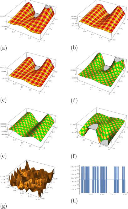
Fig. 5. Comparison of the analytical and numerical solutions of the FGKS Eq. (93) using the Caputo-Fabrizio fractional derivative for different and . |
Multiplying Eq. (101) with after -times differentiation with respect to , and setting , we get the higher order ( th) deformation equation as
where
Inverting Eq. (102), we get
Upon solving Eq. (104) with , we get the following approximations
and so on.
and so on.
Using the same procedure we obtain the remaining terms. Thus, the approximate solution of (93), (93), and (94) using the proposed HAJTM are given by
As the exact solution of Eqs. (92) to (94) is given by
5.1. Results and discussion
We discuss the analytical and numerical simulations of the fractional generalized Kuramoto-Sivashinky equation via the Atangana-Baleanu (AB), the Caputo-Fabrizio (CF), and the Caputo (C) fractional derivatives respectively. Figs. 1 to 6, show the result of the fractional GKSE obtained via none-singular kernel exhibits a new features or characteristic compared to the well-known Caputo fractional derivative. Moreover, the results of the Atangana-Baleanu fractional derivative is in excellent agreement with the Caputo fractional derivative. In Fig. 1(a) to (h), we plot the graphical solution behavior of Eq. (77) for different values of at different time interval in the Caputo sense. When and , the graphical solutions of Eq. (77) are presented in Fig. 1(a) and (b) respectively. The solutions of the fractional FGKSE for and are given in Fig. 1(c) and (d) respectively. In Fig. 1(e) and (f), the graphical solutions of the FGKS Eq. (77) is depicted for . Besides, the exact solutions of Eqs. (77) to (79) were compared in Fig. 1(g). In Fig. 1(h), the approximate solutions of Eqs. (77) to (79) are compared when and at different time intervals. The 3D error analysis of the FGKS is presented in Fig. 1(i). The 2D error estimate of the FGKS Eq. (77) is provided in Fig. 1(j). Moreover, we observe that the increase in the values of result in the increase in the turbulence behavior and vice-versa. The numerical simulations behavior of Eqs. (77) to (79) at and different values of were computed in Table 1, and the obtained results are in excellent agreement with all the three fractional derivatives and the LVIM [41].
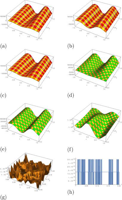
Fig. 6. Comparison of the analytical and numerical solutions of the FGKS Eq. (94) using the Atangana-Baleanu fractional derivative for different and . |
Using the Caputo-Fabrizio fractional derivative, in Fig. 2(a) to (h) we provided the graphical solutions of Eq. (78). For different values of and different time intervals, in Fig. 2(a) and (b) the graphical solutions of Eq. (78) are depicted when and . The graphical solutions of Eq. (78) are presented in Fig. 2(b) and Fig. 1(c) for and respectively. The surface solutions behavior of the FGKS Eq. (78) when are provided in Fig. 2(e) and (f). The 3D error analysis of the FGKS is presented in Fig. 2(g). The 2D error estimate of the FGKSE is plotted in Fig. 2(h). It is worth noting that the increase in the value of is directly proportional to increase in the chaotic behavior and vice-versa.
In Fig. 3(a) to (h), we depict the graphical solution behavior of Eq. (79) for different values of at different time intervals using Atangana-Baleanu fractional derivative. When and , the graphical solutions of Eq. (79) are provided in Fig. 3(a) and (b) respectively. The numerical solutions of the FGKSE for and are presented in Fig. 3(c) and (d). In Fig. 3(e) and (f), the analytical solution behavior of the FGKS Eq. (79) is depicted for . It is noticeable that the increase in the values of result in the increase in the chaotic behavior and vice-versa. The 3D error analysis of the FGKS Eq. (79) is presented in Fig. 3(g). The 2D error estimate of the FGKSE is plotted in Fig. 3(h).
In Fig. 4(a) to (h), the graphical solutions of Eq. (92) are computed using the Caputo fractional derivative. When and , the graphical solutions behavior of Eq. (92) are provided in Fig. 4(a) and (b) respectively. In Fig. 4(c) and (d), we Plotted the graphical solutions of the FGKSE for . In Fig. 4(e) and (f), the solutions of the FGKS Eq. (92) are provided for . Besides, we observe that the increase in the values of result in the increase in the turbulence behavior and vice-versa. Fig. 4(g) shows the result obtain by comparing the exact solutions of Eqs. (92) to (94). Also, the approximate solutions of Eqs. (92) to (94) were obtained in Fig. 4(h) with and at different time. The 3D error analysis of the FGKS Eq. (92) is presented in Fig. 4(i). The 2D error estimate of the FGKS Eq. (92) is presented in Fig. 4(j). The numerical simulations of Eqs. (92) to (94) at , , and different time intervals were computed in Table 2, and the obtained results are in excellent agreement with all the three fractional derivatives and the LVIM [41].
Using the fractional derivative with non-singular kernel the CF, we depicted the graphical solutions behavior of Eq. (93) in Fig. 5(a) to (h). In Fig. 5(a) and (b), the graphical solutions behavior of Eq. (93) for different values of and are provided. When and , we plot the graphical solutions of Eq. (93) in Fig. 5(c) and (d) respectively. In Fig. 5(e) and (f), the surface solutions behavior of the FGKS Eq. (93) are given when . It is worth noting that the increase in the value of is directly proportional to increase in the chaotic behavior and vice-versa. The 3D error estimate of the FGKS Eq. (93) is presented in Fig. 5(g). The 2D error of Eq. (93) is plotted in Fig. 5(h).
In Fig. 6(a) to (h), we compute the graphical solution behavior of Eq. (94) for different values of at different time intervals using the Atangana-Baleanu fractional derivative. The graphical solutions behavior of Eq. (94) when and are provided in Fig. 6(a) and (b) respectively. In Fig. 6(c) and (d), the numerical solutions of the GKSE for and are presented. In Fig. 6(e) and (f), the analytical solution behavior of the FGKS Eq. (94) for are depicted. The 3D error analysis of the FGKS is presented in Fig. 6(g). The 2D error estimate of Eq. (94) is plotted in Fig. 6(h).
6. Conclusions
Using fractional derivatives with non-singular kernel-the CF and the AB operators, we proposed a new semi-analytical method called the homotopy analysis -transform method for solving fractional GKSE. The GKSE is considered as a large class of generalized Burger’s equation mimics the well-known Navier-Stokes equations of fluid motion-an important aspect of oceanography which covers a wide range of topics such as waves, geophysical fluid dynamics, the ocean currents, and the geology of the sea floor. Our proposed analytical method proved to be highly efficient and the non-zero convergence-control parameter was used to accelerate and adjust the convergence of the series solutions. We proved the existence and uniqueness of the fractional GKSE via fixed-point theorem. Furthermore, the error estimate and convergence of the method are established. Moreover, using Mathematica 12, the numerical and analytical solutions behaviors of the fractional GKSE at different values of and are presented. It is imperative to note that the analytical and numerical solutions obtained via the non-singular kernel fractional operators (CF and AB) are in mutual agreement with the well-known singular kernel operator (Caputo). Finally, in the future, we plan to apply the proposed HAJTM to explore the analytical and numerical solutions of other fractional models arising in ocean engineering and its related areas.
7. Funding
This work was partially supported by the National Natural Science Foundation of China (12071261, 11871068, and 11831010), the National Key R&D Program (2018YFA0703900).
Declaration of Competing Interest
We have no conflicts of interest to disclose.
