On the interaction phenomena to the nonlinear generalized Hietarinta-type equation

Usman Younas; T.A. Sulaiman; Jingli Ren; A. Yusuf

doi:10.1016/j.joes.2022.06.027

Journal of Ocean Engineering and Science >

2024 , Vol. 9 >Issue 1: 89 - 97

DOI: https://doi.org/10.1016/j.joes.2022.06.027

Research article

On the interaction phenomena to the nonlinear generalized Hietarinta-type equation

Usman Younas ^a ,
T.A. Sulaiman ^b^,^c ,
Jingli Ren ^,^a^,^* ,
A. Yusuf ^b^,^c

Expand

^a State Key Laboratory of Power Grid Environmental Protection/Henan Academy of Big Data, Zhengzhou University, Zhengzhou 450001, China
^b Faculty of Science, Federal University Dutse, Jigawa, Nigeria
^c Department of Computer Engineering, Biruni University Istanbul, Turkey

^* E-mail address: renjl@zzu.edu.cn (J. Ren).

Received date: 2022-05-30

Revised date: 2022-06-05

Accepted date: 2022-06-13

Online published: 2022-06-16

Fold

Abstract

In this paper, we describe the nonlinear behavior of a generalized fourth-order Hietarinta-type equation for dispersive waves in (2 + 1) dimension. The various wave formations are retrieved by using Hirota's bilinear method (HBM) and various test function perspectives. The Hirota method is a widely used and robust mathematical tool for finding soliton solutions of nonlinear partial differential equations (NLPDEs) in a variety of disciplines like mathematical physics, nonlinear dynamics, oceanography, engineering sciences, and others requires bilinearization of nonlinear PDEs. The different wave structures in the forms of new breather, lump-periodic, rogue waves, and two-wave solutions are recovered. In addition, the physical behavior of the acquired solutions is illustrated in three-dimensional, two-dimensional, density, and contour profiles by the assistance of suitable parameters. Based on the obtained results, we can assert that the employed methodology is straightforward, dynamic, highly efficient, and will serve as a valuable tool for discussing complex issues in a diversity of domains specifically ocean and coastal engineering. We have also made an important first step in understanding the structure and physical behavior of complex structures with our findings here. We believe this research is timely and relevant to a wide range of engineering modelers. The results obtained are useful for comprehending the fundamental scenarios of nonlinear sciences.

Key words： Hirota's bilinear method; Lump-periodic solutions; Breather waves; Rouge waves; Multi-waves

Cite this article

Usman Younas , T.A. Sulaiman , Jingli Ren , A. Yusuf . On the interaction phenomena to the nonlinear generalized Hietarinta-type equation[J]. Journal of Ocean Engineering and Science, 2024 , 9(1) : 89 -97 . DOI: 10.1016/j.joes.2022.06.027

1. Introduction

A variety of scientific fields have been studied since the beginning of time, including mathematical physics, optics, biology, chemistry, fluid dynamics, all of which have their own unique interpretations. Due to the complexity of these events, their causes, and their consequences, it took a long time for this interpretation to become well-established and hopeful before it could be put to use for human benefit. Discovering NLPDEs was a major breakthrough in the vast field of mathematics because it helped clear up the fog that had previously obscured human perception. The NLPDE’s exact and approximate solutions are extremely useful in a wide range of physical events.

The interest of scholars and researchers in computer programmes that automate tedious and repetitive mathematical operations is growing. NLPDEs are essential in a variety of logical domains such as material science, fluid mechanics and ocean engineering, optical fibers, geochemistry and geophysics, and many others, and nonlinear science is one of the most fascinating fields of study in the modern scientific era. Due to their emphasis on investigating structure of systems, scholars have laid great emphasis on analytically or precisely precise results [1], [2], [3], [4], [5], [6], [7], [8], [9], [10], [11], [12], [13], [14], [15].

Nonlinear scientific research is one of the most intriguing fields of study for educators in the modern era. As a result of their unwavering dedication to examining the actual aspects of frameworks, the primary objective of researchers has been to produce exact solutions. In order to find exact solutions to NPDEs, researchers have designed a variety of approaches and computational techniques. Each method is designed to help researchers find a particular sort of solution [16], [17], [18], [19], [20], [21], [22], [23], [24], [25], [26], [27], [28], [29], [30], [31], [32], [33], [34], [35]. Using lump solutions, linear and nonlinear PDEs can be solved. All directions decay uniformly, and this is called a ”lump solution.” Lumpy solutions are found in a variety of scientific fields, including optics, water waves, and plasma. Lump soliton has been extensively used to study integrable equations. If you’re looking for a unique type of solution that rationally localizes in all directions, lump solutions and their interactions are a great place to start [36], [37], [38], [39], [40], [41], [42], [43], [44], [45], [46]. Zakharov [47] and Craik and Adam [48] were, respectively, the first to discover these solutions.

Additionally, the names freak, rogue, or monster waves relate to waves with a tremendous amplitude that emerge suddenly on the sea surface (wave from nowhere). These waves are often preceded and/or followed by deep troughs (holes). As Lawton points out, unusual waves have been a part of maritime folklore for generations. Seafarers speak about water walls, holes in the sea, and many consecutive big waves (three sisters) that arise unexpectedly in otherwise benign weather. However, beginning in the 1970s of the previous century, oceanographers began to believe them. The oil and maritime sectors’ observations indicate that there is indeed something like to a true monster of the deep that devours ships and crew without compassion or warning. There are numerous definitions for such enormous waves. Frequently, the word extreme waves refers to the tail of a conventional statistical distribution of wave heights (usually a Rayleigh distribution), whereas the term freak waves refers to large-amplitude waves that occur more frequently than the background probability distribution would predict. Haver and Andersen have posed the question of what constitutes a freak wave: a rare manifestation of a common statistic or a typical manifestation of a rare population. Occasionally, the term freak waves refers to waves that are excessively high, asymmetrical, or steep. The amplitude requirement for freak waves is more accepted now: their height should surpass the significant wave height by 2-2.2 times. Various physical models of the rogue wave phenomenon have been carefully explored and numerous laboratory experiments undertaken during the last three decades. The primary objective of these investigations is to gain a better understanding of the physics underlying the appearance of enormous waves and their relationship to environmental conditions (wind and atmospheric pressure, bathymetry and current field), as well as to provide the design of freak waves required for engineering purposes [49].

Howevr, the aim of this piece of research is to discuss different shapes of the waves in the forms of breather waves, lump-periodic, rouge waves and two wave solutiobs. The under consideration model is generalized Hietarinta-type equation which is analyzed by usig using Hirota’s bilinear method.

The generalized Hietarinta-type equation [50] is described as:

(1)

\begin{matrix} α_{1} (6 u_{x} u_{x x} + u_{x x x x}) + α_{2} (3 u_{t} u_{t t} + 3 u_{x t} v_{t t} + u_{x t t t}) + γ_{1} u_{y t} + γ_{2} u_{x x} \\ + γ_{3} u_{x t} + γ_{4} u_{x y} + γ_{5} u_{y y} = 0, \end{matrix}

where,

u = u (x, y, t), v = v (x, y, t), v_{x} = u,

and

γ_{i}, 1 ⩽ i ⩽ 5, α_{1}, α_{2}

are generally arbitrary constants. Now, if we take

α_{1} = γ_{1} = γ_{2} = 0

, then the generalized Hietarinta-type Eq. (1) presents a reduced nonlinear equation:

(2)

\begin{matrix} α_{2} (3 u_{t} u_{t t} + 3 u_{x t} v_{t t} + u_{x t t t}) γ_{3} u_{x t} + γ_{4} u_{x y} + γ_{5} u_{y y} = 0 . \end{matrix}

Now, our focus is to analyze the Eq. (2) by applying the HBM and different test functions. For proceeding, we consider the following transformation

(3)

\begin{matrix} u (x, y, t) = 2 {(\ln f)}_{x}, \\ v (x, y, t) = 2 (\ln f) . \end{matrix}

On putting Eq. (3) into Eq. (2), we get the bilinear form as:

(4)

\begin{matrix} γ_{5} (f f_{y y} - f_{y}^{2}) + 3 α_{2} (f_{t t} f_{t x} - f_{t} f_{t t x}) - f_{x} (γ_{3} f_{t} + α_{2} f_{t t t}) \\ + f (α_{2} f_{t t t x} + γ_{3} f_{t x}) + γ_{4} (f f_{y x} - f_{x} f_{y}) = 0 . \end{matrix}

2. Interaction aspects

2.1. Breather-type waves

Consider

(5)

\begin{matrix} f (x, y, t) & = & \exp (- ρ_{1} (x + y + δ_{0} t)) + m_{1} \cos (ρ_{0} (x + y + σ_{0} t)) \\ + m_{2} \exp (ρ_{1} (x + y + δ_{0} t)) . \end{matrix}

On solving Eq. (5) and Eq. (4), and on taking exponential and trigonometric’ coefficients to zero, provides

Set-1:

(6)

\begin{matrix} γ_{3} = \frac{α_{2} (- 3 δ_{0}^{2} ρ_{1}^{2} σ_{0} - 3 δ_{0} ρ_{0}^{2} σ_{0}^{2} + δ_{0}^{3} ρ_{1}^{2} + ρ_{0}^{2} σ_{0}^{3})}{σ_{0} - δ_{0}}, \\ γ_{5} = \frac{2 α_{2} δ_{0}^{3} ρ_{1}^{2} σ_{0} + 2 α_{2} δ_{0} ρ_{0}^{2} σ_{0}^{3} + γ_{4} δ_{0} - γ_{4} σ_{0}}{σ_{0} - δ_{0}}, m_{2} = - \frac{m_{1}^{2} ρ_{0}^{2} σ_{0}}{4 δ_{0} ρ_{1}^{2}} . \end{matrix}

Putting the Eq. (6) in Eq. (5), yields

(7)

\begin{matrix} f (x, y, t) & = & - \frac{m_{1}^{2} ρ_{0}^{2} σ_{0} e^{ρ_{1} (δ_{0} t + x + y)}}{4 δ_{0} ρ_{1}^{2}} + m_{1} \cos (ρ_{0} (σ_{0} t + x + y)) \\ + e^{ρ_{1} (- (δ_{0} t + x + y))} . \end{matrix}

Consequently, on solving the Eq. (7) and Eq. (3), we get

(8)

u (x, y, t) = \frac{2 (- \frac{m_{1}^{2} ρ_{0}^{2} σ_{0} e^{ρ_{1} (δ_{0} t + x + y)}}{4 δ_{0} ρ_{1}} - m_{1} ρ_{0} \sin (ρ_{0} (σ_{0} t + x + y)) - ρ_{1} e^{ρ_{1} (- δ_{0} t - x - y)})}{- \frac{m_{1}^{2} ρ_{0}^{2} σ_{0} e^{ρ_{1} (δ_{0} t + x + y)}}{4 δ_{0} ρ_{1}^{2}} + m_{1} \cos (ρ_{0} (σ_{0} t + x + y)) + e^{ρ_{1} (- δ_{0} t - x - y)}} .

(9)

v (x, y, t) = 2 \log (- \frac{m_{1}^{2} ρ_{0}^{2} σ_{0} e^{ρ_{1} (δ_{0} t + x + y)}}{4 δ_{0} ρ_{1}^{2}} + m_{1} \cos (ρ_{0} (σ_{0} t + x + y)) + e^{ρ_{1} (- δ_{0} t - x - y)}) .

Set-2:

(10)

\begin{matrix} δ_{0} = - \frac{i ρ_{0} σ_{0}}{ρ_{1}}, γ_{3} = 4 α_{2} ρ_{0}^{2} σ_{0}^{2}, γ_{5} = - γ_{4} . \end{matrix}

On manipulating the Eq. (10) and Eq. (5), the following result is obtained

(11)

\begin{matrix} f (x, y, t) & = & m_{2} e^{ρ_{1} (- \frac{i ρ_{0} σ_{0} t}{ρ_{1}} + x + y)} + m_{1} \cos (ρ_{0} (σ_{0} t + x + y)) \\ + e^{- ρ_{1} (- \frac{i ρ_{0} σ_{0} t}{ρ_{1}} + x + y)} . \end{matrix}

Hence, Eq. (11) and Eq. (3) gives the solutions

(12)

u (x, y, t) = \frac{2 (m_{2} ρ_{1} e^{ρ_{1} (- \frac{i ρ_{0} σ_{0} t}{ρ_{1}} + x + y)} + m_{1} ρ_{0} (- \sin (ρ_{0} (σ_{0} t + x + y))) - ρ_{1} e^{- ρ_{1} (- \frac{i ρ_{0} σ_{0} t}{ρ_{1}} + x + y)})}{m_{2} e^{ρ_{1} (- \frac{i ρ_{0} σ_{0} t}{ρ_{1}} + x + y)} + m_{1} \cos (ρ_{0} (σ_{0} t + x + y)) + e^{- ρ_{1} (- \frac{i ρ_{0} σ_{0} t}{ρ_{1}} + x + y)}} .

(13)

\begin{matrix} v (x, y, t) & = & 2 \log (m_{2} e^{ρ_{1} (- \frac{i ρ_{0} σ_{0} t}{ρ_{1}} + x + y)} + m_{1} \cos (ρ_{0} (σ_{0} t + x + y)) \\ + e^{- ρ_{1} (- \frac{i ρ_{0} σ_{0} t}{ρ_{1}} + x + y)}) . \end{matrix}

Set-3:

(14)

\begin{matrix} δ_{0} = - \frac{m_{1}^{2} ρ_{0}^{2} σ_{0}}{4 m_{2} ρ_{1}^{2}}, \\ γ_{3} = - \frac{α_{2} ρ_{0}^{2} σ_{0}^{2} (m_{1}^{6} ρ_{0}^{4} + 12 m_{2} (m_{1}^{2} - 4 m_{2}) m_{1}^{2} ρ_{0}^{2} ρ_{1}^{2} - 64 m_{2}^{3} ρ_{1}^{4})}{16 m_{2}^{2} ρ_{1}^{2} (m_{1}^{2} ρ_{0}^{2} + 4 m_{2} ρ_{1}^{2})}, \\ γ_{5} = - γ_{4} - \frac{α_{1} σ_{0}^{3} (m_{1}^{6} ρ_{0}^{6} + 16 m_{1}^{2} m_{2}^{2} ρ_{1}^{2} ρ_{0}^{4})}{8 m_{2}^{2} ρ_{1}^{2} (m_{1}^{2} ρ_{0}^{2} + 4 m_{2} ρ_{1}^{2})} . \end{matrix}

On tackling the Eq. (14) and Eq. (5), we have

(15)

\begin{matrix} f (x, y, t) = \exp (- ρ_{1} (- \frac{m_{1}^{2} ρ_{0}^{2} σ_{0} t}{4 m_{2} ρ_{1}^{2}} + x + y)) + m_{2} \exp (ρ_{1} (- \frac{m_{1}^{2} ρ_{0}^{2} σ_{0} t}{4 m_{2} ρ_{1}^{2}} + x + y)) + m_{1} \cos (ρ_{0} (σ_{0} t + x + y)) . \end{matrix}

Thus, when Eq. (15) and Eq. (3) are combined, we get

(16)

\begin{matrix} u (x, y, t) = \frac{2 (- ρ_{1} \exp (- ρ_{1} (- \frac{m_{1}^{2} ρ_{0}^{2} σ_{0} t}{4 m_{2} ρ_{1}^{2}} + x + y)) + m_{2} ρ_{1} \exp (ρ_{1} (- \frac{m_{1}^{2} ρ_{0}^{2} σ_{0} t}{4 m_{2} ρ_{1}^{2}} + x + y)) + m_{1} ρ_{0} (- \sin (ρ_{0} (σ_{0} t + x + y))))}{\exp (- ρ_{1} (- \frac{m_{1}^{2} ρ_{0}^{2} σ_{0} t}{4 m_{2} ρ_{1}^{2}} + x + y)) + m_{2} \exp (ρ_{1} (- \frac{m_{1}^{2} ρ_{0}^{2} σ_{0} t}{4 m_{2} ρ_{1}^{2}} + x + y)) + m_{1} \cos (ρ_{0} (σ_{0} t + x + y))} . \end{matrix}

(17)

\begin{matrix} v (x, y, t) = 2 \log (\exp (- ρ_{1} (- \frac{m_{1}^{2} ρ_{0}^{2} σ_{0} t}{4 m_{2} ρ_{1}^{2}} + x + y)) + m_{2} \exp (ρ_{1} (- \frac{m_{1}^{2} ρ_{0}^{2} σ_{0} t}{4 m_{2} ρ_{1}^{2}} + x + y)) + m_{1} \cos (ρ_{0} (σ_{0} t + x + y))) . \end{matrix}

•

Graphical view

The obtained results are depicted in the graphs below:

2.2. Lump-periodic solutions

In this section, we discuss the lump-periodic solutions on considering the following test function

(18)

\begin{matrix} f (x, y, t) = q_{1} \cosh (b_{1} x + b_{2} y + b_{3} t) + q_{2} \cos (b_{4} x + b_{5} y + b_{6} t) + + q_{3} \cosh (b_{7} x + b_{8} y + b_{9} t) . \end{matrix}

Switching Eq. (18) into Eq. (4), provides a polynomial in the terms of hyperbolic and trigonometric functions. Taking the same power coefficients, and equating each summations to zero, produces an algebraic system of equations, we obtain

Set-1:

(19)

\begin{matrix} b_{3} = - \frac{b_{4}^{2 / 3} {(b_{2} b_{4} - b_{1} b_{5})}^{2 / 3} \sqrt[3]{γ_{5}}}{\sqrt[3]{3} \sqrt[3]{α_{2} b_{1} {(b_{1}^{2} + b_{4}^{2})}^{2}}}, b_{6} = \frac{b_{1} {(b_{2} b_{4} - b_{1} b_{5})}^{2 / 3} \sqrt[3]{γ_{5}}}{\sqrt[3]{3} \sqrt[3]{b_{4}} \sqrt[3]{α_{2} b_{1} {(b_{1}^{2} + b_{4}^{2})}^{2}}}, q_{3} = 0, γ_{4} = \frac{((b_{5}^{2} - 3 b_{2}^{2}) b_{1}^{2} - 8 b_{2} b_{4} b_{5} b_{1} + b_{4}^{2} (b_{2}^{2} - 3 b_{5}^{2})) γ_{5}}{3 (b_{1}^{2} + b_{4}^{2}) (b_{1} b_{2} + b_{4} b_{5})}, \\ γ_{3} = \frac{α_{2} \sqrt[3]{b_{2} b_{4} - b_{1} b_{5}} (4 b_{2}^{2} b_{4} b_{1}^{3} + 4 b_{4}^{3} b_{5}^{2} b_{1} - b_{2} (b_{1}^{4} - 6 b_{4}^{2} b_{1}^{2} + b_{4}^{4}) b_{5}) γ_{5}^{2 / 3}}{3^{2 / 3} b_{4}^{2 / 3} (b_{1} b_{2} + b_{4} b_{5}) {(α_{2} b_{1} {(b_{1}^{2} + b_{4}^{2})}^{2})}^{2 / 3}} . \end{matrix}

The Eq. (19) and Eq. (18) provides

(20)

\begin{matrix} f (x, t) = q_{2} \cos (\frac{b_{1} {(b_{2} b_{4} - b_{1} b_{5})}^{2 / 3} \sqrt[3]{γ_{5}} t}{\sqrt[3]{3} \sqrt[3]{b_{4}} \sqrt[3]{α_{2} b_{1} {(b_{1}^{2} + b_{4}^{2})}^{2}}} + b_{4} x + b_{5} y) + q_{1} \cosh (- \frac{b_{4}^{2 / 3} {(b_{2} b_{4} - b_{1} b_{5})}^{2 / 3} \sqrt[3]{γ_{5}} t}{\sqrt[3]{3} \sqrt[3]{α_{2} b_{1} {(b_{1}^{2} + b_{4}^{2})}^{2}}} + b_{1} x + b_{2} y) . \end{matrix}

On solving the Eq. (20) and Eq. (3), gives

(21)

\begin{matrix} u (x, y, t) = 6 \frac{2 (b_{1} q_{1} \sinh (- \frac{b_{4}^{2 / 3} {(b_{2} b_{4} - b_{1} b_{5})}^{2 / 3} \sqrt[3]{γ_{5}} t}{\sqrt[3]{3} \sqrt[3]{α_{2} b_{1} {(b_{1}^{2} + b_{4}^{2})}^{2}}} + b_{1} x + b_{2} y) - b_{4} q_{2} \sin (\frac{b_{1} {(b_{2} b_{4} - b_{1} b_{5})}^{2 / 3} \sqrt[3]{γ_{5}} t}{\sqrt[3]{3} \sqrt[3]{b_{4}} \sqrt[3]{α_{1} b_{1} {(b_{1}^{2} + b_{4}^{2})}^{2}}} + b_{4} x + b_{5} y))}{q_{2} \cos (\frac{b_{1} {(b_{2} b_{4} - b_{1} b_{5})}^{2 / 3} \sqrt[3]{γ_{5}} t}{\sqrt[3]{3} \sqrt[3]{b_{4}} \sqrt[3]{α_{2} b_{1} {(b_{1}^{2} + b_{4}^{2})}^{2}}} + b_{4} x + b_{5} y) + q_{1} \cosh (- \frac{b_{4}^{2 / 3} {(b_{2} b_{4} - b_{1} b_{5})}^{2 / 3} \sqrt[3]{γ_{5}} t}{\sqrt[3]{3} \sqrt[3]{α_{2} b_{1} {(b_{1}^{2} + b_{4}^{2})}^{2}}} + b_{1} x + b_{2} y)} . \end{matrix}

(22)

\begin{matrix} v (x, y, t) = 2 \log (q_{2} \cos (\frac{b_{1} {(b_{2} b_{4} - b_{1} b_{5})}^{2 / 3} \sqrt[3]{γ_{5}} t}{\sqrt[3]{3} \sqrt[3]{b_{4}} \sqrt[3]{α_{2} b_{1} {(b_{1}^{2} + b_{4}^{2})}^{2}}} + b_{4} x + b_{5} y) + q_{1} \cosh (- \frac{b_{4}^{2 / 3} {(b_{2} b_{4} - b_{1} b_{5})}^{2 / 3} \sqrt[3]{γ_{5}} t}{\sqrt[3]{3} \sqrt[3]{α_{2} b_{1} {(b_{1}^{2} + b_{4}^{2})}^{2}}} + b_{1} x + b_{2} y)) . \end{matrix}

Set-2:

(23)

\begin{matrix} b_{6} = - \frac{b_{1} b_{3}}{b_{4}}, q_{3} = 0, γ_{3} = \frac{α_{2} b_{3}^{2} (4 b_{2}^{2} b_{4} b_{1}^{3} + 4 b_{4}^{3} b_{5}^{2} b_{1} - b_{2} (b_{1}^{4} - 6 b_{4}^{2} b_{1}^{2} + b_{4}^{4}) b_{5})}{b_{4}^{2} (b_{2} b_{4} - b_{1} b_{5}) (b_{1} b_{2} + b_{4} b_{5})}, γ_{5} = - \frac{3 α_{2} b_{1} b_{3}^{3} {(b_{1}^{2} + b_{4}^{2})}^{2}}{b_{4}^{2} {(b_{2} b_{4} - b_{1} b_{5})}^{2}}, \\ γ_{4} = \frac{α_{2} b_{1} b_{3}^{3} (b_{1}^{2} + b_{4}^{2}) ((3 b_{2}^{2} - b_{5}^{2}) b_{1}^{2} + 8 b_{2} b_{4} b_{5} b_{1} - b_{4}^{2} (b_{2}^{2} - 3 b_{5}^{2}))}{b_{4}^{2} {(b_{2} b_{4} - b_{1} b_{5})}^{2} (b_{1} b_{2} + b_{4} b_{5})} . \end{matrix}

The Eq. (23) and Eq. (18) give

(24)

\begin{matrix} f (x, y, t) = q_{2} \cos (\frac{b_{1} b_{3} t}{b_{4}} - b_{4} x - b_{5} y) + q_{1} \cosh (b_{3} t + b_{1} x + b_{2} y) . \end{matrix}

On putting Eq. (24) in Eq. (3), we get

(25)

\begin{matrix} u (x, y, t) = \frac{2 (b_{4} q_{2} \sin (\frac{b_{1} b_{3} t}{b_{4}} - b_{4} x - b_{5} y) + b_{1} q_{1} \sinh (b_{3} t + b_{1} x + b_{2} y))}{q_{2} \cos (\frac{b_{1} b_{3} t}{b_{4}} - b_{4} x - b_{5} y) + q_{1} \cosh (b_{3} t + b_{1} x + b_{2} y)} . \end{matrix}

(26)

\begin{matrix} v (x, y, t) = 2 \log (q_{2} \cos (\frac{b_{1} b_{3} t}{b_{4}} - b_{4} x - b_{5} y) + q_{1} \cosh (b_{3} t + b_{1} x + b_{2} y)) . \end{matrix}

•

Graphical view

Figures depicting obtained solutions with appropriate parameters are shown below

2.3. Rogue wave solutions

For this purpose, the function

f

can be taken as a combination of positive quadratic function and a hyperbolic cosine function

(27)

\begin{matrix} f (x, y, t) = ς^{2} + χ^{2} + k \cosh (ϱ), \end{matrix}

with

\begin{matrix} ς = a_{1} x + a_{2} y + a_{3} t, \\ χ = a_{4} x + a_{5} y + a_{6} t, \\ ϱ = k_{1} x + k_{2} y + k_{3} t . \end{matrix}

where

a_{i} (1 ⩽ i ⩽ 6), k, k_{j} (1 ⩽ j ⩽ 3)

are real parameters to be determined. Switching Eq. (27) into Eq. (4), we get

Set-1:

(28)

\begin{matrix} a_{2} = \frac{a_{3} γ_{3} k_{2}}{α_{2} k_{3}^{3} + γ_{3} k_{3}}, a_{4} = - \frac{a_{1} a_{3}}{a_{6}}, a_{5} = \frac{a_{6} γ_{3} k_{2}}{α_{1} k_{3}^{3} + γ_{3} k_{3}}, k_{1} = 0, \\ γ_{5} = 0, γ_{4} = - \frac{k_{3} (γ_{3} + α_{2} k_{3}^{2})}{k_{2}} . \end{matrix}

On manipulating Eq. (28) and Eq. (27), provide

(29)

\begin{matrix} f (x, y, t) & = & {(\frac{a_{3} γ_{3} k_{2} y}{α_{2} k_{3}^{3} + γ_{3} k_{3}} + a_{3} t + a_{1} x)}^{2} \\ + {(\frac{a_{6} γ_{3} k_{2} y}{α_{2} k_{3}^{3} + γ_{3} k_{3}} + a_{6} t - \frac{a_{1} a_{3} x}{a_{6}})}^{2} \\ + k \cosh (k_{3} t + k_{2} y) . \end{matrix}

Hence, we get

(30)

\begin{matrix} u (x, y, t) \\ = \frac{2 (2 a_{1} (\frac{a_{3} γ_{3} k_{2} y}{α_{2} k_{3}^{3} + γ_{3} k_{3}} + a_{3} t + a_{1} x) - \frac{2 a_{1} a_{3} (\frac{a_{6} γ_{3} k_{2} y}{α_{2} k_{3}^{3} + γ_{3} k_{3}} + a_{6} t - \frac{a_{1} a_{3} x}{a_{6}})}{a_{6}})}{{(\frac{a_{3} γ_{3} k_{2} y}{α_{2} k_{3}^{3} + γ_{3} k_{3}} + a_{3} t + a_{1} x)}^{2} + {(\frac{a_{6} γ_{3} k_{2} y}{α_{1} k_{3}^{3} + γ_{3} k_{3}} + a_{6} t - \frac{a_{1} a_{3} x}{a_{6}})}^{2} + k \cosh (k_{3} t + k_{2} y)} . \end{matrix}

(31)

\begin{matrix} v (x, y, t) & = & 2 \log ({(\frac{a_{3} γ_{3} k_{2} y}{α_{2} k_{3}^{3} + γ_{3} k_{3}} + a_{3} t + a_{1} x)}^{2} \\ + {(\frac{a_{6} γ_{3} k_{2} y}{α_{2} k_{3}^{3} + γ_{3} k_{3}} + a_{6} t - \frac{a_{1} a_{3} x}{a_{6}})}^{2} + k \cosh (k_{3} t + k_{2} y)) . \end{matrix}

Set-2:

(32)

\begin{matrix} a_{3} = \frac{a_{2} γ_{4} k_{3}}{α_{2} k_{3}^{3} + γ_{4} k_{2}}, a_{4} = - \frac{a_{1} a_{2}}{a_{5}}, a_{6} = \frac{a_{5} γ_{4} k_{3}}{α_{1} k_{3}^{3} + γ_{4} k_{2}}, k_{1} = 0, \\ γ_{5} = 0, γ_{3} = - \frac{α_{2} k_{3}^{3} + γ_{4} k_{2}}{k_{3}} . \end{matrix}

The Eq. (32) and Eq. (27) are merged to yield

(33)

\begin{matrix} f (x, y, t) = {(\frac{a_{2} γ_{4} k_{3} t}{α_{2} k_{3}^{3} + γ_{4} k_{2}} + a_{1} x + a_{2} y)}^{2} \\ + {(\frac{a_{5} γ_{4} k_{3} t}{α_{1} k_{3}^{3} + γ_{4} k_{2}} - \frac{a_{1} a_{2} x}{a_{5}} + a_{5} y)}^{2} + k \cosh (k_{3} t + k_{2} y) . \end{matrix}

So, we have the solutions to Eq. (2) as:

(34)

\begin{matrix} u (x, y, t) \\ = \frac{2 (2 a_{1} (\frac{a_{2} γ_{4} k_{3} t}{α_{2} k_{3}^{3} + γ_{4} k_{2}} + a_{1} x + a_{2} y) - \frac{2 a_{1} a_{2} (\frac{a_{5} γ_{4} k_{3} t}{α_{2} k_{3}^{3} + γ_{4} k_{2}} - \frac{a_{1} a_{2} x}{a_{5}} + a_{5} y)}{a_{5}})}{{(\frac{a_{2} γ_{4} k_{3} t}{α_{2} k_{3}^{3} + γ_{4} k_{2}} + a_{1} x + a_{2} y)}^{2} + {(\frac{a_{5} γ_{4} k_{3} t}{α_{2} k_{3}^{3} + γ_{4} k_{2}} - \frac{a_{1} a_{2} x}{a_{5}} + a_{5} y)}^{2} + k \cosh (k_{3} t + k_{2} y)} . \end{matrix}

(35)

\begin{matrix} v (x, y, t) = 2 \log ({(\frac{a_{2} γ_{4} k_{3} t}{α_{2} k_{3}^{3} + γ_{4} k_{2}} + a_{2} x + a_{2} y)}^{2} \\ + {(\frac{a_{5} γ_{4} k_{3} t}{α_{2} k_{3}^{3} + γ_{4} k_{2}} - \frac{a_{1} a_{2} x}{a_{5}} + a_{5} y)}^{2} + k \cosh (k_{3} t + k_{2} y)) . \end{matrix}

•

Graphical view: The graphs of obtained solutions are below

2.4. Two-wave solutions

Consider

(36)

\begin{matrix} f (x, y, t) & = & δ_{1} \exp (x + y + t ϕ_{1}) + δ_{2} \exp (- (x + y + t ϕ_{1})) \\ + δ_{3} \sin (x + y + t ϕ_{2}) + δ_{4} \sinh (x + y + t ϕ_{3}) . \end{matrix}

On solving the Eq. (36) and Eq. (4), and taking the exponential, trigonometric and hyperbolic functions to zero, gives

Set-1:

(37)

\begin{matrix} δ_{1} = - \frac{δ_{4}^{2}}{4 δ_{2}}, γ_{3} = - α_{2} ϕ_{1}^{2}, γ_{5} = - γ_{4}, ϕ_{2} = 0, ϕ_{3} = - ϕ_{1} . \end{matrix}

The Eq. (37) and Eq. (36) yield

(38)

\begin{matrix} f (x, y, t) & = & - \frac{δ_{4}^{2} e^{t ϕ_{1} + x + y}}{4 δ_{2}} + δ_{2} e^{- t ϕ_{1} - x - y} + δ_{4} \sinh (- t ϕ_{1} + x + y) \\ + δ_{3} \sin (x + y) . \end{matrix}

Hence, we get

(39)

\begin{matrix} u (x, y, t) \\ = \frac{2 (- \frac{δ_{4}^{2} e^{t ϕ_{1} + x + y}}{4 δ_{2}} - δ_{2} e^{- t ϕ_{1} - x - y} + δ_{4} \cosh (- t ϕ_{1} + x + y) + δ_{3} \cos (x + y))}{- \frac{δ_{4}^{2} e^{t ϕ_{1} + x + y}}{4 δ_{2}} + δ_{2} e^{- t ϕ_{1} - x - y} + δ_{4} \sinh (- t ϕ_{1} + x + y) + δ_{3} \sin (x + y)} . \end{matrix}

(40)

\begin{matrix} v (x, y, t) & = & 2 \log (- \frac{δ_{4}^{2} e^{t ϕ_{1} + x + y}}{4 δ_{2}} + δ_{2} e^{- t ϕ_{1} - x - y} \\ + δ_{4} \sinh (- t ϕ_{1} + x + y) + δ_{3} \sin (x + y)) . \end{matrix}

Set-2:

(41)

\begin{matrix} δ_{2} = 0, δ_{1} = 0, δ_{3} = \frac{δ_{4} \sqrt{ϕ_{3}}}{\sqrt{ϕ_{2}}}, γ_{3} = - \frac{α_{2} (ϕ_{2}^{3} - 3 ϕ_{3} ϕ_{2}^{2} - 3 ϕ_{3}^{2} ϕ_{2} + ϕ_{3}^{3})}{ϕ_{3} - ϕ_{2}}, \\ γ_{5} = \frac{- 2 α_{1} ϕ_{3} ϕ_{2}^{3} - 2 α_{2} ϕ_{3}^{3} ϕ_{2} + γ_{4} ϕ_{2} - γ_{4} ϕ_{3}}{ϕ_{3} - ϕ_{2}} . \end{matrix}

For set-2 in Eq. (36), we recover

(42)

\begin{matrix} f (x, y, t) = \frac{δ_{4} \sqrt{ϕ_{3}} \sin (t ϕ_{2} + x + y)}{\sqrt{ϕ_{2}}} + δ_{4} \sinh (t ϕ_{3} + x + y) . \end{matrix}

So, we get

(43)

\begin{matrix} u (x, y, t) = \frac{2 (\frac{δ_{4} \sqrt{ϕ_{3}} \cos (t ϕ_{2} + x + y)}{\sqrt{ϕ_{2}}} + δ_{4} \cosh (t ϕ_{3} + x + y))}{\frac{δ_{4} \sqrt{ϕ_{3}} \sin (t ϕ_{2} + x + y)}{\sqrt{ϕ_{2}}} + δ_{4} \sinh (t ϕ_{3} + x + y)} . \end{matrix}

(44)

\begin{matrix} v (x, y, t) = 2 \log (\frac{δ_{4} \sqrt{ϕ_{3}} \sin (t ϕ_{2} + x + y)}{\sqrt{ϕ_{2}}} + δ_{4} \sinh (t ϕ_{3} + x + y)) . \end{matrix}

Set-3:

(45)

\begin{matrix} δ_{2} = - \frac{δ_{3}^{2} ϕ_{2}}{4 δ_{1} ϕ_{1}}, δ_{4} = 0, γ_{3} = \frac{α_{1} (ϕ_{1}^{3} - 3 ϕ_{2} ϕ_{1}^{2} - 3 ϕ_{2}^{2} ϕ_{1} + ϕ_{2}^{3})}{ϕ_{2} - ϕ_{1}}, \\ γ_{5} = \frac{2 α_{2} ϕ_{2} ϕ_{1}^{3} + 2 α_{1} ϕ_{2}^{3} ϕ_{1} + γ_{4} ϕ_{1} - γ_{4} ϕ_{2}}{ϕ_{2} - ϕ_{1}} . \end{matrix}

On putting set-3 in Eq. (36), we have

(46)

\begin{matrix} f (x, y, t) = - \frac{δ_{3}^{2} ϕ_{2} e^{- t ϕ_{1} - x - y}}{4 δ_{1} ϕ_{1}} + δ_{1} e^{t ϕ_{1} + x + y} + δ_{3} \sin (t ϕ_{2} + x + y) . \end{matrix}

Hence, we secure the solutions

(47)

\begin{matrix} u (x, y, t) = \frac{2 (\frac{δ_{3}^{2} ϕ_{2} e^{- t ϕ_{1} - x - y}}{4 δ_{1} ϕ_{1}} + δ_{1} e^{t ϕ_{1} + x + y} + δ_{3} \cos (t ϕ_{2} + x + y))}{- \frac{δ_{3}^{2} ϕ_{2} e^{- t ϕ_{1} - x - y}}{4 δ_{1} ϕ_{1}} + δ_{1} e^{t ϕ_{1} + x + y} + δ_{3} \sin (t ϕ_{2} + x + y)} . \end{matrix}

(48)

\begin{matrix} v (x, y, t) = 2 \log (- \frac{δ_{3}^{2} ϕ_{2} e^{- t ϕ_{1} - x - y}}{4 δ_{1} ϕ_{1}} + δ_{1} e^{t ϕ_{1} + x + y} + δ_{3} \sin (t ϕ_{2} + x + y)) . \end{matrix}

•

Graphical view: Suitable variables are used to sketch graphs below

3. Discussion

This section establishes a connection between the updated work and the previous writing. Using the HBM, we have secured various wave structures, including breather, lump solutions, rouge, and two-wave solutions. Various experts have employed different methods to derive solutions to the studied equation. Particularly, In [50], the lump solutions were extracted to the generalized Hietarinta- type equation, while in [51], a variety of novel wavensolutions were secured to the generalized Hietarinta-type equation. Moreover, different wave structures for abundant solutions to (3+1)-dimensional nonlinear evolution equations are investigated by applying the strategy of the sine-Gordon expansion method [52], while two models including third-order time-space dispersion term and describe the propagation of equally-width waves were studied by using new exponential-expansion algorithm [53]. The exact solutions for the space-time fractional (2 + 1)- dimensional dispersive long wave equation and approximate long water wave equation were secured by using expansion function method [54]. However, upon review and examination of the published literature, it is observed that our recovered results are novel and that the application of this method to the studied equation has apparently been overlooked. The graphical representation of the some of the obtained results are depicted in the figures (1, 2, 3, 4, 5, 6, 7, 8) under the selection of appropriate selection of parameters.

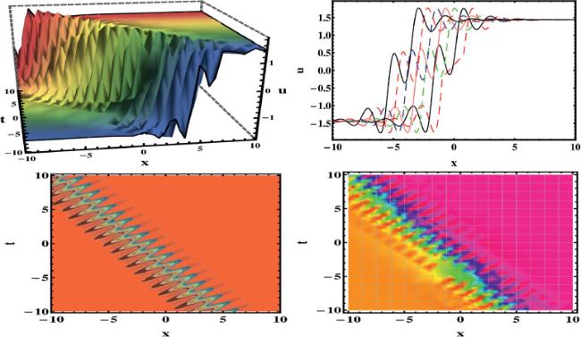
View original graphic|Download|PPT slide

Fig. 1. Plots of solution (8) with parameters $δ_{0} = 0.7, m_{1} = 2.03, ρ_{0} = 2.8, ρ_{1} = 0.72, σ_{0} = - 1.5, y = 0.01$ .

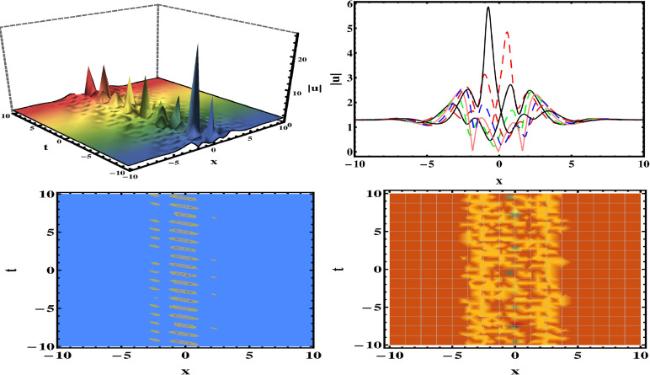
View original graphic|Download|PPT slide

Fig. 2. Plots of solution (12) with parameters $δ_{0} = 1.79, m_{2} = 1.1, m_{1} = 2, ρ_{0} = 1.4, ρ_{1} = 0.65, σ_{0} = 2.01, y = 0.09$ .

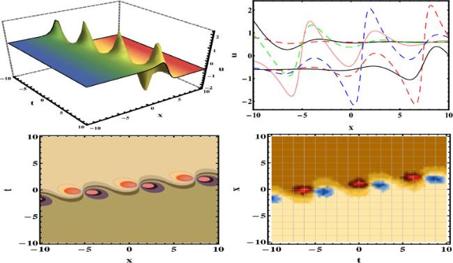
View original graphic|Download|PPT slide

Fig. 3. Plots of solution (21) with parameters $α_{2} = 0.08, b_{1} = 0.3, b_{2} = 1, γ_{5} = 1.76, q_{2} = 0.6, q_{1} = 0.8, y = 0.99, b_{4} = 0.9, b_{5} = 1.72$ .

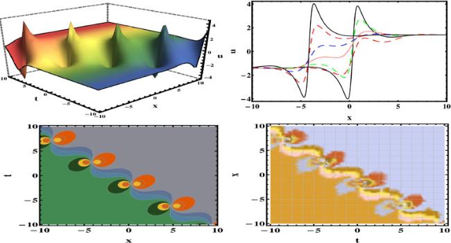
View original graphic|Download|PPT slide

Fig. 4. Plots of solution (25) with parameters $α_{2} = 0.976, b_{1} = 0.7, b_{2} = 1.1, b_{4} = 0.76, q_{2} = 0.9, q_{1} = 1, y = 0.9, b_{3} = 0.7, b_{5} = 1.98$ .

View original graphic|Download|PPT slide

Fig. 5. Plots of solution (30) with parameters $y = 1.8, a_{1} = 1.008, α_{2} = - 0.89, k = 0.9, k_{3} = 0.89, a_{3} = 1.04, a_{6} = - 0.4, k_{2} = 1.3, γ_{3} = 1$ .

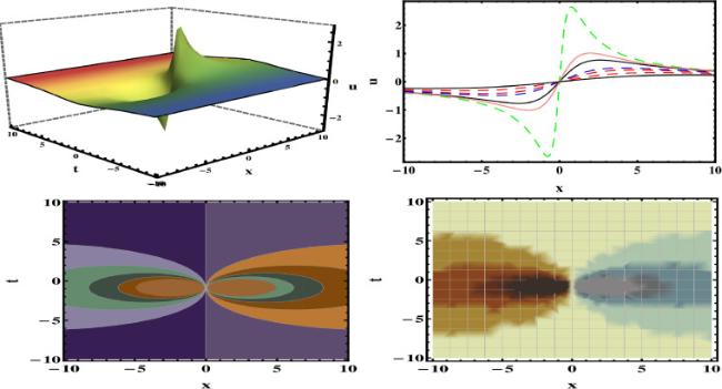
View original graphic|Download|PPT slide

Fig. 6. Plots of solution (34) with parameters $a_{1} = 2.008, a_{2} = 0.67, α_{2} = 0.7, k = 1.807, k_{3} = 0.78, y = 1.8, a_{3} = 1.09, a_{5} = 2.09, k_{2} = 0.073, γ_{4} = 1.09$ .

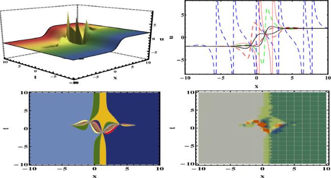
View original graphic|Download|PPT slide

Fig. 7. Plots of solution (39) with parameters $δ_{4} = 0.4, δ_{2} = 1, δ_{3} = - 2, y = 0.01, ϕ_{1} = 0.8$ .

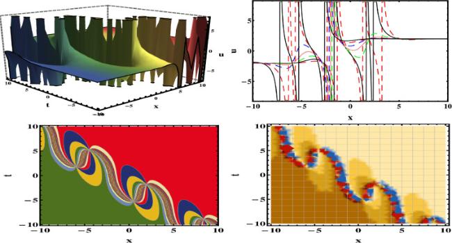
View original graphic|Download|PPT slide

Fig. 8. Plots of solution (43) with parameters $δ_{4} = 2, y = 2, ϕ_{3} = 0.91, ϕ_{2} = 0.02$ .

4. Concluding remarks

We have discussed the new exact wave structures to the generalized Hietarinta- type equation dynamic wave equation. The solutions including breather-type, lump-periodic, rouge waves and two waves solutions have been recovered by applying HBM and test function techniques. Relying on the achieved findings, experts may also apply them to physics or mathematics. Finally, with the help of Mathematica, we have put our solutions back into the governing equation and verify them. In addition, the best parameter shortlisting charts the 3D, 2D, density, and contour characteristics to deduce the physical phenomena associated with real-world secured solutions. Our established results show that the derived algorithm is an effective and reliable tool for obtaining bilinear forms of nonlinear PDEs from nonlinear dynamics, mathematics, fluid dynamics, oceanography, soliton theory, and other nonlinear sciences. Achieving such outcomes is highly recommended in cutting-edge research and development.

Declaration of Competing Interest

The authors declare that they have no known competing financial interests or personal relationships that could have appeared to influence the work reported in this paper.

Acknowledgments

The authors would like to acknowledge the financial support provided for this research via Open Fund of State Key Laboratory of Power Grid Environmental Protection (No. GYW51202101374).

References

Publishing order | Descend order by publishing year | Descend order by cited within

[1]	M.M.A. Khater, S.A. Salama. J. Ocean Eng. Sci., 7 (2022), pp. 264-271

[2]	H. F. Ismael, I. Okumuş, T. Aktürk, H. Bulut, M. S. Osman, J. Ocean Eng. Sci. 10.1016/j.joes.2022.03.017.

[3]	U. Younas, J. Ren, M.Z. Baber, M.W. Yasin, T. Shahzad, J. Ocean Eng. Sci. 10.1016/j.joes.2022.05.005.

[4]	M.M.A. Khater, S.K. Elagan, M.A. El-Shorbagy, S.H. Alfalqi, J.F. Alzaidi, N.A. Alshehri. Commun. Theor. Phys., 73 (2021), p. 095003 DOI: 10.1088/1572-9494/ac049f

[5]	M.M.A. Khater, D. Lu. Mod. Phys. Lett. B, 35 (2021), p. 2150324 DOI: 10.1142/s0217984921503243

[6]	M.M.A. Khater. Mod. Phys. Lett. B, 35 (2021), p. 2150220 DOI: 10.1142/s0217984921502201

[7]	B. Ghanbari, M.S. Osman, D. Baleanu. Mod. Phys. Lett. A, 34 (2019), p. 1950155 DOI: 10.1142/s0217732319501554

[8]	H. Rezazadeh, M.S. Osman, M. Eslami, M. Ekici, A. Sonmezoglu, M. Asma, W.A.M. Othman, B.R. Wong, M. Mirzazadeh, Q. Zhou, A. Biswas, M. Belic. Optik, 164 (2018), pp. 84-92

[9]	U. Younas, J. Ren. Results Phys., 21 (2021), p. 103816

[10]	M.S. Osman, B. Ghanbari. Optik, 175 (2018), pp. 328-333

[11]	K.K. Ali, A.M. Wazwaz, M.S. Osman. Optik, 208 (2020), p. 164132

[12]	M.S. Aktar, M.A. Akbar. Chaos Solitons Fractals, 160 (2022), p. 112212

[13]	M.M.A. Khater. Mod. Phys. Lett. B, 35 (2021), p. 2150372 DOI: 10.1142/s0217984921503723

[14]	M.M.A. Khater. Mod. Phys. Lett. B, 35 (2021), p. 2150456 DOI: 10.1142/s021798492150456x

[15]	M.M.A. Khater. Mod. Phys. Lett. B, 35 (2021), p. 2150480

[16]	U. Younas, T.A. Sulaiman, J. Ren, A. Yusuf. J. Geom. Phys., 178 (2022), p. 104586

[17]	B. Inan, M.S. Osman, T. Ak, D. Baleanu. Math. Methods Appl. Sci., 43 (2020), pp. 2588-2600 DOI: 10.1002/mma.6067

[18]	M. Adel, D. Baleanu, U. Sadiya, M.A. Arefin, M.H. Uddin, M.A. Elamin, M.S. Osman. Results Phy., 38 (2022), p. 105661

[19]	H. Rezazadeh, M. Odabasi, K.U. Tariq, R. Abazari, H.M. Baskonus. Chin. J. Phys., 72 (2021), pp. 403-414

[20]	S. Kumar, S.K. Dhiman, D. Baleanu, M.S. Osman, A.M. Wazwaz. Symmetry, 14 (2022), p. 597

[21]	M.M.A. Khater, K.S. Nisar, M.S. Mohamed. Math. Math. Method App. Sci., 44 (2021), pp. 4598-4606 DOI: 10.1002/mma.7052

[22]	M.M.A. Khater, A.A. Mousa, M.A. El-Shorbagy, R.A.M. Attia. Results Phys., 22 (2021), p. 103954

[23]	M.M.A. Khater, M.S. Mohamed, R.A.M. Attia. Chaos Solitons Fractals, 144 (2021), p. 110676

[24]	M.M.A. Khater, A.E.S. Ahmed, M.A. El-Shorbagy. Results Phys., 22 (2021), p. 103890

[25]	U. Younas, J. Ren. J. Ocean Eng. Sci. (2022), DOI: 10.1016/j.joes.2022.04.014.

[26]	U. Younas, M. Bilal, J. Ren. J. Magn. Magn. Mater., 549 (2020), p. 168995

[27]	K.K. Ali, R. Yilmazer, M.S. Osman. Opt. uant. Electron., 54 (2022), p. 160

[28]	S. Tarla, K.K. Ali, R. Yilmazer, M.S. Osman. Opt Quant Electron, 54 (2022), p. 292

[29]	S. Kumar, R.P. Chauhan, M.S. Osman, S.A. Mohiuddine. Math. Method App. Sci. (2021), DOI: 10.1002/mma.7838.

[30]	U. Younas, M. Bilal, T.A. Sulaiman, J. Ren, A. Yusuf. Opt. Quant. Electron., 54 (2022), p. 71

[31]	M.M.A. Khater, B. Ghanbari. Eur. Phys. J. Plus, 136 (2021), p. 447

[32]	M.M.A. Khater, T.A. Nofal, H. Abu-Zinadah, M.S.M. Lotayif, D. Lu. Alex. Eng. J., 60 (2021), pp. 1797-1806

[33]	M.M.A. Khater, M.S. Mohamed, S.K. Elagan. Results Phys., 23 (2021), p. 104003

[34]	M.M.A. Khater, M.S. Mohamed, S.K. Elagan. Results Phys., 23 (2021), p. 104003

[35]	M.M.A. Khater, S. Anwar, K.U. Tariq, M.S. Mohamed. AIP Adv., 11 (2021), p. 025130

[36]	S.J. Chen, X. Lu, W.X. Ma. Commun. Nonlinear Sci. Numer. Simul., 83 (2020), p. 105135

[37]	U. Younas, J. Ren, T.A. Sulaiman, M. Bilal, A. Yusuf. Mod. Phys. Lett. B (2022), DOI:

[38]	S.T.R. Rizvi, A.R. Seadawy, F. Ashraf, M. Younis, H. Iqbal, D. Baleanu. Eur. Phys. J. Plus, 134 (3) (2019), pp. 1-10 DOI: 10.11114/bms.v5i2.4062

[39]	I. Ahmed, A.R. Seadawy, D. Lu. Int. J. Mod. Phys. B, 33 (2019), p. 1950019

[40]	L. Kaur, A.M. Wazwaz. Phys. Scr., 93 (7) (2018), p. 075203 DOI: 10.1088/1402-4896/aac8b8

[41]	A. Yusuf, T.A. Sulaiman, M. Inc, M. Bayram1. Eur. Phys. J. Plus, 135 (7) (2020), pp. 1-8

[42]	M. Younis, S.T.R. Rizvi, D. Baleanu, H. Iqbal. Chin. J. Phys., 68 (2020), pp. 19-27 DOI: 10.32323/ujma.622495

[43]	C.H. He, Y. Tang, W.X. Ma, J. Ma. Nonlinear Dyn., 95 (2019), pp. 29-42 DOI: 10.1007/s11071-018-4548-8

[44]	M. Singh. Nonlinear Dyn., 84 (2016), pp. 875-880 DOI: 10.1007/s11071-015-2533-z

[45]	J. Manafian, O.A. Ilhan, A. Alizadeh. Math. Methods Appl. Sci. (2020), pp. 1-24

[46]	Y.L. Ma, B.Q. Li. Comput. Math. with Appl., 78 (2019), pp. 827-839

[47]	V.E. Zakharov. Dokl. Akad. Nauk SSSR, 228 (1976), pp. 1314-1316

[48]	A.D.D. Craik, J.A. Adam. Proc. R. Soc. A, 363 (1978), pp. 243-255

[49]	C. Kharif, E. Pelinovsky. Eur. J. Mech. B Fluids, 22 (2003), pp. 603-634

[50]	S. Batwa, W.X. Ma. Front. Math. China, 15 (2020), pp. 435-450 DOI: 10.1007/s11464-020-0844-y

[51]	Y. Feng, S. Bilige. Pramana - J. Phys., 95 (2022), p. 151 DOI: 10.18653/v1/2022.findings-naacl.12

[52]	M.R.A. Fahima, P.R. Kundua, M.E. Islama, M.A. Akbar, M. S. Osman. J. Ocean Eng. Sci., 7 (2022), pp. 272-279

[53]	I. Jaradat, M. Alquran. J. Ocean Eng. Sci., 7 (2022), pp. 244-247

[54]	M.A. Arefin, M.A. Khatun, M.H. Uddin, M. Inc. J. Ocean Eng. Sci., 7 (2022), pp. 292-303

Options

Outlines

模态框（Modal）标题

Abstract

Cite this article

1. Introduction

2. Interaction aspects

2.1. Breather-type waves

2.2. Lump-periodic solutions

2.3. Rogue wave solutions

2.4. Two-wave solutions

3. Discussion

Fig. 1. Plots of solution (8) with parameters δ 0 = 0.7 , m 1 = 2.03 , ρ 0 = 2.8 , ρ 1 = 0.72 , σ 0 = − 1.5 , y = 0.01.

Fig. 2. Plots of solution (12) with parameters δ 0 = 1.79 , m 2 = 1.1 , m 1 = 2 , ρ 0 = 1.4 , ρ 1 = 0.65 , σ 0 = 2.01 , y = 0.09.

Fig. 3. Plots of solution (21) with parameters α 2 = 0.08 , b 1 = 0.3 , b 2 = 1 , γ 5 = 1.76 , q 2 = 0.6 , q 1 = 0.8 , y = 0.99 , b 4 = 0.9 , b 5 = 1.72.

Fig. 4. Plots of solution (25) with parameters α 2 = 0.976 , b 1 = 0.7 , b 2 = 1.1 , b 4 = 0.76 , q 2 = 0.9 , q 1 = 1 , y = 0.9 , b 3 = 0.7 , b 5 = 1.98.

Fig. 5. Plots of solution (30) with parameters y = 1.8 , a 1 = 1.008 , α 2 = − 0.89 , k = 0.9 , k 3 = 0.89 , a 3 = 1.04 , a 6 = − 0.4 , k 2 = 1.3 , γ 3 = 1.

Fig. 6. Plots of solution (34) with parameters a 1 = 2.008 , a 2 = 0.67 , α 2 = 0.7 , k = 1.807 , k 3 = 0.78 , y = 1.8 , a 3 = 1.09 , a 5 = 2.09 , k 2 = 0.073 , γ 4 = 1.09.

Fig. 7. Plots of solution (39) with parameters δ 4 = 0.4 , δ 2 = 1 , δ 3 = − 2 , y = 0.01 , ϕ 1 = 0.8.

Fig. 8. Plots of solution (43) with parameters δ 4 = 2 , y = 2 , ϕ 3 = 0.91 , ϕ 2 = 0.02.

4. Concluding remarks

Declaration of Competing Interest

Acknowledgments

References

Links

Fig. 1. Plots of solution (8) with parameters $δ_{0} = 0.7, m_{1} = 2.03, ρ_{0} = 2.8, ρ_{1} = 0.72, σ_{0} = - 1.5, y = 0.01$ .

Fig. 2. Plots of solution (12) with parameters $δ_{0} = 1.79, m_{2} = 1.1, m_{1} = 2, ρ_{0} = 1.4, ρ_{1} = 0.65, σ_{0} = 2.01, y = 0.09$ .

Fig. 3. Plots of solution (21) with parameters $α_{2} = 0.08, b_{1} = 0.3, b_{2} = 1, γ_{5} = 1.76, q_{2} = 0.6, q_{1} = 0.8, y = 0.99, b_{4} = 0.9, b_{5} = 1.72$ .

Fig. 4. Plots of solution (25) with parameters $α_{2} = 0.976, b_{1} = 0.7, b_{2} = 1.1, b_{4} = 0.76, q_{2} = 0.9, q_{1} = 1, y = 0.9, b_{3} = 0.7, b_{5} = 1.98$ .

Fig. 5. Plots of solution (30) with parameters $y = 1.8, a_{1} = 1.008, α_{2} = - 0.89, k = 0.9, k_{3} = 0.89, a_{3} = 1.04, a_{6} = - 0.4, k_{2} = 1.3, γ_{3} = 1$ .

Fig. 6. Plots of solution (34) with parameters $a_{1} = 2.008, a_{2} = 0.67, α_{2} = 0.7, k = 1.807, k_{3} = 0.78, y = 1.8, a_{3} = 1.09, a_{5} = 2.09, k_{2} = 0.073, γ_{4} = 1.09$ .

Fig. 7. Plots of solution (39) with parameters $δ_{4} = 0.4, δ_{2} = 1, δ_{3} = - 2, y = 0.01, ϕ_{1} = 0.8$ .

Fig. 8. Plots of solution (43) with parameters $δ_{4} = 2, y = 2, ϕ_{3} = 0.91, ϕ_{2} = 0.02$ .