
1. Introduction
In [1], the first 3D autonomous chaotic system was found by Lorenz when he investigated atmospheric convection. Lorenz system has been taken as a first model for studying chaos. After that, in [2], Rӧssler built a simpler chaotic 3D system. It is noteworthy that during the past twenty years, the chaos of technological paradigms, like nonlinear electric circuits, has progressively shifted from a pure science to a promising subject that has important applications. It is observed that intentionally generating chaos is a vital case in several technical implementations. In this direction, Chen built a three-dimensional autonomous chaos model [3,4] based on an engineering approach to feedback control, after that Lü has built his system [5] and general model combining all cases as a special case has built and named the unified model [6]. Following Vanecek and Celikovsky's classification of canonical form [7], in the 3D autonomous paradigms that have quadratic nonlinearities, considering the linear term ( ), the Lorenz model fulfils , the Chen model fulfils , and the Lü model fulfils although they aren't topologically equivalent. With this direction, they form together a full collection of general Lorenz dynamical models. From another point of view, the Rӧssler system contains a quadratic cross product term and is not part of the general family of Lorenz systems mentioned above. Recently, during the study of a 3D Rӧssler-type autonomous chaotic model with quadratic cross product terms, Liu and Chen [8] constructed a chaotic model with a quadratic product term in every kernel, that could give two attractors at the same time each of which has a double-scroll.
The concept of fractional calculus has been recognized since the evolution of the ordinary one, and its origin probably relates to a 1695 communication of Leibniz and L' Hospital. They discussed the concept of 1.5 order derivative [9]. Despite the long age of the fractional derivation, its applications in physics and engineering are still recent. Much research has been devoted to the creation of chaos using autonomous fractional order nonlinear models. In [10], fractional order chaos and hyper chaos were examined for the Rӧssler model. In [11], system synchronization of fractional order was performed. Control and stability for a collection of fractional-order nonlinear models have been investigated with Caputo derivative in [12]. The fractional order derivative provides many features to the dynamical system. It takes the history of the system dynamics into account. And the order of the derivative increases the number of parameters of the chaotic model. So, we can get new chaotic attractors and increases the dimension of parameters' space which increase its efficiency in secure communication applications. Also, in modelling, the fractional order can be used as a tuner parameter for the response to meet the modelled phenomena. But the classical derivatives and the models based on them do not consider any memories and hereditary effects. Extra fractional and integer order chaotic models and applications can be found in [13], [14], [15], [16], [17], [18], [19], [20] and [30], [31], [32], [33], [39], [40], [41].
Dynamical systems, especially the chaotic ones are widely utilized to model Ocean and atmospheric dynamics. Ocean engineering is interested with large scale wave motions in the Ocean (for example, wind waves, tsunami waves) and air along with the temperature and density of water in the Ocean. Ocean and atmosphere are equally significant in transferring energy between positions in the form of wave propagation. Dynamical systems, especially the chaotic ones help to model various phenomena in Oceans. Several research works have highlighted the values of eddies and chaos inside the Ocean in controlling the response to forcing from climate change. Certain physical processes in the Ocean produce highly non-linear or chaotic fluctuations. In [34], Jianmin Yang and Wenyue Lu numerically studied the generation and evolution of the super-rogue waves. In [35], the reader can see the importance of dynamical systems in modelling and evaluation of dynamics of jack-up platform system under wave, wind, earthquake, and tsunami loads. More numerical and computational studies of dynamical systems can be found in [36], [37], [38].
Encouraged by the previous studies, a new fractional chaotic 6D model is constructed which can be used to model may Oceanic phenomena. We proved the chaos nature of the proposed new fractional 6D model numerically by displaying its dynamics related to the order of the fractional differentiation. The Lyapunov exponents and bifurcation maps of the proposed model is presented. The impact of the order of the fractional differentiation on the Lyapunov exponent are presented. The structural properties of the proposed 6D model are studied via certain graph theory tools. In addition, the proposed 6D 5.4-fractional order chaotic model is realized by constructing an electronic circuit and we present its response. Also, an active fractional controller is produced to control the presented 6D fractional chaotic model.
The remaining of the manuscript is arranged as: the preliminaries and basic definitions of fractional differentiation are given in Section 2. The 6D chaotic model is constructed and its basic characteristics are given in Section 3. The new attractors are displayed in Section 4. Certain structural features of the proposed 6D chaotic model are presented using graph theory tools in Section 5. Section 6 contains the electronic circuit realization of the proposed fractional 6D chaotic model. An active fractional controller is designed and applied for the studied chaotic model in Section 7. The conclusions of our study are put in Section 8.
2. Fractional derivative and its preliminaries and basic definitions
This section briefly describes the fractional derivative and its corresponding fractional integral. Several notations were used in the new definition of fractional derivative. Through this article, we use and respectively for the fractional differentiation and its corresponding integration, where signifies the integration lower limit and is the order of the fractional derivative or fractional integral. For each , and for any function , and should meet the following criteria [21]:
If is analytic function, then the operator and are analytic w.r.t. .
The fractional differentiation operators satisfy the following linearity rules:
The fractional operators with zero order must have no effect on , i.e.,
If is a positive integer, the fractional operator should give the same result as a normal derivative or integral.
In the coming parts, the Caputo fractional operators of differentiation and integration are introduced in its common sense which defined as following [22] and shall be used to construct the proposed new chaotic model.
For more details and other definitions as Atangana-Baleanu derivative and Caputo-Fabrizio derivative with its possible applications can be found in [23].
Definition 1. The following formula represents the Laplace transformation of Caputo fractional order operator
Definition 2. For the graph , define the matrix , such that if is adjacent to in and otherwise. A is called adjacency matrix of
Definition 3. The Hermitian matrix of a digraph is defined as:
The basics of the graph theory and its applications can be found for example in [24]
3. The novel 6D chaotic model and its basic characteristics
In the following, let us write as . The 6D nonlinear fractional autonomous novel system is described by
where ( ) are the state variables of the proposed model, and are the model parameters and all of them are positive real constants.
Constructing this model and determining the values of its parameters such that the model has chaotic dynamic follow some common concepts of chaotification [25,26], to build an autonomous chaotic paradigm or to chaotic a non-chaotic autonomous paradigm, the coming framework rules need to be satisfied:
i) Dissipative of the model, in other words, the energy of the model is diminishing (except if Hamiltonian models are taken into consideration).
ii) The model has an unstable equilibrium. In other words, the equilibrium-evaluated Jacobian value has unstable eigenvalues.
iii) The model consists of one cross product term at least. That is, the dynamic effects between different variables can be considered.
iv) All system trajectories are bounded. In other words, dynamic equilibrium is maintained by increasing and decreasing system energy.
The method of chaotifying the discrete models have some systematic steps [25], but there are no general techniques for non-discrete cases. In the latter case, the above analytical conditions usually need to be combined with trial-and-error computer experiments to accomplish the needed chaotic job. System (6) is also has such a shape. Now, some basic features of (6) are examined.
In the following subsections, some basic characteristics of the proposed system (6) are examined.
3.1. Dissipative feature for the proposed model (6)
The 6D nonlinear fractional autonomous novel system is described by
For this model (7), let , we have
Then, system (7) is dissipative, if
Suppose that is a suitable region in which has a smooth boundary and let such that is the flow of the vector field . Plus, let that the volume of is . Referring to Liouville's theorem as in [13], we get
Then from (7) and (9), we have
Integrating (11), then
from (12), we conclude that the orbit of this dynamic model (6) forces all contained volumes to be reduced to zero. Therefore, there are attractors that attract all the orbits of the new model. From this, we can show that the newly proposed chaos model (6) is dissipative in the following condition is met:
3.2. Model (6) equilibrium points
The equilibrium points of the proposed model (6) can be found by simultaneously solving the next equations:
Clearly, is one of the equilibrium points. The system is very complex and has many other equilibrium points that can be calculated using Matlab. Here, the stability of the zero equilibrium is examined only. The Jaccobian can be obtained by linearizing system (6) at as:
That has the following eigenvalues:
, ,
Since all model parameters are positive real numbers, it is easy to find that , proving the instability of the equilibrium . The other nonzero equilibria, it is still possible to numerically evaluate their stabilities. Since two unstable equilibriums has been got at , this long numerical calculation becomes not needed then it is not examined further here.
4. Displaying of new chaotic attractors
In the following, to simplifying the study, the produced model parameters are taken as: , , and . Then proposed model is rewritten as follows.
Considering condition (12), with initial conditions and fractional order , many numerical experiments have been executed, certain discoveries recorded as follows.
4.1. Varying the fractional order with
Fig. 1 displays the spectrum of Lyapunov exponents versus the order of fractional derivative and parameters are chosen as From which one can note that LE1 and LE2 are positive for fractional order . In Table 1, some values of Lyapunov exponents are recoded against different values of . The proposed system (18) has a hyperchaotic behavior for the fractional order . Fig. 2 shows the bifurcation map of related to the fractional order where parameters are chosen as Fig. 3, Fig. 4, show two hyperchaotic attractors at fractional orders 0.9 and 1 respectively. For outside this period , the system has fixed point behavior as shown in Fig. 5.
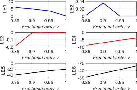
Fig.1 Lyapunov exponents spectrum versus the fractional order where the model parameters are fixed as |
Table 1 Lyapunov exponents of the proposed system (18) for various values of fractional order v. |
| Fractional order v | LE1 | LE2 | LE3 | LE4 | LE5 | LE6 |
|---|---|---|---|---|---|---|
| 0.8515 | 5.9389 | 0.0031 | -0.1850 | -8.7262 | -40.1658 | -57.4287 |
| 0.9010 | 4.9808 | 0.0362 | -0.0060 | -6.9942 | -32.1153 | -46.8727 |
| 0.9505 | 3.6936 | 0.0006 | -0.0006 | -5.3108 | -25.4198 | -37.3238 |
| 1 | 0.3514 | 0.0007 | -0.0068 | -3.8473 | -19.9668 | -27.2099 |
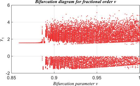
Fig.2 Bifurcation map of related to the fractional order where the model parameters are fixed as |

Fig.3 Hyperchaotic attractor of the proposed model (18) at fractional order and |
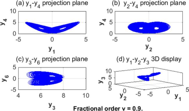
Fig.4 Hyperchaotic attractor of the proposed model (18) at fractional order and |
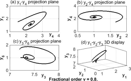
Fig.5 Fixed point behavior of the proposed model (18) at fractional order and |
From above experiments, the proposed system is hyperchaotic for fractional order where model parameters are selected as
4.2. Vary the parameter a and fix
As clear from Fig. 6, the spectrum of Lyapunov-exponents show that the proposed model (18) is hyperchaotic for a wide range of the parameter for fractional order and the system lose its chaotic dynamical behavior outside this period. Fig. 7 displays the bifurcation maps of related to parameter where other parameters are selected as at different fractional orders.
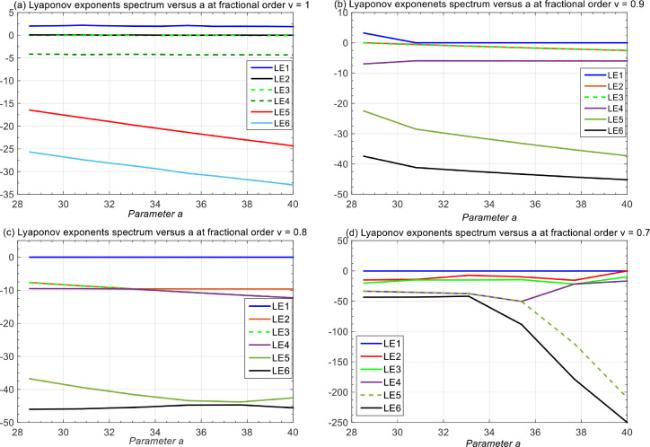
Fig.6 Lyapunov exponents spectrum versus the parameter where other parameters are fixed as at different fractional orders . |
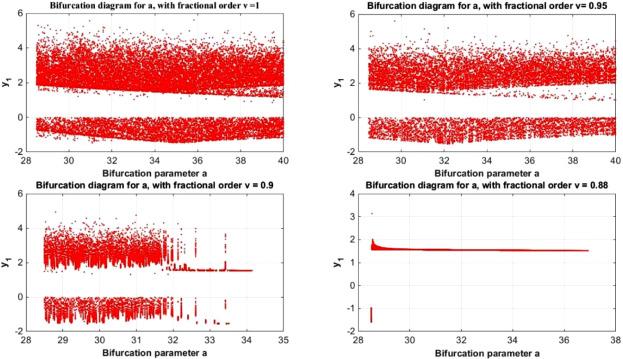
Fig.7 Bifurcation maps of related to parameter where other parameters are selected as at different fractional orders . |
5. Structural characteristic of proposed model (18)
In this section, we display the relations between the different terms of the proposed model via drawing its graph. The proposed model consists of pure state variables and nonlinear product terms. We draw the suggested graph as follows. The graph vertices are the six pure state variables plus the eight nonlinear product terms. There will be a directed edge between two vertices if the corresponding terms affect the other. For example, there will be a directed edge from the vertex corresponds to the term to the vertex corresponds to the term , but there no edge from the vertex corresponds to towards that corresponds to , so model (18) can be displayed by the digraph given in Fig. 8. Many structural characteristics of the model can be calculated from the adjacency and Hermitian matrices.
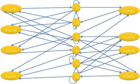
Fig.8 The digraph of the studied chaotic model. |
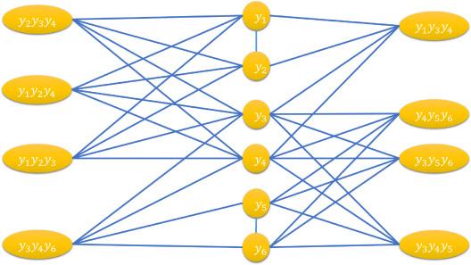
The underlying graph (shown in Fig. 9) of a digraph is constructed by neglecting the direction of the edges and the loops (edges with same ends). Following Definitions 2, 3, respectively, the adjacency matrix for the underlying graph of and the Hermitian matrix for the model digraph are constructed as follows in (19) and (20).
The eigenvalues of are:
. And the eigenvalues of H(D) are: .
The energy of the graph is defined as , where 14 is the order of and 's are the eigenvalues of its adjacency matrix. This idea was presented by I. Gutman in [24] and has several applications and it can be utilized to estimate the whole energy of graphs. The Hermitian energy is defined as where 14 is the order of and 's are the eigenvalues of its Hermitian matrix.
6. Electric circuit realization of the studied fractional chaotic system
In this section, we show that the proposed chaotic model is applicable by constructing its electric circuit. By constructing an electric circuit for the proposed model, we prove its ability to be applicable in real world applications. Here, we consider the suggested 6D fractional order chaotic paradigm (18). First, we fix the fractional order to design circuit to realize model (18). We follow the method published in [27] to realize . With aid of NI Multisim 14.0 package, the electric circuit given in Fig. 10 is designed, where S1, S2, ..., S6 are six summers all of them has 3 inputs and single output; M1, M2, …, M11 are AD633 voltage multiplier with 2 inputs and single output all of them are adjusted with identity gain; six LM741 op. amp's are utilized to simulate the six 0.9-fractional-order voltage integrators with outputs equal the states of the system to ; R1, R2, R3, R4, R5, R15 are 100K resistances and R6, R7, R8, R9 are 10KΩ resistances plus a couple of LM741 op. amps. are used to construct two voltage inverters. The designed values of resistors and capacitors are given in Tables 2 and 3. In Table 4, we record input/output gain's utilized in voltage summers. The electronic circuit implementing the new chaotic 6D model (18) is shown in Fig. 10. Figs. 11 and 12 display the response of 5.4-fractional-order chaotic 6D new model.
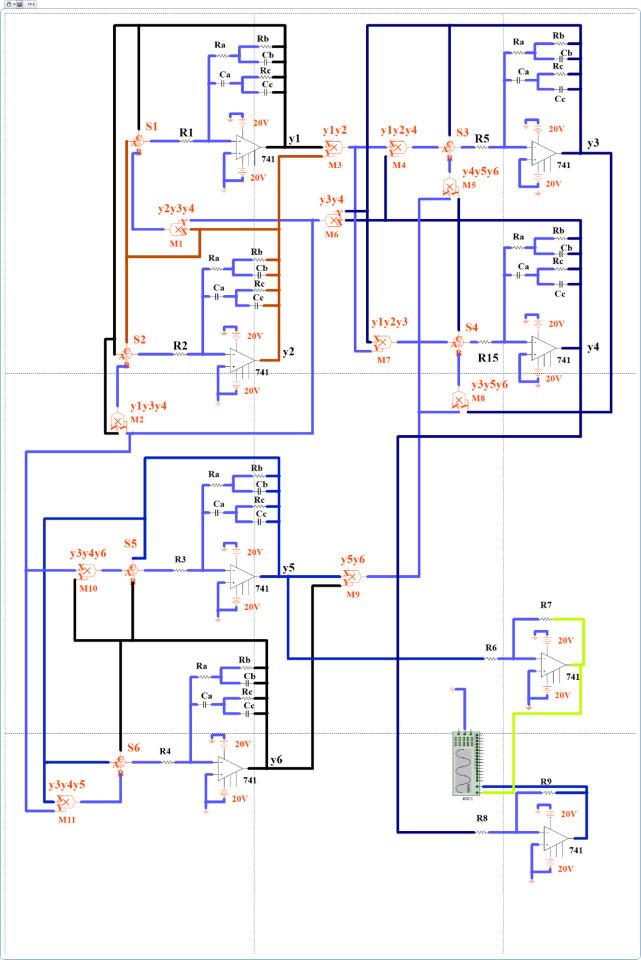
Fig.10 Electronic circuit implementing the 5.4-fractional-order 6D new chaotic model (18). |
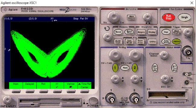
Fig.11 - phase plane from the electronic circuit of the 5.4-fractional-order 6D new chaotic model (18). |
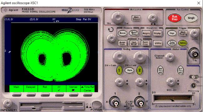
Fig.12 - phase plane from the electronic circuit of the 5.4-fractional-order 6D new chaotic model (18). |
Table 2 The tree shape (2dB) integrator: values of resistors (c.f. [27]). |
| 0.9 |
Table 3 The tree shape (2dB) integrator: values of capacitors (c.f. [27]). |
| 0.9 |
Table 4 The used voltage summing devices': gains for inputs (A, B, C) and output O. |
| summer symbol | A | B | C | O |
|---|---|---|---|---|
| S1 | -30 | -1 | 30 | 0.28 |
| S2 | -10 | 1 | 10 | 0.28 |
| S3 | -1 | -1 | 1 | 0.015 |
| S4 | -1 | -1 | 10 | 0.015 |
| S5 | -1 | -30 | 30 | 0.28 |
| S6 | -10 | 1 | -10 | 0.28 |
7. Design of fractional order active controller for the proposed chaotic model (18)
In this section, we propose an active control strategy to control the model states and convert it to a fixed point.
For the proposed system (18), the control rule is designed as follows:
where 's are control gains. The controlled model becomes:
Substituting (21) into (22), the dynamics of the controlled model becomes:
It is obvious that the controlled system (23) has as an equilibrium point. The following theorem can be proved for the controlled fractional order model (23).
Theorem 1. If all controller gains 's in the controlled model (23) are chosen to be negative values, then of the controlled model (23) is fixed point.
Proof. Taking Laplace transformation for the controlled model (23), then
then
where is the Laplace transformation of so
applying inverse taransformation of Laplace for (24), we get
such that is the common function of Mittag-Leffler. Because , so approaches zero for all values of if all 's are negatives, the reader can consult [28], [29] and its cited references for more about function of Mittag-Leffler. Then, the states of the model are all stable asymptotically. Figs. 13, 14 and 15 show the time response of the new fractional 6D chaotic model before and after control at fractional order respectivily with all gains . The controller is applied after 30 secs. We can see that the model takes a transient time to reach its final state. Changing the controller gains to be , the transient time is approaches zero as shown in Figs. 16, 17 and 18.
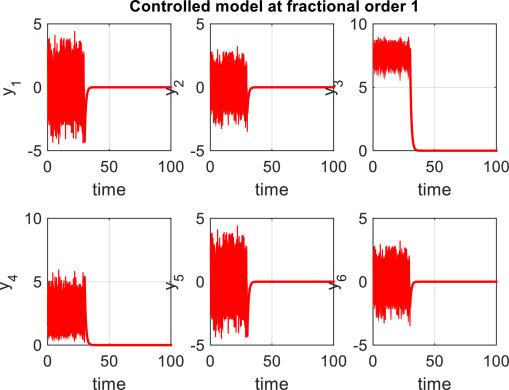
Fig.13 Dynamics of the new fractional 6D chaotic model before and after control at fractional order , with all gains . |
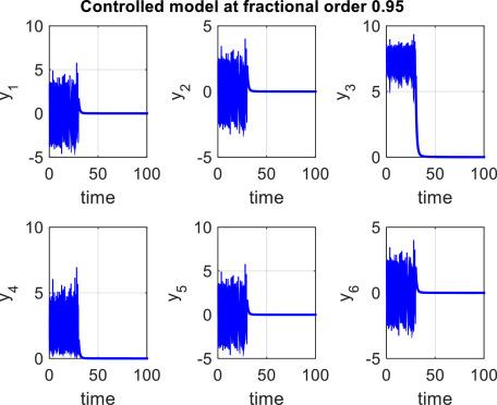
Fig.14 Dynamics of the newfractional 6D chaotic model before and after control at fractional order , with all gains . |
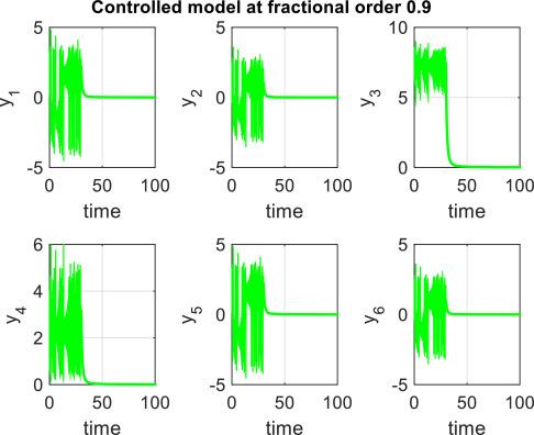
Fig.15 Dynamics of the newfractional 6D chaotic model before and after control at fractional order , with all gains . |
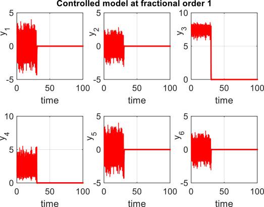
Fig.16 Dynamics of the newfractional 6D chaotic model before and after control at fractional order , with all gains . |
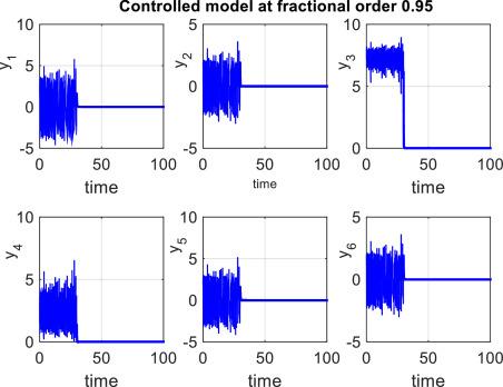
Fig.17 Dynamics of the newfractional 6D chaotic model before and after control at fractional order , with all gains . |
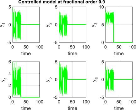
Fig.18 Dynamics of the newfractional 6D chaotic model before and after control at fractional order , with all gains . |
8. Conclusions
The new fractional 6D chaotic model presented above has complicated behaviors and all characteristics of the chaotic system. The proposed fractional 6D chaotic system with different topology and structure than the existing 6D systems is constructed in this work. The basic features and dynamical response of the new model have been investigated to prove it's chaotic. Certain graph theory tools have been utilized to display some hidden properties of the proposed model. In addition, an electronic circuit realizing the proposed model has been designed. Also, an active fractional controller is proposed to control the proposed model. In the future work, we suggest utilizing this fractional 6D model to produce random keys for data encryption and in secure communication applications.
Data Availability Statement
Not applicable.
Author contributions
Conceptualization, M.H.; methodology, M.H., N.A.; software, M.H., S.M., A.A., N.A.; validation, M.H., S.M., A.A., N.A; formal analysis, M.H., S.M., A.A., N.A.; investigation, M.H., S.M., A.A., N.A; resources, M.H., S.M., A.A., N.A.; data curation: M.H.; Funding acquisition, M.H., S.M., A.A., N.A.; writing—original draft preparation, M.H.; writing—review and editing, M.H., S.M., A.A., N.A; visualization, M.H.; supervision, M.H.; project administration, M.H., S.M., All authors have read and agreed to the published version of the manuscript.
Funding
The authors acknowledge the support and funding of Research Center for Advanced Material Science (RCAMS) at King Khalid University through Grant No. RCAMS/KKU/009-21.
Declaration of Competing Interest
The authors declare no conflict of interests.
Acknowledgements
The authors acknowledge the support and funding of Research Center for Advanced Material Science (RCAMS) at King Khalid University through Grant No. RCAMS/KKU/009-21.
