
1. Introduction
1.1. Scope
In the physical sciences, nonlinear partial differential equations (NPDEs) are frequently employed to describe complicated processes. Thus, the problems/models arising in ocean science [1], [2], [3], [4], [5], [6], [7], [8], [9], [10], [11], [12], [13], [14], [15], [16], [17], [18], [19], [20], [21], [22], [23], oceanography [24], mathematical physics [25], complex fluid flows [26], [27], plasma physics [28], electromagnetic theory, fluid dynamics [29], [30], nuclear physics, chemical physics, to name a few [31], [32], [33], [34], [35], [36], [37], [38], [39], [40], [41], [42], [43], [44], [45], [46], [47], [48], [49], [50], [51], [52], [53], [54], [55], [56], [57], [58], [59], [60], [61], [62], [63], [64], [65], [66], [67], [68], [69] are not easily solvable and finding their analytical solutions is critical. Reviewing the existing literature [25], [26], [27], [28], [29], [30], [31], [32], [33], [34], [35], [36], [37], [38], [39], [40], [41], [42], [43], [44], [45], [46], [47], [48], [49], [50], the authors are motivated to solve the following ( )-coupled Drinfel'd-Sokolov-Wilson equations (CDSWEs) system analytically. The system is governed by
where , , and are non-zero parameters, , are space and time variables, respectively, while and depict the components of nonlinear surface gravity waves travelling horizontally on the seabed.
Gravity waves are formed in a fluid medium or at the interface of two media when gravity or buoyancy trying to restore equilibrium. The contact between the atmosphere and the ocean, which causes wind waves, is an example of such an interaction. In deeper water, a long water wave moves faster. In deeper water, gravity waves have a faster phase speed than in shallow water. Shallow water waves (SWW) are helpful to classify the marine environment, investigate ocean dynamics, and model equatorial tsunami waves. During their propagation, SWW are influenced by the ocean floor, causing the orbital motion of water to be disrupted. As a result, they may cause underwater earthquakes, and unimaginable damage to the coastal ecology. On the other hands, the heights, wave lengths, and time durations of gravity waves frequently vary as they advance in different directions [1]. Gravity waves in shallow water are dispersion (water waves) and non-dispersive as the depth is substantially smaller than the wavelength. Nonlinear interactions between triads of wave components with frequencies and vector wave numbers satisfying following conditions which affect ocean surface gravity waves [2].
1.2. Origin of the problem
It is essential to consider the following form Hirota et al. [3] of coupled Korteweg-de Vries (KdV):
which represents the interaction of two long waves with distinct dispersion relations, in which is a non-zero parameter and and are similar as described in CDSWEs (1).
The system (3) is integrable and can be reformulated as six-reductions of the Kadomtsev-Petviashvili hierarchy. The general construction of the KdV system (3) can be deduced using affine Lie algebras [3], while Drinfel'd and Sokolov [4] established that the general construction of the KdV system (3) can be derived using affine Lie algebras (ALA). Wilson established a link between the Kac-Moody Lie algebra [5] and KdV (3). Wilson [6] used ALA to obtain a particular variant of Eq. (1) with , , , and as inputs. One of the universal models is the CDSWEs (1), which have an infinite number of conservation laws and an integrable system [3].
1.3. Literature review
The authors are inspired by the characteristics of CDSWEs (1). The research community [25], [26], [27], [28], [29], [30], [31], [32], [33], [34], [35], [36], [37], [38], [39], [40], [41], [42], [43], [44], [45], [46], [47], [48], [49], [50] solved the system (1) using different approaches and addressing different concerns. Singh et al. [25] employed a fractional time derivative and a homotopy perturbation technique to get a solitary wave solution in the Caputo sense. The travelling wave solutions were obtained by Khan et al. [26] using a modified simple equation approach. Lu et al. [27] have employed first integral technique and obtained exponential and rational functions types solutions. Homotopy analysis has been used by Arora and Kumar [28] to establish a convergent series with two initial conditions. To get a solitary wave solution, Arnous et al. [29] applied two approaches to obtain a solitary wave solution which were the Bäcklund transformation of the Riccati equation and the trial function approach. Using the F-expansion method, Akbar and Ali [30] derived hyperbolic, rational, single soliton, and periodic solutions.
For solving time-fractional DSW systems and obtaining a solution in the form of a truncated series, Chen et al. [31] compared the coupled fractional reduced differential transform method with the residual power series method. Tariq and Seadawy [32] tackled the equation using an auxiliary equation and derived traveling and solitons solutions. The Jacobi elliptic function method was employed by Yao [33] and attained kink, bell-shaped, singular, and periodic solutions. Lu et al. [34] exploited the extended auxiliary and equation mapping methods to obtain a solution in the form of a moving and solitary wave for the same system of equations with odd and even order partial derivatives. For the CDSWEs (1), Wen et al. [35] applied bifurcation and qualitative analysis of dynamical systems to obtain solitary wave, periodic, kink shaped solutions.
Javeed et al. [36] used the first integral approach to construct a nontrivial solution to a coupled space-time fractional DSW system with Riemann-Liouville and conformable types of derivatives. For the space-time fractional derivative of the classical DSW system, Shehata et al. [37] employed the Kudryashov method to obtain a travelling wave solution. In order to determine unique periodic and solitary wave solutions for CDSWEs (1), Zhang [38] employed a semi-inverse variational approach, whereas Bibi et al. [39] used the Tanh and expanded Tanh methods and generated kink and soliton solutions. Bhatter et al. [40] exploited fractional homotopy analysis and obtained bell-shaped solutions to the nonlinear CDSWEs using a fractional operator. The -expansion method was used by Matjila et al. [41], Shi et al. [42], and Khan et al. [43] who obtained different forms of the solutions like travelling waves, hyperbolic, and trigonometric, rational, bell-shaped soliton, kink, and solitary waves.
Hirota et al. [3] established a special type of solitons for CDSWEqs. (1) i.e. static solitons, if , , and . They [3] claimed that when using Painlevé to deform CDSWEs into Bilinear form, such solitons can not be deformed when interacting with other moving solitons, whereas Ali Akbar et al. [44] used the modified alternative -expansion method to extract travelling wave solutions for the same form of equations.
Using , , and in system (1), Zhao and Zhi [45] utilised the F-expansion approach to get Jacobi elliptic, rational, solitary, and periodic solutions; and Ullah et al. [46] used the optimal homotopy method to provide doubly periodic wave solutions. The Adomian decomposition method was used by Inc [47] to determine the system's Jacobi elliptic solution
A different form of CDSWEs is examined for specific values of , , , and in Eq. (1), Morris and Kara [48] established a travelling wave solution using Lie symmetry and conservation laws. Using Ibragimov's technique, Zhang and Zhao [49] created a one-dimensional optimal system. They [49] solved the additional reductions using the simple equation approach and then extracted the polynomial solutions, whereas Zhao et al. [50] applied Lie symmetry analysis and conservation laws to the identical form of DSWEs but did not solve the reductions further. This paved the way for more solutions of DSWEs.
1.4. Motivation
Making use of the similarity transformations method (STM) via one-parameter Lie symmetry analysis, the authors derived several types of novel analytical solutions. Sophus Lie created the Lie symmetry analysis as an ad-hock integration technique for the system of PDEs. The system of differential equations is still invariant after each similarity reduction. In a system of PDEs, the STM decreases the number of independent variables by one. Using the STM repeatedly can obviously reduce the system to an equivalent system of ordinary differential equations (ODEs). Due to the invariance of STM, a system of PDEs might result in a linear system of new over-determining system of PDEs that enables one to find infinitesimal generators that are functions of the independent and dependent variables. Such adjustments, which employ Lagrange's equation as a tool, result in similarity variables and similarity functions. Substituting the value of the dependent variable in terms of a similarity function can reduce the given system of PDEs to a new system. This process is repeated until one gets a system of ODEs. On solving it, it provides solutions to the system. For a description of the STM and its uses, one might look through the extensive literature [1], [2], [3], [4], [5], [6], [7], [8], [9], [10], [11], [12], [13], [14], [15], [16], [17], [18], [19], [20], [21], [22], [23], [24], [25], [26], [27], [28], [29], [30], [31], [32], [33], [34], [35], [36], [37], [38], [39], [40], [41], [42], [43], [44], [45], [46], [47], [48], [49], [50], [51], [52], [53], [54], [55], [56], [57], [58], [59], [60], [61], [62], [63], [64], [65], [66], [67], [68], [69] and the references therein.
1.5. Outline
This article is structured as follows: In the next section, invariants are derived by killing form and then one-dimensional optimal sub algebras are generated. In Section 3, a new class of analytical solutions is constructed by using Lie symmetry analysis. Section 4 depicts the comparison with the reported results till now. Section 5 comprises a detailed discussion about the nature of solutions and their physical analysis. Finally, a summary of the whole article is given in the conclusion.
2. Invariants by using Killing form
The essential terminology for the methodology is presented in the following. The one-parameter Lie symmetry transformations can be considered as:
where , , and are the infinitesimals of the variables , , , and respectively. The notation means the value of in transformed space. The notation is equivalent to ( , , , ). The vector field V generated by the infinitesimal transformations
where the first prolongation and the third prolongation are
where
are extensions.
Then over-determining equations are
By solving them, one can get
where , , and are arbitrary constants.
The Lie symmetry algebra for CDSWEs (1) can be generated by
Lemma 2.1. Let be an arbitrary element of , where , , . Then Symmetry algebra admits an arbitrary invariant function of the form , where is an arbitrary function.
Proof. Let be an invariant function in Lie algebra then, , and , where stands for the symmetry group. Now and , then
Now, with the assistance of a commutator Table 1, one can get
Then the corresponding system of linear DEs recasts as:
□
Table 1 Commutator table for (1). |
| * | |||
|---|---|---|---|
| 0 | 0 | ||
| 0 | |||
| 0 | 0 |
Lemma 2.2. The killing form is , where for Lie algebra .
Proof. The Lie algebra's killing form is provided by , where
So, the killing form is . □
The adjoint relation is calculated using a Lie series that follows
Lemma 2.3. is an invariant.
Proof. Table 3 is a direct consequence of the proof. □
Table 2 Adjoint table for (1). |
| - | |||
Table 3 Construction of invariant function for (1). |
| Coeff of | |||
|---|---|---|---|
Lemma 2.4. I is an invariant, where
Proof. Table 3 shows that the adjoint action keeps invariant to the coefficients of the and . Hence I is an invariant.
From Eqs. (12), (13), it is clear that iff , where , , 3 is an adjoint action. □
Lemma 2.5. Let
where is a sgn function.
Then for any vector with and with for .
Proof. The adjoint action do not the change sgn of , the coefficient of . □
Lemma 2.6. Let
where is a sgn function.
Then for with and with and .
Proof. By Lemma 2.5, that can be proved. □
Construction of adjoint matrix:
Apply the adjoint action of to X,
where
The matrices and can be calculated as:
and
A is termed as global adjoint matrix.
Lemma 2.7. The one-dimensional optimal system of Lie algebra for CDSWEs (1) is , and where, .
Proof. The adjoint transformation can be calculated as
It recasts as
Further, solutions to (16) for , , and can be obtained as:
Step (I): If , taking , for , , and , then the system has a solution , and , thus the representative element is .
Step (II): If , and , then the authors took , and , then system (16) follows three representative as , where . i.e. , , and .
□
3. Similarity solutions
This section shows how to derive invariant solutions and similarity reductions for different classes of optimum sub algebra. All of the cases can be categorized as:
Case (1) For , the characteristics equations can be written as
which yields the similarity variable and similarity functions as and . Thus CDSWEs (1) reduces into an equivalent form
Prime shows the derivative of a function with respect to the indicated variable.
Multiply Eq. (18) by and by in Eq. (19), then adding them we have an ODE. In which taking , and after twice integration, one can get
where and are constants of integration.
If , then solution for Eq. (1) can be explored as
where F can be expressed as:
where and is a constant of integration.
Another particular solution of (18) and (19) can be obtained treating and as
and ,
then solution of the system (1) is
Case (2) For , the corresponding Lagrange's characteristic equation is
It yields and , Then, similarity reduction of the CDSWEs (1) is
The authors have used double signs ( or ) wherever in the whole manuscript, which are considered upper sign with upper and lower sign with lower.
Taking Eq. (24) and integrating it yields
where is a constant of integration.
From Eqs. (25), (26), getting
where and are constants and twice integrating yields
where and are constants of integration.
Case (2a) For , , , and , the solution for the CDSWEs (1) is
Case (2b) Assuming , , , , and , the solution for the system (1) can be obtained as
Case (2c) For , , , and , the solution for the system (1) are
Case (2d) For , , and , the solution is
Case (2e) Putting , , , and , the solutions can be expressed as
Case (2f) Assuming , , , and , the solution of CDSWEs is
Case (2g) For , , , , , and , the solution of system (1) is
Case (2h) Assuming , , , , , and , the solution of Eq. (1) is
Case (2i) Taking , , , , , and , the solution of CDSWEs is
Case (3) : For , the characteristic equation is
The trivial solution for system (1) is
4. Comparison with results reported earlier
5. Physical analysis of solutions and discussions
The graphical illustration of the mathematical expressions (21), (22), (29)-(40) and (42) of invariant solutions might make them more significant. These solutions are different from those available in the existing literature [25], [26], [27], [28], [29], [30], [31], [32], [33], [34], [35], [36], [37], [38], [39], [40], [41], [42], [43], [44], [45], [46], [47], [48], [49], [50]. Using the MATLAB code in the space range , and selecting appropriate values of arbitrary variables and parameters such as , , and . Variations in , and can be observed via dominant behaviour frames of animations created with respect to changes in space and time.
6. Conclusions
Lie symmetry analysis is exploited successfully to produce one-dimensional optimum sub algebras of CDSWEs (1) in this research. The killing form has been used to derive invariants. The analytical solutions of CDSWEs (1) are represented by Eqs. (21), (22), (29)-(40) and (42). Some of the existing results [26], [28], [29], [30], [33], [38], [42], [49] can be derived from our solutions, demonstrating the originality of the results. The remaining solutions in this study are completely different from those established in the published works in Singh et al. [25], Khan et al. [26], Lu et al. [27], Arora and Kumar [28], Arnous et al. [29], Akbar and Ali [30], Chen et al. [31], Tariq and Seadawy [32], Yao [33], Lu et al. [34], Wen et al. [35], Javeed et al. [36], Shehata et al. [37], Zhang [38], Bibi and Tauseef [39], Bhatter et al. [40], Matjila et al. [41], Shi et al. [42], Khan et al. [43], Akbar et al. [44], Zhao and Zhi [45], Ullah et al. [46], Inc [47], Morris and Kara [48], Zhang and Zhao [49], Zhao et al. [50]. Asymptotic, bell-shaped, bright and dark soliton, bright soliton, parabolic, bright and kink, kink, and periodic nature of the solutions are shown in Fig. 1, Fig. 2, Fig. 3, Fig. 4, Fig. 5, Fig. 6, Fig. 7, Fig. 8, Fig. 9, Fig. 10, Fig. 11, Fig. 12, Fig. 13. Over a horizontal seafloor, CDSWEs (1) depict the dispersion of nonlinear surface gravity waves whose amplitude varies with time and space. Coastal engineers may get benefit from the analytical solutions of CDSWEs (1) with physical nature found in this study.
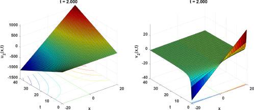
Fig.1 Asymptotic nature of and with and . |

Fig.2 Bell-shaped profiles of the expressions and with constant . |

Fig.3 Bright and dark solitons for and at arbitrary constant . |
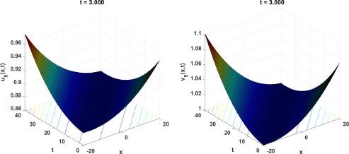
Fig.4 Parabolic profiles of the and taking . |
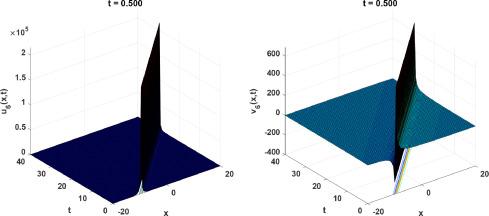
Fig.5 Bright and kink profiles of the solutions represented as and with choice of . |
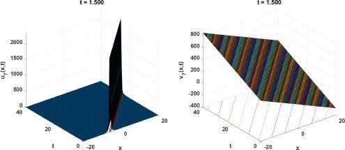
Fig.6 Bright soliton for and with . |
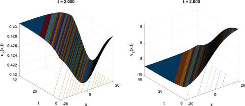
Fig.7 Kink profile of the and with . |
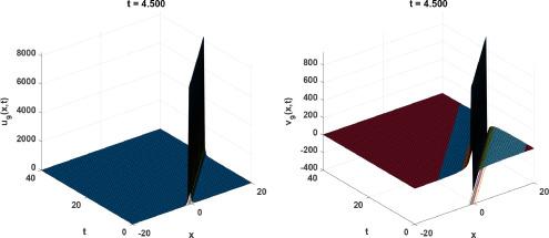
Fig.8 Bright and kink profiles for and with . |

Fig.9 Bright and kink soliton profile for and at . |

Fig.10 Periodic nature of and choosing . |

Fig.11 Periodic of and with . |
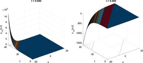
Fig.12 Asymptotic nature profiles of and taking . |
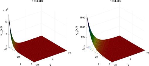
Fig.13 Asymptotic of and treating . |
Availability of data and materials
Data sharing does not apply to this article.
Funding
Not applicable.
Declaration of Competing Interest
The authors declare that they have no known competing financial interests or personal relationships that could have appeared to influence the work reported in this paper.
