Lump and travelling wave solutions of a (3 + 1)-dimensional nonlinear evolution equation

Kalim U. Tariq; Raja Nadir Tufail

doi:10.1016/j.joes.2022.04.018

Journal of Ocean Engineering and Science >

2024 , Vol. 9 >Issue 2: 164 - 172

DOI: https://doi.org/10.1016/j.joes.2022.04.018

Research article

Lump and travelling wave solutions of a (3 + 1)-dimensional nonlinear evolution equation

Kalim U. Tariq ^,^* ,
Raja Nadir Tufail

Expand

Department of Mathematics, Mirpur University of Science and Technology, Mirpur, AJK 10250, Pakistan

^*E-mail address: kalimulhaq@must.edu.pk (K.U. Tariq).

Received date: 2022-02-27

Revised date: 2022-04-02

Accepted date: 2022-04-21

Online published: 2022-05-06

Fold

Abstract

In this paper, the (3+1 )-dimensional nonlinear evolution equation is studied analytically. The bilinear form of given model is achieved by using the Hirota bilinear method. As a result, the lump waves and collisions between lumps and periodic waves, the collision among lump wave and single, double-kink soliton solutions as well as the collision between lump, periodic, and single, double-kink soliton solutions for the given model are constructed. Furthermore, some new traveling wave solutions are developed by applying the exp(âˆ’Ï•(Î¾)) expansion method. The 3D, 2D and contours plots are drawn to demonstrate the nature of the nonlinear model for setting appropriate set of parameters. As a result, a collection of bright, dark, periodic, rational function and elliptic function solutions are established. The applied strategies appear to be more powerful and efficient approaches to construct some new traveling wave structures for various contemporary models of recent era.

Highlights

● The Hirota bilinear method and the $\exp (- ϕ (ξ))$ expansion technique are used to generate some new solitary wave solutions.

● The collision among lump wave and single, double-kink soliton solutions as well as the collision between lump, periodic, and single, double-kink soliton solutions of the given model are also constructed.

Key words： The Hirota bilinear method; Lump wave solution; Travelling wave solution; Exp(−φ(ξ)) expansion technique

Cite this article

Kalim U. Tariq , Raja Nadir Tufail . Lump and travelling wave solutions of a (3 + 1)-dimensional nonlinear evolution equation[J]. Journal of Ocean Engineering and Science, 2024 , 9(2) : 164 -172 . DOI: 10.1016/j.joes.2022.04.018

1. Introduction

Many phenomena in science and engineering are expressed in the form of nonlinear evolution equations (NLEEs). In the last several decades, the study of nonlinear wave structures is becoming one of the dominant eras of contemporary research. In the presence of solitary waves, the nonlinear evolution models are utilized to simulate the effect of surface for deep water and weakly nonlinear dispersive long waves. Therefore, the exact solutions of such models play a vital role of study of dynamical structures and further properties of physical phenomenon occurring in numerous fields of study, such as electromagnetic theory, fluid motion, nuclear physics, optic fibres, physical chemistry, energy physics, compound physics and fluid mechanics [1], [2], [3], [4], [5], [6], [7], [8], [9], [10], [11], [12], [13].

In the soliton theory, the solitary wave interacts with one other without losing amplitude or velocity. Their identities and forms, for example, do not change as a result of their reciprocal interactions. Furthermore, the newly developed solutions and their graphical representations demonstrate various dynamical patterns of solitary waves, which is critical to develop a pre-eminent understanding about NLEEs emerging in diversified disciplines of science and engineering. In literature, a number of travelling wave solutions have been computed with the aid of the latest computing tools such as Mathematica, Maple or Matlab [14], [15], [16], [17], [18], [19], [20], [21].

There are several approaches for finding their exact solutions, including the extended simple equation method [22], the logistic equation method [23], the Kudryashov method [24], the direct perturbation method [25], the extended modified auxiliary equation mapping method [26], [27], the inverse scattering method [28], [29], the

ϕ^{6}

-model expansion method [30], [31], the

\exp (- ϕ (ξ))

expansion method [32], the tanh method [33], [34], the Hirota bilinear method [35], [36], [37], the exp-function method [38], [39], the generalized exponential rational function method [40], [41], the Darboux transformation [42], the Bäcklund transformation [43], [44], the residual power series method [45], the homogeneous balance method [46], [47], the modified extended direct algebraic method [48], the Lie group method [49], [50] and the variable separation method [51], [52].

The (

3 + 1

)-dimensional NLEE is a new integrable equation that can be used to explore shallow-water waves and short waves in nonlinear dispersive models. This model was initially used to explore the algebraic geometrical solutions [53] and with the help of the (1 + 1)-dimensional AKNS model, it can be reduced into a systems of solvable ordinary differential equations. In [54], the rogue waves and the rational solutions were obtained. An N-fold Darboux transformation was used to generate the complexiton solution, resonant solution and N-soliton solution [55]. The Hirota bilinear approach was used to create the N-soliton solution and its Wronskian form [56], [57]. The collision of first-order lump and line solitons to the considered model are constructed in Chen et al. [58], Tang et al. [59]. The multiple soliton solutions and a variety of traveling wave solutions of the equation are produced in Wazwaz [60], 61], 62]. The exact solutions, Bäcklund transformation and Bilinear representation were acquired in Liu and Liu [63].

In this work, we study the following (

3 + 1

)-dimensional nonlinear evolution equation [63]

(1)

\begin{matrix} 3 g_{x z} - {(2 g_{t} + g_{x x x} - 2 g g_{x})}_{y} + 2 {(g_{x} \partial_{x}^{- 1} g_{y})}_{x} = 0, \end{matrix}

where

\partial_{x}^{- 1}

represents integral operator of x and is defined as

(2)

\begin{matrix} (\partial_{x}^{- 1} f) (x) = \int_{- \infty}^{x} f (t) d t . \end{matrix}

In recent decades, many powerful approaches for completely integrable evolution equations have been developed and applied. Such NLEEs offer a wide range of applications in ocean engineering, which have been studied in various ways. There are a number of intriguing approaches for obtaining their exact solutions, such as Lie symmetry technique [64], two variable (

G^{'} / G

1 / G

)-expansion method [65], simplified Hirota's method [66], modified simple equation method [67], conservation laws [67], Riccati-Bernoulli sub-ODE method [68], and Bäcklund transformation [68], generalized exponential rational function method [69], generalized Kudryashov method [69], Lie group method [70] and exp-function method [71].

2. The bilinear form of (1)

The following transformation is used to produce the bilinear form of (1)

(3)

g = - 3 {[l n F]}_{x x} .

As a result, we obtain the bilinear form shown below

\begin{matrix} (D_{x}^{3} D_{y} + 2 D_{t} D_{y} - 3 D_{x} D_{z}) F . F = 0, \end{matrix}

where the D-operator [72] is defined as

\begin{matrix} D_{x}^{r} D_{t}^{s} (a . b) = {(\frac{\partial}{\partial x} - \frac{\partial}{\partial x^{'}})}^{r} {(\frac{\partial}{\partial t} - \frac{\partial}{\partial t^{'}})}^{s} \times a (x, t) . b (x^{'}, t^{'}) | x = x^{'}, t = t^{'} . \end{matrix}

Therefore, we attain

(4)

\begin{matrix} F_{x x x y} F - 3 F_{x x y} F_{x} + 3 F_{x y} F_{x x} - F_{y} F_{x x x} + 2 (F_{y t} F - F_{y} F_{t}) \\ - 3 (F_{x z} F - F_{x} F_{z}) = 0, \end{matrix}

clearly if F fulfils (1), then

g = - 3 {[l n F]}_{x x}

gives the solution of given model (1) directly.

3. The main results

In this part, various symbolic structures (mostly drawn from Ghanbari [73]) are used to construct the analytical solution of the equation.

3.1. Collision among lump wave and strip soliton

In this subsection, we consider the function as follows

(5)

\begin{matrix} F = μ_{0} + μ_{1} ω_{1}^{2} + μ_{2} ω_{2}^{2} + μ_{3} e^{ω_{3}}, \end{matrix}

where

\begin{matrix} ω_{1} & = & α_{0} + α_{1} x + α_{2} y + α_{3} z + α_{4} t, \\ ω_{2} & = & β_{0} + β_{1} x + β_{2} y + β_{3} z + β_{4} t, \\ ω_{3} & = & γ_{0} + γ_{1} x + γ_{2} y + γ_{3} z + γ_{4} t, \end{matrix}

here

α_{i}, β_{i}, γ_{i}

's are the unknown constants. Throughout this paper, these definitions for

ω_{1}

ω_{2}

, and

ω_{3}

are still valid.

Inserting (5) into (4), we obtain a set of equations involving various parameters. After solving this system with the help of some computing tool like Mathematica, we acquire the following results:

Case 1:

\begin{matrix} γ_{4} = - \frac{γ_{1}^{3} γ_{2} - 3 γ_{1} γ_{3}}{2 γ_{2}}, μ_{1} = 0, μ_{2} = 0, \end{matrix}

where

γ_{0}

γ_{1}

γ_{2}

γ_{3}

μ_{0}

μ_{3}

are free parameters. So using these parameters, Eq. (5) becomes

(6)

\begin{matrix} F = μ_{0} + μ_{3} \exp (γ_{0} + γ_{1} x + γ_{2} y + γ_{3} z - \frac{(γ_{1}^{3} γ_{2} - 3 γ_{1} γ_{3}) t}{2 γ_{2}}) . \end{matrix}

Using (6) along with (3), we obtain the solution

g_{1} (x, y, z, t)

of (1).

Case 2:

\begin{matrix} μ_{3} = 0, α_{4} = \frac{3 (α_{3} β_{1} β_{2} μ_{2} - α_{2} β_{1} β_{3} μ_{2} + α_{1} β_{2} β_{3} μ_{2} + α_{1} α_{2} α_{3} μ_{1})}{2 (α_{2}^{2} μ_{1} + β_{2}^{2} μ_{2})}, \\ β_{4} = \frac{3 (α_{2} α_{3} β_{1} μ_{1} - α_{1} α_{3} β_{2} μ_{1} + α_{1} α_{2} β_{3} μ_{1} + β_{1} β_{2} β_{3} μ_{2})}{2 (α_{2}^{2} μ_{1} + β_{2}^{2} μ_{2})}, \\ μ_{0} = \frac{(α_{2}^{2} μ_{1} + β_{2}^{2} μ_{2}) (α_{1}^{2} β_{1} β_{2} μ_{1} μ_{2} + α_{2} α_{1} β_{1}^{2} μ_{1} μ_{2} + α_{2} α_{1}^{3} μ_{1}^{2} + β_{1}^{3} β_{2} μ_{2}^{2})}{μ_{1} μ_{2} (α_{2} β_{1} - α_{1} β_{2}) (α_{2} β_{3} - α_{3} β_{2})}, \end{matrix}

where

α_{0}

α_{1}

α_{2}

α_{3}

β_{0}

β_{1}

β_{2}

β_{3}

μ_{1}

μ_{2}

are free parameters. Using all these obtained values along with (5) and then utilizing (3), we get the solution

g_{2} (x, y, z, t)

of (1).

Case 3:

\begin{matrix} α_{2} & = & \frac{α_{3} β_{2}}{β_{3}}, α_{4} = \frac{3 α_{1} β_{3}}{2 β_{2}}, \\ β_{4} & = & \frac{3 β_{1} β_{3}}{2 β_{2}}, μ_{2} = - \frac{α_{1}^{2} μ_{1}}{β_{1}^{2}}, μ_{3} = 0, \end{matrix}

where

α_{0}

α_{1}

α_{3}

β_{0}

β_{1}

β_{2}

β_{3}

μ_{0}

μ_{1}

are free parameters. So using these parameters, Eq. (5) becomes

(7)

\begin{matrix} F & = & μ_{0} + μ_{1} {(\frac{3 α_{1} β_{3} t}{2 β_{2}} + \frac{α_{3} β_{2} y}{β_{3}} + α_{1} x + α_{3} z + α_{0})}^{2} \\ - \frac{α_{1}^{2} μ_{1} {(\frac{3 β_{1} β_{3} t}{2 β_{2}} + β_{1} x + β_{2} y + β_{3} z + β_{0})}^{2}}{β_{1}^{2}} . \end{matrix}

Using (7) along with (3), we acquire the solution

g_{3} (x, y, z, t)

of (1).

Case 4:

\begin{matrix} α_{2} & = & \frac{α_{1} β_{2}}{β_{1}}, α_{4} = \frac{3 α_{3} β_{1}^{2} + 3 α_{1} β_{3} β_{1} - 2 α_{1} β_{2} β_{4}}{2 β_{1} β_{2}}, \\ μ_{2} & = & - \frac{α_{1}^{2} μ_{1}}{β_{1}^{2}}, μ_{0} = 0, μ_{3} = 0, \end{matrix}

where

α_{0}

α_{1}

α_{3}

β_{0}

β_{1}

β_{2}

β_{3}

β_{4}

μ_{1}

are free parameters. So using these parameters, Eq. (5) becomes

(8)

\begin{matrix} F = {(\frac{t (3 α_{3} β_{1}^{2} + 3 α_{1} β_{3} β_{1} - 2 α_{1} β_{2} β_{4})}{2 β_{1} β_{2}} + \frac{α_{1} β_{2} y}{β_{1}} + α_{1} x + α_{3} z + α_{0})}^{2} μ_{1} \\ - \frac{α_{1}^{2} μ_{1} {(β_{4} t + β_{1} x + β_{2} y + β_{3} z + β_{0})}^{2}}{β_{1}^{2}} . \end{matrix}

Using (8) along with (3), we attain the solution

g_{4} (x, y, z, t)

of (1).

3.2. Collision between lump wave and double stripes soliton

In this part, we obtain the following function

(9)

\begin{matrix} F = μ_{0} + μ_{1} ω_{1}^{2} + μ_{2} ω_{2}^{2} + μ_{3} \cosh (ω_{3}) . \end{matrix}

Putting (9) into (4), we obtain a set of equations involving various parameters. After solving this system with the help of some computing tool like Mathematica, we get the following results:

Case 1:

\begin{matrix} γ_{4} = - \frac{4 γ_{1}^{3} γ_{2} - 3 γ_{1} γ_{3}}{2 γ_{2}}, μ_{0} = 0, μ_{1} = 0, μ_{2} = 0, \end{matrix}

where

γ_{0}

γ_{1}

γ_{2}

γ_{3}

μ_{3}

are free parameters. So using these parameters, Eq. (9) becomes

(10)

\begin{matrix} F = μ_{3} \cosh (- \frac{(4 γ_{1}^{3} γ_{2} - 3 γ_{1} γ_{3}) t}{2 γ_{2}} + γ_{1} x + γ_{2} y + γ_{3} z + γ_{0}) . \end{matrix}

Using (10) along with (3), we acquire the solution

g_{5} (x, y, z, t)

of (1).

Case 2:

\begin{matrix} α_{2} & = & \frac{β_{1} β_{3} μ_{0} μ_{2}}{α_{1} μ_{1} (α_{1}^{2} μ_{1} + β_{1}^{2} μ_{2})}, \\ α_{4} & = & \frac{3 α_{1} (α_{1}^{2} μ_{1} + β_{1}^{2} μ_{2}) (α_{1} α_{3} μ_{1} - β_{1} β_{3} μ_{2})}{2 β_{1} β_{3} μ_{0} μ_{2}}, \\ μ_{3} & = & 0, β_{2} = 0, β_{4} \\ = & \frac{3 α_{1} μ_{1} (α_{3} β_{1} + α_{1} β_{3}) (α_{1}^{2} μ_{1} + β_{1}^{2} μ_{2})}{2 β_{1} β_{3} μ_{0} μ_{2}}, \end{matrix}

where

α_{0}

α_{1}

α_{3}

β_{0}

β_{1}

β_{2}

β_{3}

μ_{0}

μ_{1}

μ_{2}

are free parameters. Using all these obtained values along with (9) and then utilizing (3), we attain the solution

g_{6} (x, y, z, t)

of (1).

Case 3:

\begin{matrix} α_{2} & = & 0, α_{4} = \frac{3 β_{1} μ_{2} (α_{3} β_{1} + α_{1} β_{3}) (α_{1}^{2} μ_{1} + β_{1}^{2} μ_{2})}{2 α_{1} α_{3} μ_{0} μ_{1}}, μ_{3} = 0, \\ β_{2} & = & \frac{α_{1} α_{3} μ_{0} μ_{1}}{β_{1} μ_{2} (α_{1}^{2} μ_{1} + β_{1}^{2} μ_{2})}, \\ β_{4} & = & - \frac{3 β_{1} (α_{1}^{2} μ_{1} + β_{1}^{2} μ_{2}) (α_{1} α_{3} μ_{1} - β_{1} β_{3} μ_{2})}{2 α_{1} α_{3} μ_{0} μ_{1}}, \end{matrix}

where

α_{0}

α_{1}

α_{3}

β_{0}

β_{1}

β_{3}

μ_{0}

μ_{1}

μ_{2}

are free parameters. Using all these obtained values along with (9) and then utilizing (3), we obtain the solution

g_{7} (x, y, z, t)

of (1).

Case 4:

\begin{matrix} μ_{0} = 0, μ_{1} = 0, μ_{2} = 0, γ_{3} = \frac{2 (2 γ_{2} γ_{1}^{3} + γ_{2} c_{4})}{3 γ_{1}}, \end{matrix}

where

γ_{0}

γ_{1}

γ_{2}

γ_{4}

μ_{3}

are free parameters. So using these parameters, Eq. (9) becomes

(11)

\begin{matrix} F = μ_{3} \cosh (γ_{4} t + γ_{1} x + γ_{2} y + \frac{2 (2 γ_{2} γ_{1}^{3} + γ_{2} γ_{4}) z}{3 γ_{1}} + γ_{0}) . \end{matrix}

Using (11) along with (3), we get the solution

g_{8} (x, y, z, t)

of (1).

3.3. Collision among lump and periodic waves

In this case, we attain the function

F

as follows

(12)

\begin{matrix} F = μ_{0} + μ_{1} ω_{1}^{2} + μ_{2} ω_{2}^{2} + μ_{3} \cos (ω_{3}) . \end{matrix}

Inserting (12) into (4), we obtain a set of equations involving various parameters. After solving this system with the help of some computing tool like Mathematica, we acquire the following results:

Case 1:

\begin{matrix} γ_{4} = \frac{γ_{1} (4 γ_{2} γ_{1}^{2} + 3 γ_{3})}{2 γ_{2}}, μ_{0} = 0, μ_{1} = 0, μ_{2} = 0, \end{matrix}

where

γ_{0}

γ_{1}

γ_{2}

γ_{3}

μ_{3}

are free parameters. So using these parameters, Eq. (12) becomes

(13)

\begin{matrix} F = μ_{3} \cos (\frac{γ_{1} (4 γ_{2} γ_{1}^{2} + 3 γ_{3}) t}{2 γ_{2}} + γ_{1} x + γ_{2} y + γ_{3} z + γ_{0}) . \end{matrix}

Using (13) along with (3), we acquire the solution

g_{9} (x, y, z, t)

of (1).

3.4. Collision between lump wave and double stripes soliton

Finally, we obtain the general structure stated as

(14)

\begin{matrix} F = μ_{0} + μ_{1} ω_{1}^{2} + μ_{2} \cosh (ω_{2}) + μ_{3} \cos (ω_{3}) . \end{matrix}

Inserting (14) into (4), we obtain a set of equations involving various parameters. After solving this system with the help of some computing tool like Mathematica, we attain the following results:

Case 1:

\begin{matrix} β_{2} & = & \frac{β_{1} β_{3} + γ_{1} γ_{3}}{β_{1} (β_{1}^{2} + γ_{1}^{2})}, \\ β_{4} & = & \frac{- 4 β_{1}^{3} γ_{1} γ_{3} + 3 β_{3} β_{1}^{2} γ_{1}^{2} - β_{1}^{4} β_{3}}{2 (β_{1} β_{3} + γ_{1} γ_{3})}, μ_{0} = 0, \\ γ_{2} & = & \frac{- β_{1} β_{3} - γ_{1} γ_{3}}{γ_{1} (β_{1}^{2} + γ_{1}^{2})}, \\ γ_{4} & = & \frac{4 β_{1} β_{3} γ_{1}^{3} - 3 β_{1}^{2} γ_{3} γ_{1}^{2} + γ_{3} γ_{1}^{4}}{2 (β_{1} β_{3} + γ_{1} γ_{3})}, μ_{1} = 0, \end{matrix}

where

β_{0}

β_{1}

β_{3}

γ_{0}

γ_{1}

γ_{3}

μ_{2}

μ_{3}

are free parameters.

Using all these obtained values along with (14) and then utilizing (3), we acquire the solution

g_{10} (x, y, z, t)

of (1).

4. Travelling-wave solutions for Eq. (1)

Now, we will obtain the exact traveling wave solutions for (1) using

\exp (- ϕ (ξ))

expansion technique. Firstly, substituting

(15)

g (x, y, z, t) = v_{x},

in (1) and utilizing the boundary condition

g_{y} | x \to - \infty = 0

, we get

(16)

3 v_{x x z} - {(2 v_{x t} + v_{x x x x} - 2 v_{x} v_{x x})}_{y} + 2 {(v_{x x} v_{x y})}_{x} = 0

Next, we obtain the transformation stated as

(17)

v (x, y, z, t) = Ω (ξ), ξ = α x + β y + γ z + λ t,

here

α, β, γ

are constants and

λ

is the speed of the wave. We use the transformation (17) in (16) to get an ordinary differential equation as

(18)

\begin{matrix} - α^{4} β Ω^{(5)} (ξ) + (3 α^{2} γ - 2 α β λ) Ω^{(3)} (ξ) \\ + 4 α^{3} β (Ω^{″} {(ξ)}^{2} + Ω^{(3)} (ξ) Ω^{'} (ξ)) = 0 . \end{matrix}

Integrating it twice, we get

(19)

- α^{4} β Ω^{(3)} (ξ) + (3 α^{2} γ - 2 α β λ) Ω^{^{'}} (ξ) + 2 α^{3} β Ω^{^{'}} {(ξ)}^{2} .

Using the considered method, we assume the solution of (19) as follows:

(20)

Ω (ξ) = \sum_{i = 0}^{M} A_{i} {(e x p (- ϕ (ξ)))}^{i},

here

A_{i} (0 \leq i \leq M)

are parameters, and

(21)

ϕ^{'} (ξ) = e x p (- ϕ (ξ)) + e x p (ϕ (ξ)) P + Q .

Group 1:

Q^{2} - 4 P > 0, P \neq 0

(22)

ϕ (ξ) = \ln (\frac{- \sqrt{Q^{2} - 4 P} \tanh (\frac{1}{2} (C + ξ) \sqrt{Q^{2} - 4 P}) - Q}{2 P}),

(23)

\begin{matrix} ϕ (ξ) = \ln (\frac{(- \sqrt{Q^{2} - 4 P}) \coth (\frac{1}{2} (C + ξ) \sqrt{Q^{2} - 4 P}) - Q}{2 P}), \end{matrix}

where C is an integration constant.

Group 2:

Q^{2} - 4 P < 0, P \neq 0

(24)

ϕ (ξ) = \ln (\frac{\sqrt{4 P - Q^{2}} \tan (\frac{1}{2} (C + ξ) \sqrt{4 P - Q^{2}}) - Q}{2 P}),

(25)

\begin{matrix} ϕ (ξ) = \ln (\frac{\sqrt{4 P - Q^{2}} \cot (\frac{1}{2} (C + ξ) \sqrt{4 P - Q^{2}}) - Q}{2 P}) . \end{matrix}

Group 3:

Q^{2} - 4 P > 0

P = 0

Q \neq 0

(26)

ϕ (ξ) = - \ln (\frac{Q}{e^{Q (C + ξ)} - 1}) .

Group 4:

Q^{2} - 4 P = 0

P \neq 0

Q \neq 0

(27)

ϕ (ξ) = \ln (- \frac{2 (Q (C + ξ) + 2)}{Q^{2} (C + ξ)}) .

Group 5:

Q^{2} - 4 P = 0

P = 0

Q = 0

(28)

ϕ (ξ) = \ln (C + ξ) .

Balancing

Ω^{(3)} (ξ)

and

Ω^{^{'}} {(ξ)}^{2}

in (19), we obtain

M = 1

. Therefore, Eq. (20) can be stated as follows

(29)

Ω (ξ) = A_{0} + A_{1} e^{- ϕ (ξ)} .

Putting (29) along with (21) into (19), we obtain an algebraic system of equations given as follows:

\begin{matrix} 6 α^{4} A_{1} β + 2 α^{3} A_{1}^{2} β = 0, \\ 12 α^{4} A_{1} β Q + 4 α^{3} A_{1}^{2} β Q = 0, \\ α^{4} A_{1} β Q^{3} + 8 α^{4} A_{1} β P Q + 4 α^{3} A_{1}^{2} β P Q - 3 α^{2} A_{1} γ Q + 2 α A_{1} β λ Q = 0, \\ 2 α^{4} A_{1} β P^{2} + α^{4} A_{1} β P Q^{2} + 2 α^{3} A_{1}^{2} β P^{2} - 3 α^{2} A_{1} γ P + 2 α A_{1} β λ P = 0, \\ 8 α^{4} A_{1} β P + 7 α^{4} A_{1} β Q^{2} + 4 α^{3} A_{1}^{2} β P + 2 α^{3} A_{1}^{2} β Q^{2} - 3 α^{2} A_{1} γ + 2 α A_{1} β λ = 0, \end{matrix}

We obtain the following result by solving this system:

(30)

A_{1} = - 3 α, λ = - \frac{- 4 α^{3} β P + α^{3} β Q^{2} - 3 α γ}{2 β} .

Therefore, using these parameters we attain the following solutions for the given model:

Group 1:

Q^{2} - 4 P > 0, P \neq 0

(31)

\begin{matrix} v (x, y, z, t) = A_{0} - \frac{6 α P}{- \sqrt{Q^{2} - 4 P} \tanh (\frac{1}{2} \sqrt{Q^{2} - 4 P} (C + ξ)) - Q}, \end{matrix}

inserting (31) into (15), we attain the solution as

(32)

\begin{matrix} g_{11} (x, y, z, t) = - \frac{3 α^{2} P (Q^{2} - 4 P) {sech}^{2} (\frac{1}{2} \sqrt{Q^{2} - 4 P} (C + ξ))}{{(- \sqrt{Q^{2} - 4 P} \tanh (\frac{1}{2} \sqrt{Q^{2} - 4 P} (C + ξ)) - Q)}^{2}}, \end{matrix}

similarly

(33)

\begin{matrix} v (x, y, z, t) = A_{0} - \frac{6 α P}{- \sqrt{Q^{2} - 4 P} \coth (\frac{1}{2} (C + ξ) \sqrt{Q^{2} - 4 P}) - Q}, \end{matrix}

inserting (33) into (15), we get the solution as

(34)

\begin{matrix} g_{12} (x, y, z, t) = \frac{3 α^{2} P (Q^{2} - 4 P) {csch}^{2} (\frac{1}{2} \sqrt{Q^{2} - 4 P} (C + ξ))}{{(- \sqrt{Q^{2} - 4 P} \coth (\frac{1}{2} \sqrt{Q^{2} - 4 P} (C + ξ)) - Q)}^{2}}, \end{matrix}

where

ξ = - \frac{t (- 4 α^{3} β P + α^{3} β Q^{2} - 3 α γ)}{2 β} + α x + β y + γ z

Group 2:

Q^{2} - 4 P < 0, P \neq 0

(35)

\begin{matrix} v (x, y, z, t) = A_{0} - \frac{6 α P}{\sqrt{4 P - Q^{2}} \tan (\frac{1}{2} (C + ξ) \sqrt{4 P - Q^{2}}) - Q}, \end{matrix}

inserting (35) into (15), we obtain the solution as

(36)

\begin{matrix} g_{13} (x, y, z, t) = \frac{3 α^{2} P (4 P - Q^{2}) \sec^{2} (\frac{1}{2} \sqrt{4 P - Q^{2}} (C + ξ))}{{(\sqrt{4 P - Q^{2}} \tan (\frac{1}{2} \sqrt{4 P - Q^{2}} (C + ξ)) - Q)}^{2}}, \end{matrix}

similarly

(37)

\begin{matrix} v (x, y, z, t) = A_{0} - \frac{6 α P}{\sqrt{4 P - Q^{2}} \cot (\frac{1}{2} (C + ξ) \sqrt{4 P - Q^{2}}) - Q}, \end{matrix}

inserting (37) into (15), we acquire the solution as

(38)

\begin{matrix} g_{14} (x, y, z, t) = - \frac{3 α^{2} P (4 P - Q^{2}) \csc^{2} (\frac{1}{2} \sqrt{4 P - Q^{2}} (C + ξ))}{{(\sqrt{4 P - Q^{2}} \cot (\frac{1}{2} \sqrt{4 P - Q^{2}} (C + ξ)) - Q)}^{2}}, \end{matrix}

where

ξ = - \frac{t (- 4 α^{3} β P + α^{3} β Q^{2} - 3 α γ)}{2 β} + α x + β y + γ z

Group 3:

Q^{2} - 4 P > 0

P = 0

Q \neq 0

(39)

\begin{matrix} v (x, y, z, t) \\ = A_{0} - \frac{3 α Q}{\exp (Q (C - \frac{t (- 4 α^{3} β P + α^{3} β Q^{2} - 3 α γ)}{2 β} + α x + β y + γ z)) - 1}, \end{matrix}

inserting (39) into (15), we obtain the solution as

(40)

\begin{matrix} g_{15} (x, y, z, t) \\ = \frac{3 α^{2} Q^{2} \exp (Q (C - \frac{t (- 4 α^{3} β P + α^{3} β Q^{2} - 3 α γ)}{2 β} + α x + β y + γ z))}{{(\exp (Q (C - \frac{t (- 4 α^{3} β P + α^{3} β Q^{2} - 3 α γ)}{2 β} + α x + β y + γ z)) - 1)}^{2}} . \end{matrix}

Group 4:

Q^{2} - 4 P = 0

P \neq 0

Q \neq 0

(41)

\begin{matrix} v (x, y, z, t) \\ = A_{0} + \frac{3 α Q^{2} (C - \frac{t (- 4 α^{3} β P + α^{3} β Q^{2} - 3 α γ)}{2 β} + α x + β y + γ z)}{2 (Q (C - \frac{t (- 4 α^{3} β P + α^{3} β Q^{2} - 3 α γ)}{2 β} + α x + β y + γ z) + 2)}, \end{matrix}

inserting (41) into (15), we acquire the solution as

(42)

\begin{matrix} g_{16} (x, y, z, t) \\ = - \frac{3 α^{2} Q^{3} (C - \frac{t (- 4 α^{3} β P + α^{3} β Q^{2} - 3 α γ)}{2 β} + α x + β y + γ z)}{2 {(Q (C - \frac{t (- 4 α^{3} β P + α^{3} β Q^{2} - 3 α γ)}{2 β} + α x + β y + γ z) + 2)}^{2}} . \end{matrix}

Group 5:

Q^{2} - 4 P = 0

P = 0

Q = 0

(43)

\begin{matrix} v (x, y, z, t) = A_{0} - \frac{3 α}{C - \frac{t (- 4 α^{3} β P + α^{3} β Q^{2} - 3 α γ)}{2 β} + α x + β y + γ z}, \end{matrix}

inserting (43) into (15), we attain the solution as

(44)

\begin{matrix} g_{17} (x, y, z, t) = \frac{3 α^{2}}{{(C - \frac{t (- 4 α^{3} β P + α^{3} β Q^{2} - 3 α γ)}{2 β} + α x + β y + γ z)}^{2}} . \end{matrix}

5. Discussion and results

This section displays graphical illustrations of the (

3 + 1

)-dimensional NLEE. For the suitable values of the constants involved, multiple profiles of the resultant solutions have been shown. For a given set of values, a variety of bright, dark, periodic, and singular bell-shaped solitons are shown. Fig. 1 shows the behaviour of solution

| g_{1} (x, y, z, t) |

for the values of the constants

γ_{0} = 0.7

γ_{1} = 0.5

γ_{2} = 0.75

γ_{3} = - 0.25

μ_{0} = 0.8

μ_{3} = 0.6

and it represents a bright soliton solution. Similarly, Figs. 2, 4, 6, 8, 9 and 12 also represent the bright soliton solutions for the appropriate values of the parameters involving. Fig. 3 represents the singular bell shaped solution for the values of constants

α_{0} = 0.5

α_{1} = 0.4

α_{3} = - 0.6

β_{0} = 0.55

β_{1} = 0.7

β_{2} = 0.56

β_{3} = 0.4

β_{4} = 0.3

μ_{1} = 0.5

. Also, the Figs. 11, 13 and 14 represent the singular bell shaped solutions for the appropriate values of the parameters involving. Singularities can exist anywhere, and they're surprisingly abundant in physicists' mathematics for understanding the universe. Fig. 5 represents the dark soliton solution for the values of the parameters

β_{0} = 0.15

β_{1} = 0.12

β_{3} = 0.15

α_{0} = 0.1

α_{1} = 0.12

α_{3} = 0.15

μ_{0} = 0.4

μ_{1} = 0.5

μ_{2} = 0.6

. Figs. 7 and 10 illustrate the periodic solitary waves solutions for the various values of the parameters involved. To better understand the behaviour of solutions, 3D, contour and 2D graphs of attained solutions with various parameter values are shown.

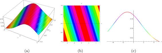
View original graphic|Download|PPT slide

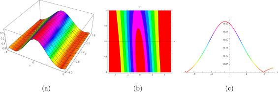
Fig.1 Profiles of the solution $| g_{1} (x, y, z, t) |$ of (1) for $γ_{0} = 0.7$ , $γ_{1} = 0.5$ , $γ_{2} = 0.75$ , $γ_{3} = - 0.25$ , $μ_{0} = 0.8$ , $μ_{3} = 0.6$ .

View original graphic|Download|PPT slide

Fig.2 Profiles of the solution $| g_{2} (x, y, z, t) |$ of (1) for $α_{0} = - 0.5$ , $α_{1} = 0.55$ , $α_{2} = 0.75$ , $α_{3} = 0.5$ , $β_{0} = 0.6$ , $β_{1} = - 0.5$ , $β_{2} = 0.4$ , $β_{3} = 0.25$ , $μ_{0} = 0.5, μ_{1} = 0.6$ , $μ_{2} = 0.7$ .

View original graphic|Download|PPT slide

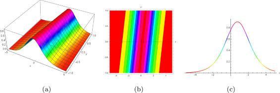
Fig.3 Profiles of the solution $| g_{4} (x, y, z, t) |$ of (1) for $α_{0} = 0.5$ , $α_{1} = 0.4$ , $α_{3} = - 0.6$ , $β_{0} = 0.55$ , $β_{1} = 0.7$ , $β_{2} = 0.56$ , $β_{3} = 0.4$ , $β_{4} = 0.3$ , $μ_{1} = 0.5$ .

View original graphic|Download|PPT slide

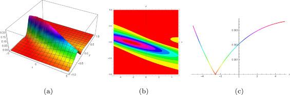
Fig.4 Profiles of the solution $| g_{5} (x, y, z, t) |$ of (1) for $γ_{0} = 0.25$ , $γ_{1} = 0.55$ , $γ_{2} = - 0.3$ , $γ_{3} = 0.025$ .

View original graphic|Download|PPT slide

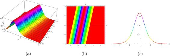
Fig.5 Profiles of the solution $| g_{7} (x, y, z, t) |$ of (1) for $β_{0} = 0.15$ , $β_{1} = 0.12$ , $β_{3} = 0.15$ , $α_{0} = 0.1$ , $α_{1} = 0.12$ , $α_{3} = 0.15$ , $μ_{0} = 0.4$ , $μ_{1} = 0.5$ , $μ_{2} = 0.6$ .

View original graphic|Download|PPT slide

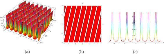
Fig.6 Profiles of the solution $| g_{8} (x, y, z, t) |$ of (1) for $γ_{0} = 1.55$ , $γ_{1} = 0.75$ , $γ_{2} = - 0.8$ , $γ_{4} = - 0.25$ .

View original graphic|Download|PPT slide

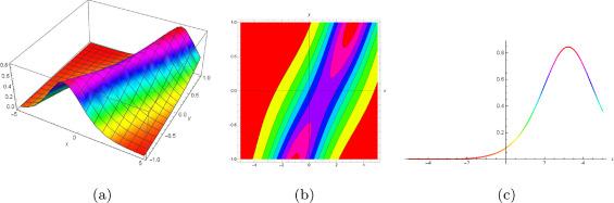
Fig.7 Profiles of the solution $| g_{9} (x, y, z, t) |$ of (1) for $γ_{0} = 0.1$ , $γ_{1} = - 2.25$ , $γ_{2} = 2.55$ , $γ_{3} = 2.25$ , $μ_{3} = 2.6$ .

View original graphic|Download|PPT slide

Fig.8 Profiles of the solution $| g_{10} (x, y, z, t) |$ of (1) for $β_{0} = 0.255$ , $β_{1} = - 0.5$ , $β_{3} = 0.255$ , $γ_{0} = 0.25$ , $γ_{1} = 0.225$ , $γ_{3} = - 0.125$ , $μ_{2} = 2.6$ , $μ_{3} = 0.25$ .

View original graphic|Download|PPT slide

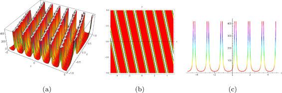
Fig.9 Profiles of the solution $| g_{11} (x, y, z, t) |$ of (1) for $α = 1.25$ , $β = 1.2$ , $γ = 1.125$ , $C = 1.35$ , $P = 0.125$ , $Q = - 1.1$ .

View original graphic|Download|PPT slide

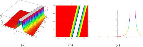
Fig.10 Profiles of the solution $| g_{12} (x, y, z, t) |$ of (1) for $α = 1.7$ , $β = 1.8$ , $γ = 1.9$ , $C = 1.35$ , $P = 1.5$ , $Q = 0.5$ .

View original graphic|Download|PPT slide

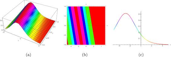
Fig.11 Profiles of the solution $| g_{13} (x, y, z, t) |$ of (1) for $α = - 0.7$ , $β = 0.85$ , $γ = 0.95$ , $C = 0.8$ , $P = - 0.56$ , $Q = 0.55$ .

View original graphic|Download|PPT slide

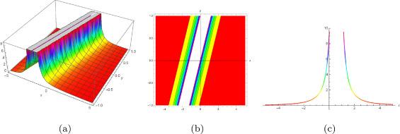
Fig.12 Profiles of the solution $| g_{14} (x, y, z, t) |$ of (1) for $α = 0.6$ , $β = 0.5$ , $γ = 0.5$ , $C = 0.6$ , $P = - 0.4$ , $Q = 0.55$ .

View original graphic|Download|PPT slide

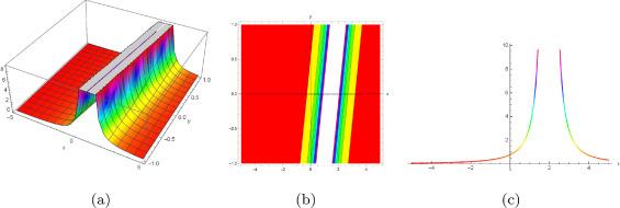
Fig.13 Profiles of the solution $| g_{15} (x, y, z, t) |$ of (1) for $α = - 0.7$ , $β = 0.85$ , $γ = 0.95$ , $C = 0.8$ , $P = 1.56$ , $Q = 0.55$ .

View original graphic|Download|PPT slide

Fig.14 Profiles of the solution $| g_{17} (x, y, z, t) |$ of (1) for $α = - 0.2$ , $β = 0.1$ , $γ = 0.3$ , $C = 0.9$ , $P = 0.5$ , $Q = 0.75$ .

6. Conclusion

In this paper, we use the Hirota bilinear approach and the

\exp (- ϕ (ξ))

expansion technique to investigate the (

3 + 1

)-dimensional NLEE. Using various sorts of functions, we were able to obtain a number of intriguing exact solutions to the given model. We were able to achieve alternative graphical interpretations of the given solutions for different sets of parameter values using Mathematica 11.0. Finally, we can say that the considered approaches can be used to explore a variety of NLEEs in mathematical physics.

Declaration of Competing Interest

The authors declare that they have no known competing financial interests or personal relationships that could have appeared to influence the work reported in this paper.

References

Publishing order | Descend order by publishing year | Descend order by cited within

[1]	A.R. Seadawy, N. Cheemaa. Mod. Phys. Lett. B,33 (18) (2019), p. 1950203 DOI: 10.1142/s0217984919502038

[2]	H. Naher, F.A. Abdullah. Appl. Math. Sci., 6 (111) (2012), pp. 5495-5512

[3]	A.M. Wazwaz. Math. Comput. Model., 40 (5-6) (2004), pp. 499-508

[4]	I. Ahmed, A.R. Seadawy, D. Lu. Phys. Scr., 94 (5) (2019), p. 055205 DOI: 10.1088/1402-4896/ab0455

[5]	N.A. Kudryashov. Optik, 183 (2019), pp. 642-649

[6]	A.M. Wazwaz. Appl. Math. Comput., 187 (2) (2007), pp. 1131-1142

[7]	Y.-L. Sun, W.-X. Ma, J.P. Yu. Appl. Math. Lett., 120 (2021), p. 107224

[8]	A.R. Seadawy, S.T.R. Rizvi, S. Ahmad, M. Younis, D. Baleanu. Open Phys., 19 (1) (2021), pp. 1-10 DOI: 10.1515/phys-2020-0224

[9]	S.T.R. Rizvi, I. Bibi, M. Younis, A. Bekir. Chin. Phys. B, 30 (1) (2021), p. 010502

[10]	M. Higazy, S. Muhammad, A. Al-Ghamdi, M.M. Khater. J. Ocean Eng. Sci. (2022)

[11]	M.M. Miah, A.R. Seadawy, H.S. Ali, M.A. Akbar. J. Ocean Eng. Sci., 5 (3) (2020), pp. 269-278

[12]	M. Durand, D. Langevin. Eur. Phys. J. E, 7 (1) (2002), pp. 35-44

[13]	N. Kudryashov. Phys. Lett. A, 155 (4-5) (1991), pp. 269-275

[14]	L.-x. Li, E.-q. Li, M.l. Wang. Appl. Math., 25 (4) (2010), pp. 454-462 DOI: 10.1007/s11766-010-2128-x

[15]	K. Hosseini, P. Mayeli, D. Kumar. J. Mod. Opt., 65 (3) (2018), pp. 361-364 DOI: 10.1080/09500340.2017.1380857

[16]	A.M. Wazwaz. Phys. Scr., 89 (9) (2014), p. 095206 DOI: 10.1088/0031-8949/89/9/095206

[17]	Z. Ivezic, S.M. Kahn, J.A. Tyson, B. Abel, E. Acosta, R. Allsman, D. Alonso, Y. AlSayyad, S.F. Anderson, J. Andrew, et al.. Astrophys. J., 873 (2) (2019), p. 111 DOI: 10.3847/1538-4357/ab042c

[18]	A. Bekir, A. Boz. Phys. Lett. A, 372 (10) (2008), pp. 1619-1625

[19]	A.D. Alruwaili, A.R. Seadawy, S.T. Rizvi, S.A.O. Beinane. Mathematics, 10 (2) (2022), p. 200 DOI: 10.3390/math10020200

[20]	A. Bekir. Phys. Lett. A, 372 (19) (2008), pp. 3400-3406

[21]	M. Osman. Waves Random Complex Media, 26 (4) (2016), pp. 434-443 DOI: 10.1080/17455030.2016.1166288

[22]	M. Khater, A. Jhangeer, H. Rezazadeh, L. Akinyemi, M.A. Akbar, M. Inc, H. Ahmad. Opt. Quantum Electron., 53 (11) (2021), pp. 1-27 DOI: 10. 3138/diaspora.21.1.2020-06-15

[23]	Z. Pinar, H. Rezazadeh, M. Eslami. Opt. Quantum Electron., 52 (12) (2020), pp. 1-16 DOI: 10.23834/isrjournal.839937

[24]	A. Zafar, M. Shakeel, A. Ali, L. Akinyemi, H. Rezazadeh. Opt. Quantum Electron., 54 (1) (2022), pp. 1-15 DOI: 10.53963/pjmr.2022.006.4

[25]	Y.-Q. Chen, Y.-H. Tang, J. Manafian, H. Rezazadeh, M. Osman. Nonlinear Dyn., 105 (3) (2021), pp. 2539-2548 DOI: 10.1007/s11071-021-06642-6

[26]	U. Akram, A.R. Seadawy, S. Rizvi, M. Younis, S. Althobaiti, S. Sayed. Results Phys., 20 (2021), p. 103725

[27]	S.T.R. Rizvi, S. Ahmad, M.F. Nadeem, M. Awais. Optik, 226 (2021), p. 165955

[28]	M.J. Ablowitz, H. Segur. Solitons and the Inverse Scattering Transform. SIAM (1981)

[29]	M.J. Ablowitz, M. Ablowitz, P. Clarkson, P.A. Clarkson. Solitons, Nonlinear Evolution Equations and Inverse Scattering. vol. 149, Cambridge University Press (1991)

[30]	A.R. Seadawy, M. Bilal, M. Younis, S. Rizvi, S. Althobaiti, M. Makhlouf. Chaos, Solitons Fractals, 144 (2021), p. 110669

[31]	A.R. Seadawy, S. Rehman, M. Younis, S. Rizvi, S. Althobaiti, M. Makhlouf. Phys. Scr., 96 (4) (2021), p. 045202 DOI: 10.1088/1402-4896/abdcf7

[32]	A.R. Seadawy, D. Lu, M.M. Khater. J. Ocean Eng. Sci., 2 (2) (2017), pp. 137-142

[33]	M. Abdelkawy, A. Bhrawy, E. Zerrad, A. Biswas. Acta Phys. Pol. A, 129 (3) (2016), pp. 278-283 DOI: 10.12693/APhysPolA.129.278

[34]	A. Bekir. Commun. Nonlinear Sci. Numer. Simul., 13 (9) (2008), pp. 1748-1757

[35]	R. Hirota. Direct Methods in Soliton Theory, Solitons, Springer (1980), pp. 157-176 DOI: 10.1007/978-3-642-81448-8_5

[36]	J. Satsuma. Hirota bilinear method for nonlinear evolution equations. Direct and Inverse Methods in Nonlinear Evolution Equations, Springer (2003), pp. 171-222 DOI: 10.1007/978-3-540-39808-0_4

[37]	M. Younis, S. Ali, S.T.R. Rizvi, M. Tantawy, K.U. Tariq, A. Bekir. Commun. Nonlinear Sci. Numer. Simul., 94 (2021), p. 105544

[38]	Y. Gurefe, E. Misirli. Comput. Math. Appl., 61 (8) (2011), pp. 2025-2030

[39]	E. Misirli, Y. Gurefe. Math. Comput. Appl.,16 (1) (2011), pp. 258-266 DOI: 10.3390/mca16010258

[40]	U. Younas, M. Younis, A.R. Seadawy, S. Rizvi, S. Althobaiti, S. Sayed. Results Phys., 20 (2021), p. 103766

[41]	F.S. Khodadad, S. Mirhosseini-Alizamini, B. GÃ¼nay, L. Akinyemi, H. Rezazadeh, M. Inc. Opt. Quantum Electron., 53 (12) (2021), pp. 1-17

[42]	X. Geng, G. He. J. Math. Phys., 51 (3) (2010), p. 033514

[43]	S. Carillo, M.L. Schiavo, C. Schiebold, et al.. SIGMA, 12 (2016), p. 087

[44]	R. Hirota, J. Satsuma. Prog. Theor. Phys.,57 (3) (1977), pp. 797-807 DOI: 10.1143/PTP.57.797

[45]	S. Rizvi, A.R. Seadawy, S. Abbas, S. Latif, S. Althobaiti. Comput. Appl. Math.,41 (1) (2022), pp. 1-18 DOI: 10.1504/ijmor.2022.10052805

[46]	E. Zayed, S.H. Ibrahim. Chin. Phys. Lett., 29 (6) (2012), p. 060201

[47]	H. Jafari, N. Kadkhoda, C.M. Khalique. Comput. Math. Appl., 64 (6) (2012), pp. 2084-2088

[48]	H. Rehman, A.R. Seadawy, M. Younis, S. Rizvi, I. Anwar, M. Baber, A. Althobaiti. Results Phys., 33 (2022), p. 105069

[49]	G.W. Bluman, S. Kumei. Symmetries and Differential Equations. vol. 81, Springer Science and Business Media (2013)

[50]	B. Bira, T.R. Sekhar, D. Zeidan. Math. Methods Appl. Sci., 41 (16) (2018), pp. 6717-6725 DOI: 10.1002/mma.5186

[51]	S.-y. Lou, L.L. Chen. J. Math. Phys., 40 (12) (1999), pp. 6491-6500

[52]	C.-Q. Dai, Y.Y. Wang. Commun. Nonlinear Sci. Numer. Simul., 19 (1) (2014), pp. 19-28

[53]	X. Geng. J. Phys. A, 36 (9) (2003), p. 2289

[54]	Zhaqilao. Phys. Lett. A, 377 (42) (2013), pp. 3021-3026

[55]	Zhaqilao Z.B. Li. Mod. Phys. Lett. B, 22 (30) (2008), pp. 2945-2966

[56]	X. Geng, Y. Ma. Phys. Lett. A, 369 (4) (2007), pp. 285-289

[57]	S.T.R. Rizvi, K. Ali, A. Bekir, B. Nawaz, M. Younis. Qual. Theory Dyn. Syst.,21 (1) (2022), pp. 1-14 DOI: 10.1504/ijmor.2022.10052805

[58]	M.-D. Chen, X. Li, Y. Wang, B. Li. Commun. Theor. Phys., 67 (6) (2017), p. 595 DOI: 10.1088/0253-6102/67/6/595

[59]	Y. Tang, S. Tao, M. Zhou, Q. Guan. Nonlinear Dyn., 89 (1) (2017), pp. 429-442 DOI: 10.1007/s11071-017-3462-9

[60]	A.M. Wazwaz. Appl. Math. Comput., 215 (4) (2009), pp. 1548-1552

[61]	A.M. Wazwaz. Math. hods Appl. Sci., 36 (3) (2013), pp. 349-357 DOI: 10.1002/mma.2600

[62]	A.M. Wazwaz. Cent. Eur. J. Eng., 4 (4) (2014), pp. 352-356

[63]	N. Liu, Y. Liu. Comput. Math. Appl., 71 (8) (2016), pp. 1645-1654

[64]	M. Niwas, S. Kumar, H. Kharbanda. J. Ocean Eng. Sci., 7 (2) (2022), pp. 188-201

[65]	M.M. Miah, H.S. Ali, M.A. Akbar, A.R. Seadawy. J. Ocean Eng. Sci., 4 (2) (2019), pp. 132-143

[66]	S. Singh, S.S. Ray. J. Ocean Eng. Sci. (2022)

[67]	A. Akbulut, M. Kaplan, M.K. Kaabar. J. Ocean Eng. Sci. (2021)

[68]	H. Esen, N. Ozdemir, A. Secer, M. Bayram. J. Ocean Eng. Sci. (2021)

[69]	S. Kumar, A. Kumar, B. Mohan. J. Ocean Eng. Sci. (2021)

[70]	S. Kumar, S. Rani. J. Ocean Eng. Sci. (2021)

[71]	L. Ravi, S.S. Ray, S. Sahoo. J. Ocean Eng. Sci., 2 (1) (2017), pp. 34-46

[72]	R. Hirota. The Direct Method in Soliton Theory. vol. 155, Cambridge University Press (2004)

[73]	B. Ghanbari. Results Phys., 29 (2021), p. 104689

Options

Outlines

模态框（Modal）标题

Abstract

Cite this article

1. Introduction

2. The bilinear form of (1)

3. The main results

3.1. Collision among lump wave and strip soliton

3.2. Collision between lump wave and double stripes soliton

3.3. Collision among lump and periodic waves

3.4. Collision between lump wave and double stripes soliton

4. Travelling-wave solutions for Eq. (1)

5. Discussion and results

Fig.1 Profiles of the solution |g1(x,y,z,t)| of (1) for γ0=0.7 , γ1=0.5 , γ2=0.75 , γ3=−0.25 , μ0=0.8 , μ3=0.6 .

Fig.2 Profiles of the solution |g2(x,y,z,t)| of (1) for α0=−0.5 , α1=0.55 , α2=0.75 , α3=0.5 , β0=0.6 , β1=−0.5 , β2=0.4 , β3=0.25 , μ0=0.5,μ1=0.6 , μ2=0.7 .

Fig.3 Profiles of the solution |g4(x,y,z,t)| of (1) for α0=0.5 , α1=0.4 , α3=−0.6 , β0=0.55 , β1=0.7 , β2=0.56 , β3=0.4 , β4=0.3 , μ1=0.5 .

Fig.4 Profiles of the solution |g5(x,y,z,t)| of (1) for γ0=0.25 , γ1=0.55 , γ2=−0.3 , γ3=0.025 .

Fig.5 Profiles of the solution |g7(x,y,z,t)| of (1) for β0=0.15 , β1=0.12 , β3=0.15 , α0=0.1 , α1=0.12 , α3=0.15 , μ0=0.4 , μ1=0.5 , μ2=0.6 .

Fig.6 Profiles of the solution |g8(x,y,z,t)| of (1) for γ0=1.55 , γ1=0.75 , γ2=−0.8 , γ4=−0.25 .

Fig.7 Profiles of the solution |g9(x,y,z,t)| of (1) for γ0=0.1 , γ1=−2.25 , γ2=2.55 , γ3=2.25 , μ3=2.6 .

Fig.8 Profiles of the solution |g10(x,y,z,t)| of (1) for β0=0.255 , β1=−0.5 , β3=0.255 , γ0=0.25 , γ1=0.225 , γ3=−0.125 , μ2=2.6 , μ3=0.25 .

Fig.9 Profiles of the solution |g11(x,y,z,t)| of (1) for α=1.25 , β=1.2 , γ=1.125 , C=1.35 , P=0.125 , Q=−1.1 .

Fig.10 Profiles of the solution |g12(x,y,z,t)| of (1) for α=1.7 , β=1.8 , γ=1.9 , C=1.35 , P=1.5 , Q=0.5 .

Fig.11 Profiles of the solution |g13(x,y,z,t)| of (1) for α=−0.7 , β=0.85 , γ=0.95 , C=0.8 , P=−0.56 , Q=0.55 .

Fig.12 Profiles of the solution |g14(x,y,z,t)| of (1) for α=0.6 , β=0.5 , γ=0.5 , C=0.6 , P=−0.4 , Q=0.55 .

Fig.13 Profiles of the solution |g15(x,y,z,t)| of (1) for α=−0.7 , β=0.85 , γ=0.95 , C=0.8 , P=1.56 , Q=0.55 .

Fig.14 Profiles of the solution |g17(x,y,z,t)| of (1) for α=−0.2 , β=0.1 , γ=0.3 , C=0.9 , P=0.5 , Q=0.75 .

6. Conclusion

Declaration of Competing Interest

References

Links

Fig.1 Profiles of the solution $| g_{1} (x, y, z, t) |$ of (1) for $γ_{0} = 0.7$ , $γ_{1} = 0.5$ , $γ_{2} = 0.75$ , $γ_{3} = - 0.25$ , $μ_{0} = 0.8$ , $μ_{3} = 0.6$ .

Fig.2 Profiles of the solution $| g_{2} (x, y, z, t) |$ of (1) for $α_{0} = - 0.5$ , $α_{1} = 0.55$ , $α_{2} = 0.75$ , $α_{3} = 0.5$ , $β_{0} = 0.6$ , $β_{1} = - 0.5$ , $β_{2} = 0.4$ , $β_{3} = 0.25$ , $μ_{0} = 0.5, μ_{1} = 0.6$ , $μ_{2} = 0.7$ .

Fig.3 Profiles of the solution $| g_{4} (x, y, z, t) |$ of (1) for $α_{0} = 0.5$ , $α_{1} = 0.4$ , $α_{3} = - 0.6$ , $β_{0} = 0.55$ , $β_{1} = 0.7$ , $β_{2} = 0.56$ , $β_{3} = 0.4$ , $β_{4} = 0.3$ , $μ_{1} = 0.5$ .

Fig.4 Profiles of the solution $| g_{5} (x, y, z, t) |$ of (1) for $γ_{0} = 0.25$ , $γ_{1} = 0.55$ , $γ_{2} = - 0.3$ , $γ_{3} = 0.025$ .

Fig.5 Profiles of the solution $| g_{7} (x, y, z, t) |$ of (1) for $β_{0} = 0.15$ , $β_{1} = 0.12$ , $β_{3} = 0.15$ , $α_{0} = 0.1$ , $α_{1} = 0.12$ , $α_{3} = 0.15$ , $μ_{0} = 0.4$ , $μ_{1} = 0.5$ , $μ_{2} = 0.6$ .

Fig.6 Profiles of the solution $| g_{8} (x, y, z, t) |$ of (1) for $γ_{0} = 1.55$ , $γ_{1} = 0.75$ , $γ_{2} = - 0.8$ , $γ_{4} = - 0.25$ .

Fig.7 Profiles of the solution $| g_{9} (x, y, z, t) |$ of (1) for $γ_{0} = 0.1$ , $γ_{1} = - 2.25$ , $γ_{2} = 2.55$ , $γ_{3} = 2.25$ , $μ_{3} = 2.6$ .

Fig.8 Profiles of the solution $| g_{10} (x, y, z, t) |$ of (1) for $β_{0} = 0.255$ , $β_{1} = - 0.5$ , $β_{3} = 0.255$ , $γ_{0} = 0.25$ , $γ_{1} = 0.225$ , $γ_{3} = - 0.125$ , $μ_{2} = 2.6$ , $μ_{3} = 0.25$ .

Fig.9 Profiles of the solution $| g_{11} (x, y, z, t) |$ of (1) for $α = 1.25$ , $β = 1.2$ , $γ = 1.125$ , $C = 1.35$ , $P = 0.125$ , $Q = - 1.1$ .

Fig.10 Profiles of the solution $| g_{12} (x, y, z, t) |$ of (1) for $α = 1.7$ , $β = 1.8$ , $γ = 1.9$ , $C = 1.35$ , $P = 1.5$ , $Q = 0.5$ .

Fig.11 Profiles of the solution $| g_{13} (x, y, z, t) |$ of (1) for $α = - 0.7$ , $β = 0.85$ , $γ = 0.95$ , $C = 0.8$ , $P = - 0.56$ , $Q = 0.55$ .

Fig.12 Profiles of the solution $| g_{14} (x, y, z, t) |$ of (1) for $α = 0.6$ , $β = 0.5$ , $γ = 0.5$ , $C = 0.6$ , $P = - 0.4$ , $Q = 0.55$ .

Fig.13 Profiles of the solution $| g_{15} (x, y, z, t) |$ of (1) for $α = - 0.7$ , $β = 0.85$ , $γ = 0.95$ , $C = 0.8$ , $P = 1.56$ , $Q = 0.55$ .

Fig.14 Profiles of the solution $| g_{17} (x, y, z, t) |$ of (1) for $α = - 0.2$ , $β = 0.1$ , $γ = 0.3$ , $C = 0.9$ , $P = 0.5$ , $Q = 0.75$ .