Symmetries, optimal system, exact and soliton solutions of (3+1 )-dimensional Gardner-KP equation

Amjad Hussain; Ashreen Anjum; M. Junaid-U-Rehman; Ilyas Khan; Mariam A. Sameh; Amnah S. Al-Johani

doi:10.1016/j.joes.2022.04.035

Journal of Ocean Engineering and Science >

2024 , Vol. 9 >Issue 2: 178 - 190

DOI: https://doi.org/10.1016/j.joes.2022.04.035

Research article

Symmetries, optimal system, exact and soliton solutions of (3+1 )-dimensional Gardner-KP equation

Amjad Hussain ^,^a ,
Ashreen Anjum ^a ,
M. Junaid-U-Rehman ^,^a ,
Ilyas Khan ^,^b ,
Mariam A. Sameh ^,^c ,
Amnah S. Al-Johani ^,^d

Expand

^a Department of Mathematics, Quaid-I-Azam University 45320, Islamabad 44000, Pakistan
^b Department of Mathematics, College of Science Al-Zulfi, Majmaah University, Al-Majmaah, P.O Box 66, Majmaah 11952, Saudi Arabia
^c Electrical Engineering Department, Faculty of Engineering and Technology, Future University in Egypt, New Cairo 11845, Egypt
^d Mathematics Department, Faculty of Science, University of Tabuk, Tabuk, Saudi Arabia

^*E-mail addresses: a.hussain@qau.edu.pk (A. Hussain),

mjrehman@math.qau.edu.pk (M. Junaid-U-Rehman),

i.said@mu.edu.sa (I. Khan),

mariam.ahmed@fue.edu.eg (M.A. Sameh),

aalgohani@ut.edu.sa (A.S. Al-Johani).

Received date: 2022-03-28

Revised date: 2022-04-25

Accepted date: 2022-04-28

Online published: 2022-05-19

Fold

Abstract

In this research article, the (3+1 )-dimensional nonlinear Gardner-Kadomtsov-Petviashvili (Gardner-KP) equation which depicts the nonlinear modulation of periodic waves, is analyzed through the Lie group-theoretic technique. Considering the Lie invariance condition, we find the symmetry generators. The proposed model yields eight-dimensional Lie algebra. Moreover, an optimal system of sub-algebras is computed, and similarity reductions are made. The considered nonlinear partial differential equation is reduced into ordinary differential equations (ODEs) by utilizing the similarity transformation method (STM), which has the benefit of yielding a large number of accurate traveling wave solutions. These ODEs are further solved to get closed-form solutions of the Gardner-KP equation in some cases, while in other cases, we use the new auxiliary equation method to get its soliton solutions. The evolution profiles of the obtained solutions are examined graphically under the appropriate selection of arbitrary parameters.

Highlights

● Lie symmetry analysis of $(3 + 1)$ -dimensional Gardner-KP equation: weakly nonlinear, dispersive surface waves propagating near-critical depth levels.

● Optimal system of sub-algebras.

● Exact and soliton solutions.

Key words： Gardner-KP equation; Lie symmetry analysis; Optimal system; New auxiliary equation method; Solitary wave solutions

Cite this article

Amjad Hussain , Ashreen Anjum , M. Junaid-U-Rehman , Ilyas Khan , Mariam A. Sameh , Amnah S. Al-Johani . Symmetries, optimal system, exact and soliton solutions of (3+1 )-dimensional Gardner-KP equation[J]. Journal of Ocean Engineering and Science, 2024 , 9(2) : 178 -190 . DOI: 10.1016/j.joes.2022.04.035

1. Introduction

The study of nonlinear partial differential equations (PDEs) has become inevitable in ages mainly because of their frequent use in the branch of nonlinear sciences having applications. In many research domains, including mathematics, fluid dynamics, plasma physics, ocean physics, and organism science, non-linearity is a fundamental component of nature whose manifestations represent real-life issues. The occurrence of nonlinear phenomena is contemplated as soliton inscription possibly. Solitons are unusual to punctuate their appearance in the form of dispersive media. In soliton phenomena, inconsistency and scattering are liable between altering components. One can enumerate soliton solutions of nonlinear PDEs by using different mathematical methods. These methods enable us to calculate the exact solutions of many distinct families of differential equations that emerge in various sectors of study. Among these methodologies, the modified Exp-function and Kudryshov methods [1], the modified Sardar sub-equation and q-homotopy analysis transform methods [2], extended direct algebraic method [3], the Bäcklund transformation method [4], generalized auxiliary equation method [5], the general projective Riccati equation method [6] and extended

exp (- Φ ())

-expansion method [7] have recently been applied to analyze the solution of different types of nonlinear PDEs by various authors.

The Gardner equation is the pennant model for internal waves in squamous fluids. Also, it has applications in the field of plasma physics [8], [9], the dynamic of Bose-Einstein condensates [10], and nonlinear modulation of periodic waves [11]. The multi-dimensional Gardner-KP equation has a strong relationship with ocean engineering, as these indicate strongly nonlinear internal waves on ocean shelves in two-dimensional instances. In [12], weakly nonlinear, dispersive surface waves propagating near-critical depth levels were shown to be governed by the Gardner-KP equation. In [13], the propagation of dispersive shock waves was investigated by the cylindrical Gardner equation, which is obtained by employing a similarity reduction to the (

2 + 1

)-dimensional Gardner-KP equation. Subsequently, solitary wave solutions to the same equation were obtained by Tariq et al. [14]. In [15], authors computed the Jacobi elliptic function solutions and traveling wave solution of (

2 + 1

)-dimensional Gardner-KP equation. Using the Hirota bilinear method, Wazwaz [16], constructed solitons and singular solitons for the Gardner-KP equation.

The (

3 + 1

)-dimensional Gardner-KP equation can be formally derived as an extension of the (

2 + 1

)-dimensional Gardner-KP equation [17], which is the main topic of the current study. Hence, in this article, we obtain the exact and optical soliton solutions to the non-linear (

3 + 1

)-dimensional Gardner-KP equation:

(1)

Δ = {(B_{τ} + 6 B B_{θ} - 6 B^{2} B_{θ} + υ^{2} B_{θ θ θ})}_{θ} + Ω (B_{η η} + B_{ζ ζ}) = 0,

where

Ω = \pm 1

and

B = B (θ, η, ζ, τ)

is an real field that depicts the amplitude of the relevant waves,

τ

is the temporal component and

θ, η, ζ

are the spatial components.

The objective of this study is to analyze the solution of the governing model (1) by applying a hybrid method consisting of the Lie symmetry method and the new auxiliary equation method. The Lie symmetry analysis is utilized to find the vector field generated by infinitesimal symmetry operators and the corresponding optimal system of sub-algebras [19], [20], [24]. In the prospective approach, we build an optimal system of sub-algebras for Eq. (1) after calculating the group transformed solutions by using its Lie point symmetries. Each element of the optimal system helps us in trading Eq. (1) into ODEs. Where the exact solution to these ODEs is not achievable, we solve them by using the new auxiliary equation method [18] to get the optical soliton solution of the Gardner-KP equation. Recently, a variety of PDEs, including the breaking soliton equation [21], the Bogoyavlenskii-Kadomtsev-Petviashvili equation [22], the nonlinear transmission line equation [23], the dust acoustic solitary wave equation, the time-fractional Fisher equation [25], the generalized fractional Zakharov-Kuznetsov equations [26], the Burgers Huxley equation [27], the KdVmKdV equations [28], the modified Gardner equation [29], Symmetric regularized long wave equation [30] and the nonlinear wave equation [31] have been analyzed using this strategy. On the other hand, the new auxiliary equation method has also been ameliorated and applied to the different physical models to obtain their periodic wave solutions. Using this method, not only the traveling wave solutions to the problem are achievable, but also the solitary wave solutions and trigonometric function solutions are also achievable.

Finally, we declare that this model is not considered before for obtaining its optical soliton solutions via a hybrid method consisting of the Lie symmetry method and the new auxiliary equation approach. Moreover, the construction of an optimal system for the same model via the transformation matrix method is also new to the best of the authors' knowledge.

The following sections make up the structure of this publication. A derivation of Lie symmetries with corresponding Lie groups is presented in Section 2. In Section 3, we work out the one-dimensional optimal system of subalgebras along with an adjoint representation table. In the same Section, we compute some exact solutions to the considered model by successive reduction procedure. Finally, in Section 4, some traveling wave patterns are developed, and the results are portrayed graphically. The conclusion is drawn in the last section.

2. Lie symmetry analysis of Eq. (1)

In this part, we derive the infinitesimal generators and corresponding Lie algebra of the Gardner-KP Eq. (1). Let us assume the one-parameter Lie group of infinitesimal transformation in the following form:

(2)

\begin{matrix} θ^{*} & = & θ + ϵ Λ^{1} (θ, η, ζ, τ, B) + O (ϵ^{2}), \\ η^{*} & = & η + ϵ Λ^{2} (θ, η, ζ, τ, B) + O (ϵ^{2}), \\ ζ^{*} & = & ζ + ϵ Λ^{3} (θ, η, ζ, τ, B) + O (ϵ^{2}), \\ τ^{*} & = & τ + ϵ λ (θ, η, ζ, τ, B) + O (ϵ^{2}), \\ B^{*} & = & B + ϵ Υ (θ, η, ζ, τ, B) + O (ϵ^{2}), \end{matrix}

where

Λ^{1}

Λ^{2}

Λ^{3}

λ

, and

Υ

are coefficients of infinitesimal transformations, while

ϵ < < 1

is a very small parameter. Vector field spanned by these infinitesimal generators for Eq. (1) is represented by

(3)

Z = Λ^{1} \frac{\partial}{\partial θ} + Λ^{2} \frac{\partial}{\partial η} + Λ^{3} \frac{\partial}{\partial ζ} + λ \frac{\partial}{\partial τ} + Υ \frac{\partial}{\partial B} .

The fourth prolongation of

Z

can be defined as:

(4)

\begin{matrix} P r^{[4]} Z & = & Z + Υ \frac{\partial}{\partial B} + Υ^{τ θ} \frac{\partial}{\partial B_{τ θ}} + Υ^{θ} {\frac{\partial}{\partial B}}_{θ} + Υ^{θ θ} \frac{\partial}{\partial B_{θ θ}} \\ + Υ^{θ θ θ θ} \frac{\partial}{\partial B_{θ θ θ θ}} + Υ^{η η} \frac{\partial}{\partial B_{η η}} + Υ^{ζ ζ} \frac{\partial}{\partial B_{ζ ζ}} . \end{matrix}

We obtain the Lie invariance condition by applying

P r^{[4]} Z

to Eq. (1):

(5)

\begin{matrix} P r^{[4]} Z ({(B_{τ} + 6 B B_{θ} - 6 B^{2} B_{θ} + υ^{2} B_{θ θ θ})}_{θ} \\ + Ω (B_{η η} + B_{ζ ζ})) |_{Δ_{=} 0} = 0, \end{matrix}

which entail the surface invariant condition given as:

(6)

\begin{matrix} ν^{2} Υ^{θ θ θ θ} + Υ^{η τ} + 3 (2 B_{θ θ} - 4 {B^{2}}_{θ} - 4 B B_{θ θ}) Υ \\ + 12 (B^{θ} - 2 B B^{θ}) Υ^{θ} \\ + 6 (B - B^{2}) Υ^{θ θ} + Ω (Υ^{η η} + Υ^{ζ ζ}) = 0, \end{matrix}

where

B_{θ θ} = \frac{\partial^{2} B}{\partial θ^{2}}

and

Υ

Υ^{θ θ}

Υ^{θ θ θ θ}

Υ^{τ θ}

Υ^{η η}

Υ^{ζ ζ}

are given as below:

(7)

{\begin{matrix} Υ^{θ} = & D_{θ} (Υ) - B_{θ} D_{θ} (Λ^{1}) - B_{θ} D_{θ} (Λ^{2}) - B_{θ} D_{θ} (Λ^{3}) - B_{θ} D_{θ} (λ), \\ Υ^{θ θ} = & D_{θ} (Υ^{θ}) - B_{θ θ} D_{θ} (Λ^{1}) - B_{η θ} D_{θ} (Λ^{2}) - B_{ζ θ} D_{θ} (Λ^{3}) - B_{τ θ} D_{θ} (λ), \\ Υ^{τ θ} = & D_{θ} (Υ^{τ}) - B_{θ τ} D_{θ} (Λ^{1}) - B_{η τ} D_{θ} (Λ^{2}) - B_{ζ τ} D_{θ} (Λ^{3}) - B_{τ τ} D_{θ} (λ), \\ Υ^{η η} = & D_{η} (Υ^{η}) - B_{η θ} D_{η} (Λ^{1}) - B_{η η} D_{η} (Λ^{2}) - B_{η ζ} D_{η} (Λ^{3}) - B_{η τ} D_{η} (λ), \\ Υ^{ζ ζ} = & D_{ζ} (Υ^{ζ}) - B_{ζ θ} D_{ζ} (Λ^{1}) - B_{ζ η} D_{ζ} (Λ^{2}) - B_{ζ ζ} D_{ζ} (Λ^{3}) - B_{ζ τ} D_{ζ} (λ), \\ Υ^{θ θ θ θ} = & D_{θ} (Υ^{θ θ θ}) - B_{θ θ θ θ} D_{θ} (Λ^{1}) - B_{θ θ θ τ} D_{θ} (Λ^{2}) - B_{θ θ θ ζ} D_{θ} (Λ^{3}) \\ - B_{θ θ θ τ} D_{θ} (λ), \end{matrix}

and

D_{θ}, D_{η}, D_{ζ}, D_{τ}

can be calculated from the following identity:

(8)

D_{i} = \frac{\partial}{\partial θ_{i}} + B_{i} \frac{\partial}{\partial B} + B_{i j} \frac{\partial}{\partial B_{j}} + \dots,

i, j, k

represent the partial derivatives with respect to

θ

η

ζ

, and

τ

. Using Eqs. (7) and (8) into Eq. (6) we get an over-determined system of PDEs. Solving this system for

Λ^{1}

Λ^{2}

Λ^{3}

λ

, and

Γ

we get:

(9)

\begin{matrix} Λ^{1} & = & \frac{1}{2} \frac{((3 τ + θ) C_{1} + 2 C_{8}) Ω - η C_{2} - ζ C_{6}}{Ω}, \\ Λ^{2} & = & η C_{1} + τ C_{2} + ζ C_{3} + C_{4}, \\ Λ^{3} & = & ζ C_{1} - η C_{3} + τ C_{6} + C_{7}, \\ λ & = & \frac{3}{2} τ C_{1} + C_{5}, \\ Υ & = & - \frac{1}{2} B C_{1} + \frac{1}{4} C_{1}, \end{matrix}

where

C_{i}, i = 1, 2, \dots, 8,

are arbitrary constants. From where, the symmetries of Eq. (1) are extracted in the following form:

(10)

\begin{matrix} Z_{1} & = & \frac{\partial}{\partial τ}, Z_{2} = \frac{\partial}{\partial θ}, Z_{3} = \frac{\partial}{\partial η}, Z_{4} = \frac{\partial}{\partial ζ}, \\ Z_{5} & = & - η \frac{\partial}{\partial ζ} + ζ \frac{\partial}{\partial η}, Z_{6} = - η \frac{\partial}{\partial θ} + 2 τ Ω \frac{\partial}{\partial η}, \\ Z_{7} & = & - ζ \frac{\partial}{\partial θ} + 2 τ Ω \frac{\partial}{\partial ζ}, \\ Z_{8} & = & (- 2 B + 1) \frac{\partial}{\partial B} + 6 τ \frac{\partial}{\partial τ} + (2 θ + 6 τ) \frac{\partial}{\partial θ} \\ + 4 η \frac{\partial}{\partial η} + 4 ζ \frac{\partial}{\partial ζ} . \end{matrix}

We observe that obtained algebra found in Eq. (10) form a 8-dimensional Lie algebra. So the obtained algebra (10) can be represented as a linear combination of

Z_{i}

written as

(11)

P = C_{1} Z_{1} + C_{2} Z_{2} + C_{3} Z_{3} + C_{4} Z_{4} + C_{5} Z_{5} + C_{6} Z_{5} + C_{7} Z_{7} + C_{8} Z_{8} .

2.1. Symmetry groups

Here we define the group transformation

(12)

G_{i} : (θ, η, ζ, τ, B) \to (\bar{θ}, \bar{η}, \bar{ζ}, \bar{τ}, \bar{B})

which is spanned by the infinitesimal generators

Z_{i}

for

1 \leq i \leq 8 .

Global form of the transformations can be obtained by solving the following initial value problems:

(13)

\begin{matrix} \frac{d}{d ε} (\bar{θ}, \bar{η}, \bar{ζ}, \bar{τ}, \bar{B}) & = & μ (\bar{θ}, \bar{η}, \bar{ζ}, \bar{τ}, \bar{B}), w i t h (\bar{θ}, \bar{η}, \bar{ζ}, \bar{τ}, \bar{B}) |_{ε = 0} \\ = & (θ, η, ζ, τ, B), \end{matrix}

where

(14)

μ = Λ^{1} B_{θ} + Λ^{2} B_{η} + Λ^{3} B_{ζ} + λ B_{τ} + Υ B .

We obtain the following groups by manipulating different infinitesimal generators

Z_{i}

for

1 \leq i \leq 8 :

(15)

\begin{matrix} G_{1} : (θ, η, ζ, τ, B) & \to & (θ, η, ζ, τ + ε, B), \\ G_{2} : (θ, η, ζ, τ, B) & \to & (θ + ε, η, ζ, τ, B), \\ G_{3} : (θ, η, ζ, τ, B) & \to & (θ, η + ε, ζ, τ, B), \\ G_{4} : (θ, η, ζ, τ, B) & \to & (θ, η, ζ + ε, τ, B), \\ G_{5} : (θ, η, ζ, τ, B) & \to & (θ, η + ζ ε, ζ - η ε, τ, B), \\ G_{6} : (θ, η, ζ, τ, B) & \to & (θ + η ε, η - 2 Ω τ ε, ζ, τ, B), \\ G_{7} : (θ, η, ζ, τ, B) & \to & (θ + ζ ε, η, ζ - 2 Ω τ ε, τ, B), \\ G_{8} : (θ, η, ζ, τ, B) & \to & (- 3 τ e^{6 ε} + e^{2 ε} (θ + 3 τ), η e^{4 ε}, ζ e^{4 ε}, τ e^{6 ε}, \\ B e^{- 2 ε} + \frac{1}{2} (1 - e^{- 2 ε})) . \end{matrix}

We see that the symmetry group

G_{1}

represents the time translation,

G_{2}

G_{3}

G_{4}

represent the space invariance and

G_{5}, G_{6}, G_{7}, G_{8}

represent other symmetry groups.

B = y (θ, η, ζ, τ)

is a known solutions of Eq. (1), then by using above groups

G_{i}

1 \leq i \leq 8,

then corresponding new solutions

B_{i}

1 \leq i \leq 8

can be obtained as follows:

(16)

\begin{matrix} B^{1} & = & y_{1} (θ, η, ζ, τ - ε), \\ B^{2} & = & y_{2} (θ - ε, η, ζ, τ), \\ B^{3} & = & y_{3} (θ, η - ε, ζ, τ), \\ B^{4} & = & y_{4} (θ, η, ζ - ε, τ), \\ B^{5} & = & y_{5} (θ, η - ζ ε, ζ + η ε, τ), \\ B^{6} & = & y_{6} (θ - η ε, η + 2 Ω τ ε, ζ, τ), \\ B^{7} & = & y_{7} (θ - ζ ε, η, ζ + 2 Ω τ ε, τ), \\ B^{8} & = & e^{2 ε} y_{8} ((3 τ e^{- 6 ε} - (θ + 3 τ) e^{- 2 ε}, η e^{- 4 ε}, ζ e^{- 4 ε}, τ e^{- 6 ε}) + \frac{1}{2}) . \end{matrix}

We found the general solution of Eq. (1) by Maple software with different constants given below:

(17)

\begin{matrix} B (θ, η, ζ, τ) \\ = ν Δ_{2} \tanh [- \frac{1}{2} (\frac{- 4 ν^{2} {Δ_{2}}^{4} + 2 Ω {Δ_{3}}^{2} + 2 {Δ_{4}}^{2} + 3 {Δ_{2}}^{2}}{Δ_{2}}) τ + Δ_{2} θ \\ + Δ_{3} η + Δ_{4} ζ + Δ_{1}] ν Δ_{2} + \frac{1}{2}, \end{matrix}

where

Δ_{1}, Δ_{2}, Δ_{3}

, and

Δ_{4}

are arbitrary constants. By choosing the inconsistent functions

y_{i}, (i = 1, 2, \dots 8)

one can found many new solutions.

3. One-dimensional optimal system

Let us assume an

m

-dimensional Lie algebra

L

of a system of differential equations, where the vector fields

v_{1}, v_{2}, \dots ., v_{n}

is generated the Lie algebra

L

. Two elements

v = \sum_{i = 1}^{n} α_{i} v_{i}

and

w = \sum_{j = 1}^{n} β_{j} v_{j}

L

are known as identical pursuant under the adjoint action if they satisfy at least one of the following condition below [32]:

(1) Discover a transformation

g \in L

, that

A d_{g} (w) = v

(2) There is

v = c w

with

c

being any constant.

Here, the adjoint representation of

g

is denoted by

A d_{g}

and

A d_{g} (w) = g^{- 1} w g

. It enables the plausible exact invariant solutions in favor of the various symmetry sub-algebras. For getting such a system, it would be important to explore calculations of invariants and adjoint transformation matrix. The invariants and the adjoint matrix methods are utilized in our calculation. Firstly, we will present the general system of DEs step by step and then outline each step of our supposed nonlinear model.

3.1. Calculation of the invariants

Φ (A d_{g (v)} = Φ (v)

for all

v \in L

and all

g \in L

then

Φ

on the Lie algebra

L

is said to be an invariant where

Φ

is an real function. Let us assume that two elements

v = \sum_{i = 1}^{8} a_{i} v_{i}

, and

g = e^{w} (w = \sum_{j = 1}^{8} β_{j} v_{j})

L

, we have

(18)

\begin{matrix} A d_{e x p (ϵ w)} (v) & = & e^{- ϵ w} v e^{- ϵ w}, \\ = & v - ϵ [w, v] + \frac{1}{2!} ϵ^{2} [w, [w, v]] - \dots ., \\ = & (α_{1} v_{1} + α_{2} v_{2} + \dots \dots + α_{n} v_{n}) \\ - ϵ [(β_{1} v_{1} + \dots . + β_{n} v_{n}, β_{1} v_{1} + \dots + β_{n} v_{n})] + O (ϵ^{2}), \\ = & (α_{1} v_{1} + α_{2} v_{2} + \dots \dots + α_{n} v_{n}) \\ - ϵ (H_{1} v_{1} + \dots + H_{n} v_{n}) + O (ϵ^{2}), \end{matrix}

where

H_{i} = H_{i} (α_{1}, \dots, α_{8}, β_{1}, \dots β_{8})

have achieved after essential calculation via commutator Table 1. Thus,

(19)

\begin{matrix} H_{1} & = & - 3 β_{5} α_{1} + 3 β_{1} α_{5}, \\ H_{2} & = & - 3 β_{5} α_{1} - β_{5} α_{2} - β_{7} α_{3} - β_{8} α_{4} + 3 β_{1} α_{5} \\ + β_{2} α_{5} + β_{3} α_{7} + β_{4} α_{8}, \\ H_{3} & = & 2 Ω β_{7} α_{1} - 2 β_{5} α_{3} - β_{6} α_{4} + 2 β_{3} α_{5} + β_{4} α_{6} - 2 Ω β_{1} α_{7}, \\ H_{4} & = & 2 Ω β_{8} α_{1} + β_{6} α_{3} - 2 β_{5} α_{4} + 2 β_{4} α_{5} - β_{3} α_{6} - 2 Ω β_{1} α_{8}, \\ H_{5} & = & 0, \\ H_{6} & = & 0, \\ H_{7} & = & - β_{7} α_{5} + β_{8} α_{6} + β_{5} α_{7} - β_{6} α_{8}, \\ H_{8} & = & - β_{8} α_{5} - β_{7} α_{6} + β_{6} α_{7} + β_{5} α_{8} . \end{matrix}

For any

β_{i} (i = 1, 2, 3 ., 8)

, it requires

(20)

H_{1} \frac{\partial Φ}{\partial α_{1}} + H_{2} \frac{\partial Φ}{\partial α_{2}} + \dots \dots + H_{7} \frac{\partial Φ}{\partial α_{7}} + H_{8} \frac{\partial Φ}{\partial α_{8}} = 0 .

Table 1 Commutator table .

$[Z_{m}, Z_{n}]$	$Z_{1}$	$Z_{2}$	$Z_{3}$	$Z_{4}$	$Z_{5}$	$Z_{6}$	$Z_{7}$	$Z_{8}$
$Z_{1}$	0	0	0	0	$3 Z_{1} + 3 Z_{2}$	0	$- 2 Ω Z_{3}$	$- 2 Ω Z_{4}$
$Z_{2}$	0	0	0	0	$Z_{2}$	0	0	0
$Z_{3}$	0	0	0	0	$2 Z_{3}$	$- Z_{4}$	$Z_{2}$	0
$Z_{4}$	0	0	0	0	$2 Z_{4}$	$Z_{3}$	0	$Z_{2}$
$Z_{5}$	$- 3 Z_{1} - 3 Z_{2}$	$- Z_{2}$	$- 2 Z_{3}$	$- 2 Z_{4}$	0	0	$Z_{7}$	$Z_{8}$
$Z_{6}$	0	0	$Z_{4}$	$- Z_{3}$	0	0	$Z_{8}$	$- Z_{7}$
$Z_{7}$	$2 Ω Z_{3}$	0	$- Z_{2}$	0	$- Z_{7}$	$- Z_{8}$	0	0
$Z_{8}$	$2 Ω Z_{4}$	0	0	$- Z_{2}$	$- Z_{8}$	$- Z_{7}$	0	0

Accumulating all the coefficients of

β_{i}

in Eq. (20), we obtain the following system of DEs:

(21)

\begin{matrix} β_{1} : 3 α_{5} \frac{\partial Φ}{\partial α_{1}} + 3 α_{5} \frac{\partial Φ}{\partial α_{2}} - 2 Ω α_{7} \frac{\partial Φ}{\partial α_{3}} - 2 Ω α_{8} \frac{\partial Φ}{\partial α_{4}} = 0, \\ β_{2} : α_{5} \frac{\partial Φ}{\partial α_{2}} = 0, \\ β_{3} : α_{7} \frac{\partial Φ}{\partial α_{2}} + 2 α_{5} \frac{\partial Φ}{\partial α_{3}} - α_{6} \frac{\partial Φ}{\partial α_{4}} = 0, \\ β_{4} : α_{8} \frac{\partial Φ}{\partial α_{2}} + α_{6} \frac{\partial Φ}{\partial α_{3}} + 2 α_{5} \frac{\partial Φ}{\partial α_{4}} = 0, \\ β_{5} : - 3 α_{1} \frac{\partial Φ}{\partial α_{1}} - 3 α_{1} \frac{\partial Φ}{\partial α_{2}} - α_{2} \frac{\partial Φ}{\partial α_{2}} - 2 α_{3} \frac{\partial Φ}{\partial α_{3}} - 2 α_{4} \frac{\partial Φ}{\partial α_{4}} \\ + α_{7} \frac{\partial Φ}{\partial α_{7}} + α_{8} \frac{\partial Φ}{\partial α_{8}} = 0, \\ β_{6} : - α_{4} \frac{\partial Φ}{\partial α_{3}} + α_{3} \frac{\partial Φ}{\partial α_{4}} - α_{8} \frac{\partial Φ}{\partial α_{7}} + α_{7} \frac{\partial Φ}{\partial α_{8}} = 0, \\ β_{7} : - α_{3} \frac{\partial Φ}{\partial α_{2}} + 2 Ω α_{1} \frac{\partial Φ}{\partial α_{3}} - α_{5} \frac{\partial Φ}{\partial α_{7}} - α_{6} \frac{\partial Φ}{\partial α_{8}} = 0, \\ β_{8} : - α_{4} \frac{\partial Φ}{\partial α_{2}} + 2 Ω α_{1} \frac{\partial Φ}{\partial α_{4}} + α_{6} \frac{\partial Φ}{\partial α_{7}} - α_{5} \frac{\partial Φ}{\partial α_{8}} = 0 . \end{matrix}

From where, by computation, we get

Φ (α_{1}, α_{2}, α_{3}, α_{4}, α_{5}, α_{6}, α_{7}, α_{8}) = F (α_{5}, α_{6}) .

3.2. Construction of the adjoint transformation matrix

In this segment, an adjoint transformation matrix analogous to five-dimensional Lie algebra is constructed. Lie algebra

L^{8}

is used to establish the transformation matrix. Table 2 shows the adjoint representation of obtained vector field. Utilizing the adjoint action of

v_{1}

(22)

v = α_{1} v_{1} + α_{2} v_{2} + α_{3} v_{3} + α_{4} v_{4} + α_{5} v_{5} + α_{6} v_{6} + α_{7} v_{7} + α_{8} v_{8},

we get

(23)

\begin{matrix} A d_{e x p (ϵ_{1} v_{1})} v & = & (α_{1} - 3 ϵ) v_{1} + (α_{2} - 3) v_{2} + \dots \dots + α_{8} v_{8}, \\ = & (α_{1}, α_{2}, α_{3}, α_{4}, α_{5}, α_{6}, α_{7}, α_{8}) A_{1} \\ {(v_{1}, v_{2}, v_{3}, v_{4}, v_{5}, v_{6}, v_{7}, v_{8})}^{T}, \end{matrix}

with

(24)

A_{1} = (\begin{matrix} 1 & 0 & 0 & 0 & 0 & 0 & 0 & 0 \\ 0 & 1 & 0 & 0 & 0 & 0 & 0 & 0 \\ 0 & 0 & 1 & 0 & 0 & 0 & 0 & 0 \\ 0 & 0 & 0 & 1 & 0 & 0 & 0 & 0 \\ - 3 ϵ_{1} & - 3 ϵ_{1} & 0 & 0 & 1 & 0 & 0 & 0 \\ 0 & 0 & 0 & 0 & 0 & 1 & 0 & 0 \\ 0 & 0 & 2 Ω ϵ_{1} & 0 & 0 & 0 & 1 & 0 \\ 0 & 0 & 0 & 2 Ω ϵ_{1} & 0 & 0 & 0 & 1 \end{matrix}) .

By the same procedure, we can construct the other matrices

A_{2}

A_{3}

A_{4}

A_{5}

A_{6}

A_{7}

and

A_{8}

which are given below

(25)

\begin{matrix} A_{2} & = & (\begin{matrix} 1 & 0 & 0 & 0 & 0 & 0 & 0 & 0 \\ 0 & 1 & 0 & 0 & 0 & 0 & 0 & 0 \\ 0 & 0 & 1 & 0 & 0 & 0 & 0 & 0 \\ 0 & 0 & 0 & 1 & 0 & 0 & 0 & 0 \\ 0 & - ϵ_{2} & 0 & 0 & 1 & 0 & 0 & 0 \\ 0 & 0 & 0 & 0 & 0 & 1 & 0 & 0 \\ 0 & 0 & 0 & 0 & 0 & 0 & 1 & 0 \\ 0 & 0 & 0 & 0 & 0 & 0 & 0 & 1 \end{matrix}), \\ A_{3} & = & (\begin{matrix} 1 & 0 & 0 & 0 & 0 & 0 & 0 & 0 \\ 0 & 1 & 0 & 0 & 0 & 0 & 0 & 0 \\ 0 & 0 & 1 & 0 & 0 & 0 & 0 & 0 \\ 0 & 0 & 0 & 1 & 0 & 0 & 0 & 0 \\ 0 & 0 & - 2 ϵ_{3} & 0 & 1 & 0 & 0 & 0 \\ 0 & 0 & 0 & ϵ_{3} & 0 & 1 & 0 & 0 \\ 0 & - ϵ_{3} & 0 & 0 & 0 & 0 & 1 & 0 \\ 0 & 0 & 0 & 0 & 0 & 0 & 0 & 1 \end{matrix}), \\ A_{4} & = & (\begin{matrix} 1 & 0 & 0 & 0 & 0 & 0 & 0 & 0 \\ 0 & 1 & 0 & 0 & 0 & 0 & 0 & 0 \\ 0 & 0 & 1 & 0 & 0 & 0 & 0 & 0 \\ 0 & 0 & 0 & 1 & 0 & 0 & 0 & 0 \\ 0 & 0 & 0 & - 2 ϵ_{4} & 1 & 0 & 0 & 0 \\ 0 & 0 & - ϵ_{4} & 0 & 0 & 1 & 0 & 0 \\ 0 & 0 & 0 & 0 & 0 & 0 & 1 & 0 \\ 0 & - ϵ_{4} & 0 & 0 & 0 & 0 & 0 & 1 \end{matrix}), \\ A_{5} & = & (\begin{matrix} e^{3 ϵ_{5}} & - \frac{3}{2} e^{ϵ_{5}} + \frac{3}{2} e^{3 ϵ_{5}} & 0 & 0 & 0 & 0 & 0 & 0 \\ 0 & e^{ϵ_{5}} & 0 & 0 & 0 & 0 & 0 & 0 \\ 0 & 0 & e^{2 ϵ_{5}} & 0 & 0 & 0 & 0 & 0 \\ 0 & 0 & 0 & e^{2 ϵ_{5}} & 0 & 0 & 0 & 0 \\ 0 & 0 & 0 & 0 & 1 & 0 & 0 & 0 \\ 0 & 0 & 0 & 0 & 0 & 1 & 0 & 0 \\ 0 & 0 & 0 & 0 & 0 & 0 & e^{ϵ_{5}} & 0 \\ 0 & 0 & 0 & 0 & 0 & 0 & 0 & e^{ϵ_{5}} \end{matrix}), \\ A_{6} & = & (\begin{matrix} 1 & 0 & 0 & 0 & 0 & 0 & 0 & 0 \\ 0 & 1 & 0 & 0 & 0 & 0 & 0 & 0 \\ 0 & 0 & \cos (ϵ_{6}) & - \sin (ϵ_{6}) & 0 & 0 & 0 & 0 \\ 0 & 0 & \sin (ϵ_{6}) & \cos (ϵ_{6}) & 0 & 0 & 0 & 0 \\ 0 & 0 & 0 & 0 & 1 & 0 & 0 & 0 \\ 0 & 0 & 0 & 0 & 0 & 1 & 0 & 0 \\ 0 & 0 & 0 & 0 & 0 & 0 & \cos (ϵ_{6}) & - \sin (ϵ_{6}) \\ 0 & 0 & 0 & 0 & 0 & 0 & \sin (ϵ_{6}) & \cos (ϵ_{6}) \end{matrix}), \\ A_{7} & = & (\begin{matrix} 1 & - Ω {ϵ^{2}}_{7} & - 2 Ω ϵ_{7} & 0 & 0 & 0 & 0 & 0 \\ 0 & 1 & 0 & 0 & 0 & 0 & 0 & 0 \\ 0 & ϵ_{7} & 1 & 0 & 0 & 0 & 0 & 0 \\ 0 & 0 & 0 & 1 & 0 & 0 & 0 & 0 \\ 0 & 0 & 0 & 0 & 1 & 0 & ϵ_{7} & 0 \\ 0 & 0 & 0 & 0 & 0 & 1 & 0 & ϵ_{7} \\ 0 & 0 & 0 & 0 & 0 & 0 & 1 & 0 \\ 0 & 0 & 0 & 0 & 0 & 0 & 0 & 1 \end{matrix}), \\ A_{8} & = & (\begin{matrix} 1 & - Ω {ϵ^{2}}_{8} & 0 & - 2 Ω ϵ_{8} & 0 & 0 & 0 & 0 \\ 0 & 1 & 0 & 0 & 0 & 0 & 0 & 0 \\ 0 & 0 & 1 & 0 & 0 & 0 & 0 & 0 \\ 0 & ϵ_{8} & 0 & 1 & 0 & 0 & 0 & 0 \\ 0 & 0 & 0 & 0 & 1 & 0 & 0 & ϵ_{8} \\ 0 & 0 & 0 & 0 & 0 & 1 & - ϵ_{8} & 0 \\ 0 & 0 & 0 & 0 & 0 & 0 & 1 & 0 \\ 0 & 0 & 0 & 0 & 0 & 0 & 0 & 1 \end{matrix}) . \end{matrix}

Table 2 Adjoint representation table.

$A d_{g}$	$Z_{1}$	$Z_{2}$	$Z_{3}$	$Z_{4}$
$Z_{1}$	$Z_{1}$	$Z_{2}$	$Z_{3}$	$Z_{4}$
$Z_{2}$	$Z_{1}$	$Z_{2}$	$Z_{3}$	$Z_{4}$
$Z_{3}$	$Z_{1}$	$Z_{2}$	$Z_{3}$	$Z_{4}$
$Z_{4}$	$Z_{1}$	$Z_{2}$	$Z_{3}$	$Z_{4}$
$Z_{5}$	$e^{3}^{ε} Z_{1} + (\frac{- 3}{2} e^{ε} + \frac{3}{2} e^{3}^{ε}) Z_{2}$	$e^{ε} Z_{2}$	$e^{2}^{ε} Z_{3}$	$e^{2}^{ε} Z_{4}$
$Z_{6}$	$Z_{1}$	$Z_{2}$	$\cos (ε) Z_{3} - \sin (ε) Z_{4}$	$\sin (ε) Z_{3} + \cos (ε) Z_{4}$
$Z_{7}$	$- Z_{2} Ω ε^{2} - 2 Z_{3} Ω ε + Z_{1}$	$Z_{2}$	$Z_{2} ε + Z_{3}$	$Z_{4}$
$Z_{8}$	$- Z_{2} Ω ε^{2} - 2 Z_{4} Ω ε + Z_{1}$	$Z_{2}$	$Z_{3}$	$Z_{2} ε + Z_{4}$
$A d_{g}$	$Z_{5}$	$Z_{6}$	$Z_{7}$	$Z_{8}$
$Z_{1}$	$- 3 Z_{1} ε - 3 Z_{2} ε + Z_{5}$	$Z_{6}$	$2 Z_{3} Ω ε + Z_{7}$	$2 Z_{4} Ω ε + Z_{8}$
$Z_{2}$	$- Z_{2} ε + Z_{5}$	$Z_{6}$	$Z_{7}$	$Z_{8}$
$Z_{3}$	$- 2 Z_{3} ε + Z_{5}$	$Z_{4} ε + Z_{6}$	$- Z_{2} ε + Z_{7}$	$Z_{8}$
$Z_{4}$	$- 2 Z_{4} ε + Z_{5}$	$Z_{3} ε + Z_{6}$	$Z_{7}$	$- Z_{2} ε + Z_{8}$
$Z_{5}$	$Z_{5}$	$Z_{6}$	$e^{- ε} Z_{6}$	$e^{- ε} Z_{8}$
$Z_{6}$	$Z_{5}$	$Z_{6}$	$\cos (ε) Z_{7} - \sin (ε) Z_{8}$	$\sin (ε) Z_{7} + \cos (ε) Z_{8}$
$Z_{7}$	$Z_{7} ε + Z_{5}$	$Z_{8} ε + Z_{6}$	$Z_{7}$	$Z_{8}$
$Z_{8}$	$Z_{8} ε + Z_{5}$	$- Z_{7} ε + Z_{6}$	$Z_{7}$	$Z_{8}$

Table 2 shows the adjoint representation of obtained vector field. We can find the adjoint matrix

A

by using the matrices (24) and (25), which can be written as:

(26)

A = A_{1} A_{2} A_{3} A_{4} A_{5} A_{6} A_{7} A_{8} .

3.3. Optimal system

Following [32], the adjoint transformation equation for the Eq. (1) is

(27)

(β_{1}, β_{2}, β_{3}, \dots \dots . β_{8}) = (α_{1}, α_{2}, α_{3}, \dots . α_{8}) A,

where Eq. (26) gives the adjoint matrix

A

Suppose

α_{5} = 1

, and select a representative element

v = v_{1}

. Putting

β_{5} = 1

β_{j} = 0

i = 1, 2, 3, 4, 6, 7, 8

and

α_{6} = 0

into Eq. (27), we obtain the following solution

(28)

\begin{matrix} ϵ_{1} & = & \frac{1}{3} α_{1}, \\ ϵ_{2} & = & α_{2} - α_{3} (\sin (ϵ_{6}) ϵ_{8} + \cos (ϵ_{6}) ϵ_{7}) + α_{4} (\sin (ϵ_{6}) ϵ_{7} \\ + \cos (ϵ_{6}) ϵ_{8}) - 2 (\sin ϵ_{6} - \cos ϵ_{6}) (ϵ_{3} ϵ_{8} \\ - ϵ_{4} ϵ_{7}) - 2 \sin ϵ_{6} ϵ_{1} (α_{7} Ω ϵ_{8} + α_{8} ϵ_{7}) \\ + 2 \cos ϵ_{6} ϵ_{1} (α_{7} Ω ϵ_{7} - α_{8} ϵ_{8}) - 3 ϵ_{1} - α_{7} ϵ_{3} + α_{8} ϵ_{4}, \\ ϵ_{3} & = & \frac{1}{α_{7} - 2 ϵ_{8} \sin ϵ_{6}} (α_{2} - α_{3} (\sin (ϵ_{6}) ϵ_{8} + \cos (ϵ_{6}) ϵ_{7}) \\ + α_{4} (\sin (ϵ_{6}) ϵ_{7} + \cos (ϵ_{6}) ϵ_{8}) \\ - 2 (\sin ϵ_{6} - ϵ_{4} ϵ_{7}) - 2 \sin ϵ_{6} ϵ_{1} (α_{7} Ω ϵ_{8} + α_{8} ϵ_{7}) \\ + 2 \cos ϵ_{6} ϵ_{1} (α_{7} Ω ϵ_{7} - α_{8} ϵ_{8}) - 3 ϵ_{1} + α_{8} ϵ_{4}), α_{7} \neq 0, \\ ϵ_{4} & = & \frac{α_{7}}{2} \tan (ϵ_{6}) + \frac{α_{4}}{2} + α_{3} \tan (ϵ_{6}) + ϵ_{3} \tan (ϵ_{6}) - α_{8} Ω ϵ_{1}, \\ ϵ_{5} & = & ϵ_{5}, ϵ_{6} = 0, \\ ϵ_{7} & = & α_{7} \cos (ϵ_{6}) - α_{8} \sin (ϵ_{6}), \\ ϵ_{8} & = & α_{7} \sin (ϵ_{6}) - α_{8} \cos (ϵ_{6}), \end{matrix}

That is to say, all the

Z_{5} + Z_{6} + α_{1} Z_{1} + α_{2} Z_{2} + α_{3} Z_{3} + α_{4} Z_{4} + α_{7} Z_{7} + α_{8} Z_{8}

are equivalent to

Z_{8}

. In other words, all the inconsistent elements in Eq. (11) are identical to

P_{1}

on the same lines, one can find the other cases for obtaining members of the optimal system. Finally, an optimal system of one-dimensional sub-algebras of the Eq. (1) is obtained to be those generated by single vector fields:

Z_{1}

Z_{2}

Z_{3}

Z_{4}

Z_{5}

Z_{6}

Linear combination of two vector fields:

Z_{5} + Z_{6}

Linear combination of four-vector fields:

Z_{1} + Z_{2} + Z_{3} + Z_{4}

We observe that in an optimal system, translational symmetries make an abelian algebra.

3.4. Similarity reductions and exact solutions

In this portion, we obtain the closed-form solutions and symmetry reduction by using a one-dimensional optimal system. Now, we interpret the following cases:

Case 1: For the vector field

\frac{\partial}{\partial τ},

the associated Lagrange structure is given by

(29)

\frac{d τ}{1} = \frac{d θ}{0} = \frac{d η}{0} = \frac{d ζ}{0} = \frac{d B}{0},

from which we get the similarity function and similarity variables of the form

(30)

\begin{matrix} B (θ, η, ζ, τ) = F (X, Y, Z), w h e r e X = θ, Y = η, Z = ζ, \end{matrix}

computing Eq. (30) into Eq. (1), we obtain the reduced (

2 + 1

)-dimensional nonlinear PDE given by

(31)

6 {F^{2}}_{X} + 6 F F_{X X} - 12 F {F^{2}}_{X} - 6 F^{2} F_{X X} + ν^{2} F_{X X X X} + Ω F_{Y Y} + Ω F_{Z Z} = 0 .

Eq. (31) gives us the following explicit solution for Eq. (1)

(32)

\begin{matrix} F (X, Y, Z) \\ = - C_{2} ν \tanh (- \frac{1}{2} (\frac{\sqrt{- 2 Ω (- 4 {C_{2}}^{2} ν^{2} + 2 {C_{3}}^{2} Ω + 3 {C_{2}}^{2}) Z}}{Ω} + C_{2} X + C_{3} Y)) + \frac{1}{2}, \end{matrix}

re-substituting Eq. (32) into Eq. (30) and we get the solution for Eq. (1):

(33)

\begin{matrix} B (θ, η, ζ, τ) \\ = - C_{2} ν \tanh (- \frac{1}{2} (\frac{\sqrt{- 2 Ω (- 4 {C_{2}}^{2} ν^{2} + 2 {C_{3}}^{2} Ω + 3 {C_{2}}^{2}) ζ}}{Ω} + C_{2} θ + C_{3} η)) + \frac{1}{2} . \end{matrix}

using the STM on Eq. (31), the new set of infinitesimals is obtained as:

(34)

\begin{matrix} β_{F} & = & 0, ξ_{X} = α_{3}, \\ ξ_{Y} & = & α_{1} Z + α_{2}, ξ_{Z} = - α_{1} Y + α_{4}, \end{matrix}

where

α_{i}

1 \leq i \leq 4

are arbitrary constants.

Case 1(A): Let us take

α_{1} = α_{2} \neq 0

, and the other constant are zero. The function

F (X, Y, Z)

can be transformed as

F (X, Y, Z) = G (P, Q)

, with similarity variables

P = X,

and

Q = \frac{Y^{2}}{2} + \frac{Z^{2}}{2} + Z

to obtain reduce (1+1)-dimensional nonlinear PDE given as

(35)

\begin{matrix} 6 G_{P}^{2} + 6 G G_{P P} - 12 G G_{P}^{2} - 6 G^{2} G_{P P} + ν^{2} G_{P P P P} \\ + 4 Ω (G_{Q} + G_{Q Q} + Q G_{Q Q}) = 0, \end{matrix}

applying STM on Eq. (35), and we get the new set of infinitesimals:

(36)

ξ_{P} = c_{1}, ξ_{Q} = 0, β_{G} = 0,

where

c_{1}

is constant parameter. Now, we reduce the Eq. (35) by using Eq. (36) to get the solution for Eq. (1):

G (P, Q) = α_{0} + α_{1} \ln Q,

through back substitution, we obtained the solution for Eq. (1)

(37)

B (θ, η, ζ, τ) = α_{0} + α_{1} \ln (\frac{η^{2}}{2} + \frac{ζ^{2}}{2} + ζ) .

where

α_{0}, α_{1}

are constants.

Case 2: For the vector field

\frac{\partial}{\partial θ},

the characteristic equation is:

(38)

\frac{d τ}{0} = \frac{d θ}{1} = \frac{d η}{0} = \frac{d ζ}{0} = \frac{d B}{0},

which give similarity function

(39)

B (θ, η, ζ, τ) = F (Y, Z, T), T = τ, Y = η, Z = ζ,

using Eq. (39) into Eq. (1), we get the following PDE

(40)

F_{Y Y} + F_{Z Z} = 0 .

Eq. (40) is the well known Laplace equation. Solution for Eq. (40) is given by:

(41)

F (Y, Z) = c_{1} (Y - i Z) + c_{2} (Y + i Z),

through back substitution, we get following general solution for Eq. (1)

(42)

B (θ, η, ζ, τ) = c_{1} (η - i ζ) + c_{2} (η + i ζ),

where

c_{1}

c_{2}

are constants.

Case 3: For the vector field

\frac{\partial}{\partial η},

the corresponding Lagrange form is given by

(43)

\frac{d τ}{0} = \frac{d θ}{0} = \frac{d η}{1} = \frac{d ζ}{0} = \frac{d B}{0},

from which we get the similarity function and variables

(44)

\begin{matrix} B (θ, η, ζ, τ) = W (L, M, N), L = θ, M = ζ, N = τ, \end{matrix}

using Eq. (44) into Eq. (1), we get the following reduced PDE:

(45)

\begin{matrix} W_{N L} & + & 6 {W^{2}}_{L} + 6 W W_{L L} - 12 W {W^{2}}_{L} - 6 W^{2} W_{L L} \\ + & ν^{2} W_{L L L L} + Ω W_{M M} = 0 . \end{matrix}

Through Maple, we can easily calculate the solution for Eq. (45):

(46)

\begin{matrix} W (L, M, N) & = & D_{1} ν \tanh (- \frac{1}{2} (\frac{(- 4 {D_{2}}^{2} ν^{2} + 2 {D_{3}}^{2} Ω + 3 {D_{2}}^{2}) N}{D_{2}} \\ + D_{2} L + D_{3} M + D_{1}) + \frac{1}{2} . \end{matrix}

substituting Eq. (46) into Eq. (44) and we get explicit solution for Eq. (1) is:

(47)

\begin{matrix} B (θ, η, ζ, τ) & = & D_{1} ν \tanh (- \frac{1}{2} \frac{(- 4 {D_{2}}^{2} ν^{2} + 2 {D_{3}}^{2} Ω + 3 {D_{2}}^{2}) τ}{D_{2}} \\ + D_{2} θ + D_{3} ζ + D_{1}) + \frac{1}{2}, \end{matrix}

where

D_{1}, D_{2}, D_{3}

are arbitrary constants. using STM on Eq. (45), we get the new set of infinitesimals below

(48)

\begin{matrix} β_{W} & = & - \frac{α_{1}}{2} W + \frac{α_{1}}{2}, \\ ξ_{N} & = & \frac{3}{2} α_{1} N + α_{4}, \\ ξ_{L} & = & \frac{α_{1}}{2} L + \frac{3}{2} α_{1} N - \frac{α_{2}}{2 Ω} M + α_{5}, \\ ξ_{M} & = & α_{1} M + α_{2} N + α_{3}, \end{matrix}

where

α_{1}

α_{2}

α_{3}

α_{4}

α_{5}

are constants.

Case 3(a). We take

α_{5} \neq 0

, and

α_{i} = 0, (i = 1, 2, 3, 4)

, the function

W (L, M, N) = H (R, S)

can be transformed with

R = M

, and

S = N

to reduce the Eq. (45) in the form of new invariant ODE

(49)

Ω H_{RR} = 0,

where

Ω \neq 0

H_{R R} = 0,

after integration, we get

(50)

H (R, S) = δ_{1} R + δ_{2},

through back replacement, we obtained closed-form solution

(51)

B (θ, η, ζ, τ) = δ_{1} ζ + δ_{2},

where

δ_{1}, δ_{2}

are inconsistent values. Furthermore, we can take various cases of Eq. (48) to get more results.

Case 4: For the vector field

\frac{\partial}{\partial ζ},

the Lagrange form is given by

(52)

\frac{d τ}{0} = \frac{d θ}{0} = \frac{d η}{0} = \frac{d ζ}{1} = \frac{d B}{0} .

So, the similarity function and variables can be written as

(53)

\begin{matrix} B (θ, η, ζ, τ) = V (L, M, N), L = θ, M = η, N = τ, \end{matrix}

computing Eq. (53) into Eq. (1), we obtain the reduced (

2 + 1

)-dimensional nonlinear PDE given by:

(54)

V_{N L} + 6 {V^{2}}_{L} + 6 V V_{L L} - 12 V {V^{2}}_{L} - 6 V^{2} V_{L L} + ν^{2} V_{L L L L} + Ω V_{M M} = 0,

through Maple, we can simply find the solution of Eq. (54) of the form

(55)

\begin{matrix} V (L, M, N) & = & T_{1} ν \tanh (- \frac{1}{2} (\frac{- 4 {T_{2}}^{2} ν^{2} + 2 {D_{3}}^{2} Ω + 3 {T_{2}}^{2}) N}{T_{2}} \\ + T_{2} L + T_{3} M + T_{1}) + \frac{1}{2}, \end{matrix}

substituting Eq. (55) into Eq. (53) and we get the explicit solution for Eq. (1) as:

(56)

\begin{matrix} B (θ, η, ζ, τ) & = & T_{1} ν \tanh (- \frac{1}{2} (\frac{- 4 {D_{2}}^{2} ν^{2} + 2 {T_{3}}^{2} Ω + 3 {T_{2}}^{2})}{τ} T_{2} \\ + T_{2} θ + T_{3} ζ + T_{1}) + \frac{1}{2}, \end{matrix}

where

T_{1}, T_{2}, T_{3}

are arbitrary constants.

Case 5. For the vector field

- η \frac{\partial}{\partial ζ} + ζ \frac{\partial}{\partial η},

the Lagrange structure is given by:

(57)

\frac{d τ}{0} = \frac{d θ}{0} = \frac{d η}{ζ} = \frac{d ζ}{- η} = \frac{d B}{0},

which gives similarity function as

(58)

\begin{matrix} B (θ, η, ζ, τ) = H (J, K, L), J = θ, K = \frac{η^{2}}{2} + \frac{ζ^{2}}{2}, L = τ, \end{matrix}

putting Eq. (58) into Eq. (1), we get following nonlinear PDE given by

(59)

\begin{matrix} H_{L J} & + & 6 {H^{2}}_{J} + 6 H H_{J J} - 12 H {H^{2}}_{J} - 6 H^{2} H_{J J} \\ + ν^{2} H_{J J J J} + 4 Ω H_{K} + 8 Ω K H_{K K} = 0, \end{matrix}

using STM Eq. (59), we get the new set of infinitesimals,

(60)

\begin{matrix} β_{H} = & 0, ξ_{L} = F_{2}, ξ_{K} = & F_{1}, ξ_{L} = 0 . \end{matrix}

The function

H (J, K, L)

can be transformed as

E (U, V)

, with similarity variables

U = K,

which reduces th Eq. (59) to the following PDE:

(61)

\begin{matrix} - E_{V V} & + & 6 E_{V}^{2} + 6 E E_{V V} - 12 E E_{V}^{2} - 6 E^{2} E_{V V} + ν^{2} G_{V V V V} \\ + & 4 Ω (E_{U} + E_{U U} + V E_{U U}) = 0 . \end{matrix}

Applying the symmetry reduction procedure once more on the Eq. (61), we get the following ODE:

(62)

G_{Y} + G G_{Y Y} = 0,

solving Eq. (62) and get the following result:

(63)

G (Y) = β_{0} + β_{1} \ln (Y) .

Hence, We obtain the solution for Eq. (1) through back substitution

(64)

B (θ, η, ζ, τ) = β_{0} + β_{1} \ln (θ - τ),

where

β_{0}, β_{1}

are constants.

Case 6. For the vector field

\frac{\partial}{\partial θ} + \frac{\partial}{\partial η} + \frac{\partial}{\partial ζ} + \frac{\partial}{\partial τ}

, the corresponding characteristic equation is:

(65)

\frac{d τ}{1} = \frac{d θ}{1} = \frac{d η}{1} = \frac{d ζ}{1} = \frac{d B}{0},

which gives similarity variables as

(66)

B (θ, η, ζ, τ) = G (R, S, T), R = θ - η, S = η - ζ, T = ζ - τ,

using transformation (66) into Eq. (1), we get the following nonlinear reduced PDE:

(67)

\begin{matrix} 6 {G^{2}}_{R} - G_{T R} + 6 G G_{R R} - 12 G {G^{2}}_{R} - 6 G^{2} G_{R R} + ν^{2} G_{R R R R} \\ + Ω (G_{R R} - 2 G_{R S} + 2 G_{S S} + G_{T T} - 2 G_{T R}) = 0, \end{matrix}

using Maple software, we get the solution for Eq. (67) as:

(68)

G (R, S, T) = - \tanh [C_{2} R + C_{3} S - \frac{1}{2} (\frac{(- 2 Ω C_{2} + \sqrt{8 {C_{2}}^{4} Ω ν^{2} + Ω A} + C_{2} T)}{Ω} + C_{1}) C_{2} ν] + \frac{1}{2},

putting Eq. (68) into Eq. (66), we obtain the closed form solution for Eq. (1):

(69)

\begin{matrix} B (θ, η, ζ, τ) \\ = - \tanh [C_{2} (θ - η) + C_{3} (η - ζ) \\ - \frac{1}{2} (\frac{(- 2 Ω C_{2} + \sqrt{8 {C_{2}}^{4} Ω ν^{2} + Ω A} + C_{2} (ζ - τ))}{Ω} + C_{1}) C_{2} ν] + \frac{1}{2}, \end{matrix}

where

A = \sqrt{8 {C_{2}}^{2} C_{3} Ω - 8 {C_{3}}^{2} Ω - 10 {C_{2}}^{2} + {C_{2}}^{2}}

, and

C_{1}, C_{2}, C_{3}

are constants.

Further, applying STM on Eq. (67) to get the set of following infinitesimals:

(70)

\begin{matrix} β_{G} & = & 0, ξ_{R} = - \frac{1}{2} β_{1} T + \frac{2 β_{1} Ω - 1}{4 Ω} S + β_{4}, \\ ξ_{S} & = & β_{1} T + β_{2}, ξ_{T} = - \frac{β_{1}}{2} S + β_{3}, \end{matrix}

with the help of Eq. (70), we get the following similarity variables

(71)

\begin{matrix} G (R, S, T) = J (p, q), p = S - T, R = q, \end{matrix}

using Eq. (71) into Eq. (67) and we obtain the reduce (1+1)-dimensional nonlinear PDE given as

(72)

\begin{matrix} J_{p q} & + & 6 {J_{q}}^{2} + 6 J J_{q q} - 12 J {J_{q}}^{2} + ν^{2} J_{q q q q} \\ + Ω (2 J_{p q} + J_{q q} + 3 J_{p p} - 2 J_{q p}) = 0, \end{matrix}

again using STM on Eq. (72) and we get the following set of infinitesimals

(73)

β_{J} = 0, ξ_{p} = α_{1}, ξ_{q} = α_{2},

where

α_{1}, α_{2}

are constants.

Case 6(a). Let us take

α 2 \neq 0

, and

α_{1} = 0

, the function

J (p, q) = H (s)

can be transformed with

p = s

to get nonlinear ODE in the form of new invariant

(74)

H_{s s} = 0,

solving Eq. (74), we get the solution of the following form

(75)

H (s) = F_{1} s + F_{2},

we obtained closed form solution for Eq. (1), using back replacement

(76)

B (θ, η, ζ, τ) = F_{1} (η - 2 ζ + τ) + F_{2},

where

F_{1}, F_{2}

are constants. Additionally, to address different solution by taking various cases of Eq. (70).

4. Soliton solutions

4.1. Similarity reduction from translational symmetries

Now we want to investigate the some soliton solutions by taking the combination of translational symmetries

Z_{1}

Z_{2}

Z_{3}

, and

Z_{4}

. Let us assume following transformation

(77)

B (θ, η, ζ, τ) = F (ξ), where ξ = k_{1} θ + k_{2} η + k_{3} ζ + c τ,

substituting Eq. (77) into Eq. (1) to obtain the following ODE:

(78)

\begin{matrix} Ω {k_{3}}^{2} F^{″} & + & c k_{1} F^{″} + 6 {k_{1}}^{2} {{(F^{'})}^{2} + F F^{″}} - 12 {k_{1}}^{2} F {(F^{'})}^{2} - 6 k_{1}^{2} F^{2} F^{″} \\ + & ν^{2} k_{1}^{4} F^{″ ″} + Ω {k_{2}}^{2} F^{″} + Ω {k_{3}}^{2} F^{″} = 0, \end{matrix}

the next task is to calculate soliton solutions for Eq. (78).

4.2. Solutions of Eq. (78) by new auxiliary method

Now, we will work out soliton solutions of (78) by the new auxiliary equation method [33]. The index

M

in Eq. (78) is calculated by comparing the highest-order nonlinear term

F^{2} F^{″}

and highest order linear term

F^{″ ″}

in Eq. (78), from where we get

M = 1 .

Hence the Eq. (1) has the following form

(79)

F (ξ) = d_{0} + d_{1} χ^{g (ξ)},

with satisfying the auxiliary equation:

(80)

g^{'} (ξ) = \frac{1}{\ln (χ)} (μ χ^{- g^{(} ξ)} + γ + ω χ^{g^{(ξ)}}) .

After substituting Eqs. (79) and (80) into Eq. (78) and comparing the coefficients of

χ^{g (ξ)}

we obtain a system of equations which on solving results in the following values of

d_{0}

d_{1}

, and

c

(81)

\begin{matrix} d_{0} & = & \pm \frac{1}{2} γ k_{1} ν + \frac{1}{2}, d_{1} = \pm k_{1} ω ν, \\ c & = & - \frac{1}{2} \frac{4 μ {k_{1}}^{4} ω ν^{2} - γ^{2} k_{1}^{4} ν^{2} + 2 k_{2}^{2} Ω + 3 k_{1}^{2}}{k_{1}}, \end{matrix}

in view of the Eqs. (77), (79), and (81), we get the following form of

B

(82)

B (θ, η, ζ, τ) = \pm \frac{1}{2} γ k_{1} ν + \frac{1}{2} \pm k_{1} ω ν χ^{g (ξ)},

following the general pattern of the new auxiliary equation method, we get the following categories of the solutions depending upon the parameters that appeared in Eq. (82):

Category 1: When

γ^{2} - μ ω < 0,

and

ω \neq 0

(83)

\begin{matrix} B_{1, 1} & = & \pm \frac{1}{2} γ k_{1} ν + \frac{1}{2} \\ \pm k_{1} ω ν (\frac{- γ}{ω} + \frac{\sqrt{- (γ^{2} - μ ω)}}{ω} \tan (\frac{\sqrt{- (γ^{2} - μ ω)}}{2} ξ)), \\ B_{1, 2} & = & \pm \frac{1}{2} γ k_{1} ν + \frac{1}{2} \\ \pm k_{1} ω ν (\frac{- γ}{ω} + \frac{\sqrt{- (γ^{2} - μ ω)}}{ω} \cot (\frac{\sqrt{- (γ^{2} - μ ω)}}{2} ξ)) . \end{matrix}

Category:2 When

γ^{2} + μ ω > 0,

and

ω \neq 0

(84)

\begin{matrix} B_{2, 1} & = & \pm \frac{1}{2} γ k_{1} ν + \frac{1}{2} \\ \pm & k_{1} ω ν (\frac{- γ}{ω} + \frac{\sqrt{(γ^{2} - μ ω)}}{ω} \tanh (\frac{\sqrt{(γ^{2} - μ ω)}}{2} ξ)), \\ B_{2, 2} & = & \pm \frac{1}{2} γ k_{1} ν + \frac{1}{2} \\ \pm & k_{1} ω ν (\frac{- γ}{ω} - \frac{\sqrt{(γ^{2} - μ ω)}}{ω} \coth (\frac{\sqrt{(γ^{2} - μ ω)}}{2} ξ)) . \end{matrix}

Category:3 When

γ^{2} + μ ω > 0,

and

ω \neq 0,

and

ω \neq - μ

(85)

\begin{matrix} B_{3, 1} & = & \pm \frac{1}{2} γ k_{1} ν + \frac{1}{2} \\ \pm & k_{1} ω ν (\frac{γ}{ω} + \frac{\sqrt{(γ^{2} + μ^{2})}}{ω} \tanh (\frac{\sqrt{(γ^{2} + μ^{2})}}{2} ξ)), \\ B_{3, 2} & = & \pm \frac{1}{2} γ k_{1} ν + \frac{1}{2} \\ \pm & k_{1} ω ν (\frac{γ}{ω} + \frac{\sqrt{(γ^{2} + μ^{2})}}{ω} \coth (\frac{\sqrt{(γ^{2} + μ^{2})}}{2} ξ)) . \end{matrix}

Category: 4 When

γ^{2} + μ ω < 0

ω \neq 0,

and

ω \neq - μ

(86)

\begin{matrix} B_{4, 1} & = & \pm \frac{1}{2} γ k_{1} ν + \frac{1}{2} \\ \pm & k_{1} ω ν (\frac{γ}{ω} + \frac{\sqrt{- (γ^{2} + μ^{2})}}{ω} \tan (\frac{\sqrt{- (γ^{2} + μ^{2})}}{2} ξ)), \\ B_{4, 2} & = & \pm \frac{1}{2} γ k_{1} ν + \frac{1}{2} \\ \pm & k_{1} ω ν (\frac{γ}{ω} + \frac{\sqrt{- (γ^{2} + μ^{2})}}{ω} \cot (\frac{\sqrt{- (γ^{2} + μ^{2})}}{2} ξ)) . \end{matrix}

Category: 5 When

γ^{2} - μ^{2} < 0,

and

ω \neq - μ

(87)

\begin{matrix} B_{5, 1} & = & \pm \frac{1}{2} γ k_{1} ν + \frac{1}{2} \\ \pm & k_{1} ω ν (\frac{- γ}{ω} + \frac{\sqrt{- (γ^{2} - μ^{2})}}{ω} \tan (\frac{\sqrt{- (γ^{2} - μ^{2})}}{2} ξ)), \\ B_{5, 2} & = & \pm \frac{1}{2} γ k_{1} ν + \frac{1}{2} \\ \pm & k_{1} ω ν (\frac{- γ}{ω} + \frac{\sqrt{- (γ^{2} - μ^{2})}}{ω} \cot (\frac{\sqrt{- (γ^{2} - μ^{2})}}{2} ξ)) . \end{matrix}

Category: 6 When

γ^{2} - μ^{2} > 0,

and

ω \neq - μ

(88)

\begin{matrix} B_{6, 1} & = & \pm \frac{1}{2} γ k_{1} ν + \frac{1}{2} \\ \pm & k_{1} ω ν (\frac{- γ}{ω} + \frac{\sqrt{(γ^{2} - μ^{2})}}{ω} \tanh (\frac{\sqrt{(γ^{2} - μ^{2})}}{2} ξ)), \\ B_{6, 2} & = & \pm \frac{1}{2} γ k_{1} ν + \frac{1}{2} \\ \pm & k_{1} ω ν (\frac{- γ}{ω} + \frac{\sqrt{(γ^{2} - μ^{2})}}{ω} \coth (\frac{\sqrt{(γ^{2} - μ^{2})}}{2} ξ)) . \end{matrix}

Category: 7 When

μ ω > 0

ω \neq 0,

and

γ = 0

(89)

\begin{matrix} B_{7, 1} = & \pm \frac{1}{2} γ k_{1} ν + \frac{1}{2} \pm k_{1} ω ν (\sqrt{\frac{- μ}{ω}} \tanh (\frac{\sqrt{- μ ω}}{2} ξ)), \\ B_{7, 2} = & \pm \frac{1}{2} γ k_{1} ν + \frac{1}{2} \pm k_{1} ω ν (\sqrt{\frac{- μ}{ω}} \coth (\frac{\sqrt{- μ ω}}{2} ξ)) . \end{matrix}

Category: 8 When

γ = 0,

and

μ = - ω

(90)

\begin{matrix} B_{8, 1} = \pm \frac{1}{2} γ k_{1} ν + \frac{1}{2} \pm k_{1} ω ν (\frac{- (1 + e^{2 μ ξ}) \pm \sqrt{2 (1 + e^{2 μ ξ})}}{e^{2 μ ξ} - 1}) . \end{matrix}

Category: 9 When

γ^{2} = μ ω

(91)

B_{9, 1} = \pm \frac{1}{2} γ k_{1} ν + \frac{1}{2} \pm k_{1} ω ν (\frac{- μ (γ ξ + 2)}{γ^{2} ξ}) .

Category: 10 When

γ = k

μ = 2 k,

and

ω = 0

(92)

B_{10, 1} = \pm \frac{1}{2} γ k_{1} ν + \frac{1}{2} \pm k_{1} ω ν (e^{ξ} - 1) .

Category: 11 When

γ = k

ω = 2 k,

and

μ = 0

(93)

B_{11, 1} = \pm \frac{1}{2} γ k_{1} ν + \frac{1}{2} \pm k_{1} ω ν (\frac{e^{ξ}}{1 - e^{ξ}}) .

Category: 12 When

2 γ = μ + ω

(94)

B_{12, 1} = \pm \frac{1}{2} γ k_{1} ν + \frac{1}{2} \pm k_{1} ω ν (\frac{1 + μ e^{\frac{1}{2} (μ - ω) ξ}}{1 + β e^{\frac{1}{2} (μ - ω) ξ}}) .

Category: 13 When

- 2 γ = μ + ω

(95)

B_{13, 1} = \pm \frac{1}{2} γ k_{1} ν + \frac{1}{2} \pm k_{1} ω ν (\frac{μ + μ e^{\frac{1}{2} (μ - ω) ξ}}{ω + ω e^{\frac{1}{2} (μ - ω) ξ}}) .

Category: 14 When

μ = 0

(96)

B_{14, 1} = \pm \frac{1}{2} γ k_{1} ν + \frac{1}{2} \pm k_{1} ω ν (\frac{γ e^{γ ξ}}{1 + \frac{ω}{2} e^{γ ξ}}) .

Category: 15 When

μ = γ = ω \neq 0

(97)

B_{15, 1} = \pm \frac{1}{2} γ k_{1} ν + \frac{1}{2} \pm k_{1} ω ν (\frac{- (μ ξ + 2)}{μ ξ}) .

Category: 16 When

μ = ω

, and

γ = 0

(98)

B_{16, 1} = \pm \frac{1}{2} γ k_{1} ν + \frac{1}{2} \pm k_{1} ω ν (\tan (\frac{μ ξ + c}{2})) .

Category: 17 When

ω = 0

(99)

B_{17, 1} = \pm \frac{1}{2} γ k_{1} ν + \frac{1}{2} \pm k_{1} ω ν (e^{γ ξ} - \frac{μ}{2 γ}) .

4.3. Graphical results

In this section, we will use graphics to interpret some solutions.

4.3.1. Graphic description

Here, we will interpret graphical behaviour by choosing the satisfactory values of involving arbitrary parameters, we have shown 2D and 3D graphical structure of Eq. (83) for

κ_{1} = 1

κ_{3} = 0.75

ν = 2.00, κ_{2} = 1

γ = 2

μ = 3.00

ω = 4

ν = 2

and

Ω = 1

c = - 90.5

in Fig. 1, Fig. 2, Fig. 3, Fig. 4. In Figs. 5 and 6, graphically behaviour of 3D and 2D presented for

B_{2, 1} (θ, η, ζ, τ)

View original graphic|Download|PPT slide

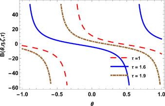
Fig.1 2D Graphics.

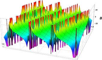
View original graphic|Download|PPT slide

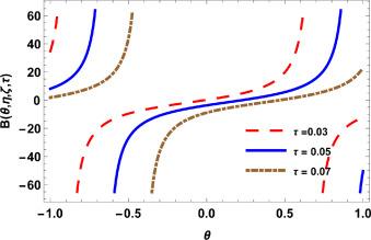
Fig.2 3D Graphics. Graphical interpretation of $B_{1, 2} (θ, η, ζ, τ)$ for $κ_{1} = 1$ , $κ_{3} = 0.75$ , $ν = 2.00$ , $γ = 2$ , $μ = 3.00$ , $ω = 4$ , $ν = 2$ and $Ω = 1$ , $c = - 90.5$ .

View original graphic|Download|PPT slide

Fig.3 2D Graphics.

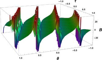
View original graphic|Download|PPT slide

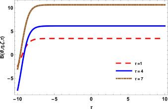
Fig.4 3D Graphics. Graphical interpretation of $B_{1, 1} (θ, η, ζ, τ)$ for $κ_{1} = 1$ , $κ_{3} = 0.75$ , $ν = 2.00$ , $γ = 2$ , $μ = 3.00$ , $ω = 4$ , $ν = 2$ $Ω = 1$ , and $c = - 90.5$ .

View original graphic|Download|PPT slide

Fig.5 2D Graphics.

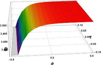
View original graphic|Download|PPT slide

Fig.6 3D Graphics. Graphical interpretation of $B_{2, 1} (θ, η, ζ, τ)$ for $κ_{1} = 1$ , $κ_{3} = 0.75$ , $ν = 2.00$ , $γ = 2$ , $μ = 3.00$ , $ω = 4$ , $Ω = 1$ , and $c = - 90.5$ .

In Fig. 7, Fig. 8, Fig. 9, Fig. 10, graphically behaviour of 3D and 2D presented for Eq. (86) for

κ_{1} = 1

κ_{3} = 0.5

ν = 1

κ_{2} = 1

γ = 1

μ = - 2

ω = 1

Ω = 2

, and

c = 1

. Graphically behaviour of 3D and 2D are presented for

B_{3, 1} (θ, η, ζ, τ)

in Figs. 11 and 12.

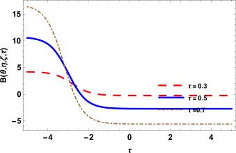
View original graphic|Download|PPT slide

Fig.7 2D Graphics.

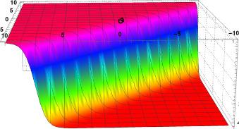
View original graphic|Download|PPT slide

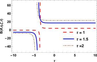
Fig.8 3D Graphics. Graphical interpretation of $B_{4, 1} (θ, η, ζ, τ)$ for $κ_{1} = 1$ , $κ_{3} = 0.5$ , $ν = 1$ , $κ_{2} = 1$ , $γ = 1$ , $μ = - 2$ , $ω = 1$ , $Ω = 2$ , and $c = 1$ .

View original graphic|Download|PPT slide

Fig.9 2D Graphics.

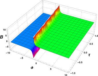
View original graphic|Download|PPT slide

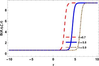
Fig.10 3D Graphics. Graphical interpretation of $B_{4, 2} (θ, η, ζ, τ)$ for $κ_{1} = 1$ , $κ_{3} = 0.5$ , $ν = 1$ , $κ_{2} = 1$ , $γ = 1$ , $μ = - 2$ , $ω = 1$ , $Ω = 2$ , and $c = 1$ .

View original graphic|Download|PPT slide

Fig.11 2D Graphics.

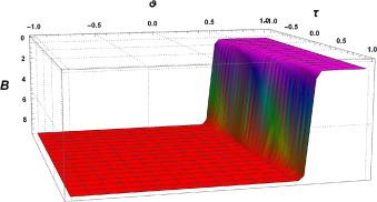
View original graphic|Download|PPT slide

Fig.12 3D Graphics. Graphical interpretation of $B_{3, 1} (θ, η, ζ, τ)$ for $κ_{1} = 1$ , $κ_{3} = 0.05$ , $ν = 3$ , $κ_{2} = 1$ , $γ = 2$ , $μ = 1$ , $ω = 0.75$ , $Ω = 2$ , and $c = 2$ .

Figs. 13 -16 shows the different graphically behaviours of Eq. (87) for

κ_{1} = 1

κ_{3} = 2

ν = 3

γ = 4

μ = 5

ω = 1

and

Ω = 1

c = - 20.5

. We have showed the graphical representation of Eq. (88) for

κ_{1} = 1

κ_{3} = 2.5

ν = 1.00

γ = 2

μ = 1.00

ω = 2

Ω = 1

ν = 1

and

c = - 4.5

in Fig. 17, Fig. 18, Fig. 19, Fig. 20. and also

B_{7, 1} (θ, η, ζ, τ)

shows graphically structure for

κ_{1} = 1

κ_{3} = 0.95

ν = 1

κ_{2} = 1

γ = 0

ν = 1

μ = 3

ω = 7

and

Ω = 2

c = - 44.5

in Fig. 21 and 22.graphically behaviours of

B_{9, 1} (θ, η, ζ, τ)

for

κ_{1} = 1

κ_{3} = 2

ν = 1

κ_{2} = 1

γ = 3

ν = 1

μ = 3

ω = 3

and

Ω = 1

c = - 18

in Fig. 23 and 24.

View original graphic|Download|PPT slide

Fig.13 2D Graphics.

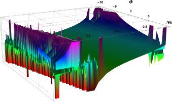
View original graphic|Download|PPT slide

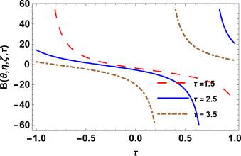
Fig.14 3D Graphics. Graphical interpretation of $B_{5, 1} (θ, η, ζ, τ)$ for $κ_{1} = 1$ , $κ_{2} = 1$ , $κ_{3} = 2$ , $ν = 3$ , $γ = 4$ , $μ = 5$ , $ω = 1$ , $Ω = 1$ , and $c = - 20.5$ .

View original graphic|Download|PPT slide

Fig.15 2D Graphics.

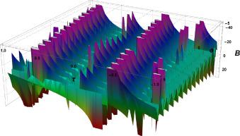
View original graphic|Download|PPT slide

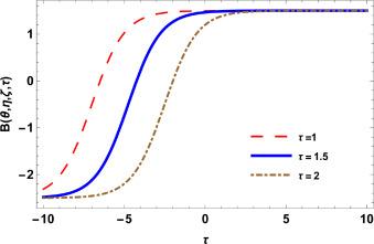
Fig.16 3D Graphics. Graphical interpretation of $B_{5, 2} (θ, η, ζ, τ)$ for $κ_{1} = 1$ , $κ_{3} = 2$ , $ν = 3$ , $γ = 4$ , $μ = 5$ , $ω = 1$ , $κ_{2} = 1$ $Ω = 1$ , and $c = - 20.5$ .

View original graphic|Download|PPT slide

Fig.17 2D Graphics.

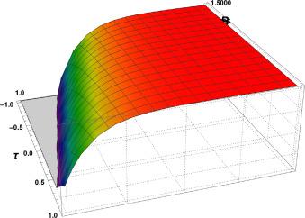
View original graphic|Download|PPT slide

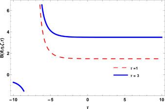
Fig.18 3D Graphics. Graphical interpretation of $B_{6, 1} (θ, η, ζ, τ)$ for $κ_{1} = 1$ , $κ_{3} = 2.5$ , $ν = 1.00$ , $γ = 2$ , $μ = 1.00$ , $ω = 2$ $Ω = 1$ , $ν = 1$ , and $c = - 4.5$ .

View original graphic|Download|PPT slide

Fig.19 2D Graphics.

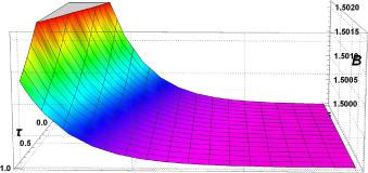
View original graphic|Download|PPT slide

Fig.20 3D Graphics. Graphical interpretation of $B_{6, 2} (θ, η, ζ, τ)$ for $κ_{1} = 1$ , $κ_{3} = 2.5$ , $ν = 1.00$ , $γ = 2$ , $μ = 1.00$ , $ω = 2$ $Ω = 1$ , $ν = 1$ , and $c = - 4.5$ .

View original graphic|Download|PPT slide

Fig.21 2D Graphics.

View original graphic|Download|PPT slide

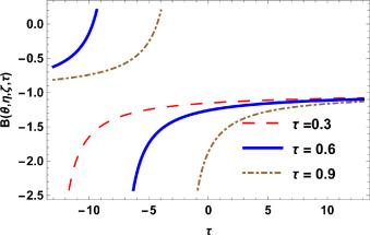
Fig.22 3D Graphics. Graphical interpretation of $B_{7, 1} (θ, η, ζ, τ)$ for $κ_{1} = 1$ , $κ_{3} = 0.95$ , $ν = 1$ , $κ_{2} = 1$ , $γ = 0$ , $ν = 1$ $μ = 3$ , $ω = 7$ , $Ω = 2$ , and $c = - 44.5$ .

View original graphic|Download|PPT slide

Fig.23 2D Graphics.

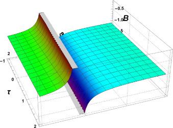
View original graphic|Download|PPT slide

Fig.24 3D Graphics. Graphical interpretation of $B_{9, 1} (θ, η, ζ, τ)$ for $κ_{1} = 1$ , $κ_{3} = 2$ , $ν = 1$ , $κ_{2} = 1$ , $γ = 3$ , $ν = 1$ , $μ = 3$ , $ω = 3$ , $Ω = 1$ , and $c = - 18$ .

Figs. 25 and 26 shows the graphically behaviours of

B_{14, 1} (θ, η, ζ, τ)

for

κ_{1} = 0.75

κ_{3} = 3

ν = 1

κ_{2} = 1

γ = 3

ν = 1

μ = 0

ω = 2

and

Ω = 1

c = 1.45

B_{15, 1} (θ, η, ζ, τ)

shows graphically representation for

κ_{1} = 0.9

κ_{3} = 0.75

ν = 2

κ_{2} = 1

γ = 3

μ = 3

ω = 3

Ω = 2

, and

c = - 57.1

in Fig. 27 and 28.

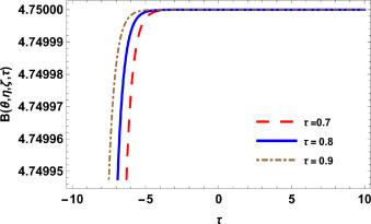
View original graphic|Download|PPT slide

Fig.25 2D Graphics.

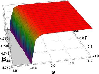
View original graphic|Download|PPT slide

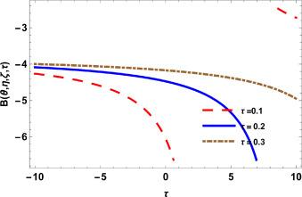
Fig.26 3D Graphics. Graphical interpretation of $B_{14, 1} (θ, η, ζ, τ)$ for $κ_{1} = 0.75$ , $κ_{3} = 3$ , $ν = 1$ , $κ_{2} = 1$ , $γ = 3$ , $μ = 0$ , $ω = 2$ , $Ω = 1$ , and $c = 1.45$ .

View original graphic|Download|PPT slide

Fig.27 2D Graphics.

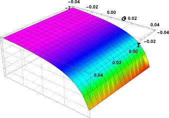
View original graphic|Download|PPT slide

Fig.28 3D Graphics. Graphical interpretation of $B_{15, 1} (θ, η, ζ, τ)$ for $κ_{1} = 0.9$ , $κ_{3} = 0.75$ , $ν = 2$ , $κ_{2} = 1$ , $γ = 3$ , $μ = 3$ , $ω = 3$ , $Ω = 2$ , and $c = - 57.1$ .

5. Conclusion

Exact and solitons solutions to the (

3 + 1

)-dimensional Gardner-KP equation are analyzed using a hybrid method consisting of the Lie symmetry method and the new auxiliary equation method. These techniques are still encouraging for developing multiple periodic and soliton solutions to the model under consideration that have not been reported in the published literature. The application of the new auxiliary equation method can get a large number of distinct accurate solutions to the governing equation. The results of this study are significant to both physicists and mathematicians because the multi-dimensions Gardner-KP equation indicates strongly nonlinear internal waves on ocean shelves in two-dimensional instances. Also, weakly nonlinear, dispersive surface waves propagating near-critical depth levels were shown to be governed by the Gardner-KP equation. The new exact solutions to this equation having many applications in different fields will provide insight to mathematicians and physicists to study more nonlinear models.

Declaration of Competing Interest

Authors declare that they have no conflict of interest.

Acknowledgment

The authors would like to thank the Deanship of Scientific Research at Majmaah University for supporting this work under Project R-2022-178.

References

Publishing order | Descend order by publishing year | Descend order by cited within

[1]	A. Zafar, M. Shakeel, A. Ali, L. Akinyemi, H. Rezazadeh. Opt. Quantum Electron., 54 (5) (2022), pp. 1-15 DOI: 10.53963/pjmr.2022.006.4

[2]	L. Akinyemi, U. Akpan, P. Veeresha, H. Rezazadeh, M. Inc. J. Ocean Eng. Sci. (2022)In Press

[3]	A. Hussain, M. Junaid-U-Rehman, F. Jabeen, I. Khan. Int. J. Geom. Methods Mod. Phys., 19 (5) (2022), p. 2250075

[4]	K. Debin, H. Rezazadeh, NajibUllah, J. Vahidide, K.U. Tariq, L. Akinyemi. J. Ocean Eng. Sci. (2022)In Press

[5]	L. Akinyemi, M. Inc, M.M.A. Khater, H. Rezazadeh. Opt. Quantum Electron., 54 (191) (2022), pp. 1-15 DOI: 10.15388/namc.2022.27.26374

[6]	A. H. Arnous, M. Mirzazadeh, L. Akinyemi, A. Akbulut. J. Ocean Eng. Sci. (2022)In Press

[7]	I.E. Inan, M. Inc, H. Rezazadeh, L. Akinyemi. Opt. Quantum Electron., 54 (261) (2022), pp. 1-15 DOI: 10.4324/9781003165705-1

[8]	S. Watanabe. J. Phys. Soc. Jpn., 53 (1984), pp. 950-956

[9]	M.S. Ruderman, T. Talipova, E. Pelinovsky. J. Plasma Phys., 74 (2008), pp. 639-656 DOI: 10.1017/s0022377808007150

[10]	A.M. Kamchatnov, Y.V. Kartashov, P.-E. Larre, N. Pavloff. Phys. Rev. A., 89 (2014), p. 033618 DOI: 10.1103/PhysRevA.89.033618

[11]	G. Aslanova, S. Ahmetolan, A. Demirci. Phys. Rev. E., 102 (2020), p. 052215

[12]	Y. Chen, P.L.F. Liu. Wave Motion, 27 (3) (1988), pp. 321-339

[13]	G. Aslanova, S. Ahmetolan, A. Demirci. Phys. Rev. E., 102 (2020), p. 052215

[14]	K.U. Tariq, A.R. Seadawy, S.Z. Alamri. Pramana J. Phys, 91 (68) (2018), pp. 1-13

[15]	K. Boateng, W. Yang, D. Yaro, M.E. Otoo. Math. Methods Appl. Sci., 43 (2020), pp. 3457-3472 DOI: 10.1002/mma.6131

[16]	A.M. Wazwaz. Appl. Math. Comput., 204 (2008), pp. 162-169

[17]	G. Aslanova, A. Demirci, S. Ahmetolan. Wave Motion, 109 (2022), p. 102844

[18]	M.M.A. Khater, A. R. Seadawy, D.C. Lu. Results Phys., 7 (2017), pp. 2325-2333

[19]	P.J. Olver. Applications of Lie Groups to Differential Equations. Springer, Berlin (1986)

[20]	G.W. Bluman, A.F. Cheviakov, S.C. Anco. Applications of Symmetry Methods to Partial Differential Equations. Springer, Berlin (2000)

[21]	M. Niwas, S. Kumar, H. Kharbanda. J. Ocean Eng. Sci., 7 (2022), pp. 188-201

[22]	A. Jhangeer, A. Hussain, M. J-U-Rehman, I. Khan, D. Baleanu, K.S. Nisar. Results Phys., 19 (2020), pp. 103-492

[23]	M.B. Riaz, A. Jhangeer, K.M. Abualnaja, M. Junaid-U-Rehman. Phys. Scr., 96 (2021), p. 104013 DOI: 10.1088/1402-4896/ac0dfe

[24]	A. Hussain, A. Jhangeer, N. Abbas. Int. J. Geo. Methods Mod. Phys., 18 (5) (2021), p. 2150071 DOI: 10.1142/s0219887821500717

[25]	R. Al-Deiakeh, O.A. Arqub, M. Al-Smadi, S. Momani. J. Ocean Eng. Sci. (2021)

[26]	C. Li, J. Zhang. Symmetry, 11 (5) (2019), p. 601

[27]	A. Hussain, S. Bano, I. Khan, D. Baleanu, K.S. Nisar. Symmetry, 12 (1) (2020), p. 170 DOI: 10.3390/sym12010170

[28]	Z. Zhao, L. He. Theor. Math. Phys., 206 (2021), pp. 142-162 DOI: 10.1134/s0040577921020033

[29]	A. Jhangeer, A. Hussain, M.J. Rehman, D. Baleanu, M.B. Riaz. Chaos, Solitons Fractals, 143 (2021), p. 11057

[30]	A. Hussain, A. Jhangeer, N. Abbas, I. Khan, K.S. Nisar. Ain Shams Eng. J., 12 (4) (2021), pp. 3919-3930

[31]	S. Kumar, I. Hamid, M.A. Abdou. J. Ocean Eng. Sci.(2021) In Press

[32]	X. Hu, Y. Li, Y. Chen. J. Math. Phys., 56 (5) (2015), p. 053504

[33]	M.B. Riaz, J. Awrejcewicz, A. Jhangeer, M. Junaid-U-Rehman, Y.S. Hamed, K.M. Abualnaja. Eur. Phys. J. Plus, 137 (2022), pp. 1-18 DOI: 10.1155/2022/3664302

Options

Outlines

模态框（Modal）标题

Abstract

Cite this article

1. Introduction

2. Lie symmetry analysis of Eq. (1)

2.1. Symmetry groups

3. One-dimensional optimal system

3.1. Calculation of the invariants

Table 1 Commutator table .

3.2. Construction of the adjoint transformation matrix

Table 2 Adjoint representation table.

3.3. Optimal system

3.4. Similarity reductions and exact solutions

4. Soliton solutions

4.1. Similarity reduction from translational symmetries

4.2. Solutions of Eq. (78) by new auxiliary method

4.3. Graphical results

4.3.1. Graphic description

Fig.1 2D Graphics.

Fig.2 3D Graphics. Graphical interpretation of B1,2(θ,η,ζ,τ) for κ1=1 , κ3=0.75 , ν=2.00 , γ=2 , μ=3.00 , ω=4 , ν=2 and Ω=1 , c=−90.5 .

Fig.3 2D Graphics.

Fig.4 3D Graphics. Graphical interpretation of B1,1(θ,η,ζ,τ) for κ1=1 , κ3=0.75 , ν=2.00 , γ=2 , μ=3.00 , ω=4 , ν=2 Ω=1 , and c=−90.5 .

Fig.5 2D Graphics.

Fig.6 3D Graphics. Graphical interpretation of B2,1(θ,η,ζ,τ) for κ1=1 , κ3=0.75 , ν=2.00 , γ=2 , μ=3.00 , ω=4 , Ω=1 , and c=−90.5 .

Fig.7 2D Graphics.

Fig.8 3D Graphics. Graphical interpretation of B4,1(θ,η,ζ,τ) for κ1=1 , κ3=0.5 , ν=1 , κ2=1 , γ=1 , μ=−2 , ω=1 , Ω=2 , and c=1 .

Fig.9 2D Graphics.

Fig.10 3D Graphics. Graphical interpretation of B4,2(θ,η,ζ,τ) for κ1=1 , κ3=0.5 , ν=1 , κ2=1 , γ=1 , μ=−2 , ω=1 , Ω=2 , and c=1 .

Fig.11 2D Graphics.

Fig.12 3D Graphics. Graphical interpretation of B3,1(θ,η,ζ,τ) for κ1=1 , κ3=0.05 , ν=3 , κ2=1 , γ=2 , μ=1 , ω=0.75 , Ω=2 , and c=2 .

Fig.13 2D Graphics.

Fig.14 3D Graphics. Graphical interpretation of B5,1(θ,η,ζ,τ) for κ1=1 , κ2=1 , κ3=2 , ν=3 , γ=4 , μ=5 , ω=1 , Ω=1 , and c=−20.5 .

Fig.15 2D Graphics.

Fig.16 3D Graphics. Graphical interpretation of B5,2(θ,η,ζ,τ) for κ1=1 , κ3=2 , ν=3 , γ=4 , μ=5 , ω=1 , κ2=1 Ω=1 , and c=−20.5 .

Fig.17 2D Graphics.

Fig.18 3D Graphics. Graphical interpretation of B6,1(θ,η,ζ,τ) for κ1=1 , κ3=2.5 , ν=1.00 , γ=2 , μ=1.00 , ω=2 Ω=1 , ν=1 , and c=−4.5 .

Fig.19 2D Graphics.

Fig.20 3D Graphics. Graphical interpretation of B6,2(θ,η,ζ,τ) for κ1=1 , κ3=2.5 , ν=1.00 , γ=2 , μ=1.00 , ω=2 Ω=1 , ν=1 , and c=−4.5 .

Fig.21 2D Graphics.

Fig.22 3D Graphics. Graphical interpretation of B7,1(θ,η,ζ,τ) for κ1=1 , κ3=0.95 , ν=1 , κ2=1 , γ=0 , ν=1 μ=3 , ω=7 , Ω=2 , and c=−44.5 .

Fig.23 2D Graphics.

Fig.24 3D Graphics. Graphical interpretation of B9,1(θ,η,ζ,τ) for κ1=1 , κ3=2 , ν=1 , κ2=1 , γ=3 , ν=1 , μ=3 , ω=3 , Ω=1 , and c=−18 .

Fig.25 2D Graphics.

Fig.26 3D Graphics. Graphical interpretation of B14,1(θ,η,ζ,τ) for κ1=0.75 , κ3=3 , ν=1 , κ2=1 , γ=3 , μ=0 , ω=2 , Ω=1 , and c=1.45 .

Fig.27 2D Graphics.

Fig.28 3D Graphics. Graphical interpretation of B15,1(θ,η,ζ,τ) for κ1=0.9 , κ3=0.75 , ν=2 , κ2=1 , γ=3 , μ=3 , ω=3 , Ω=2 , and c=−57.1 .

5. Conclusion

Declaration of Competing Interest

Acknowledgment

References

Links

Fig.2 3D Graphics. Graphical interpretation of $B_{1, 2} (θ, η, ζ, τ)$ for $κ_{1} = 1$ , $κ_{3} = 0.75$ , $ν = 2.00$ , $γ = 2$ , $μ = 3.00$ , $ω = 4$ , $ν = 2$ and $Ω = 1$ , $c = - 90.5$ .

Fig.4 3D Graphics. Graphical interpretation of $B_{1, 1} (θ, η, ζ, τ)$ for $κ_{1} = 1$ , $κ_{3} = 0.75$ , $ν = 2.00$ , $γ = 2$ , $μ = 3.00$ , $ω = 4$ , $ν = 2$ $Ω = 1$ , and $c = - 90.5$ .

Fig.6 3D Graphics. Graphical interpretation of $B_{2, 1} (θ, η, ζ, τ)$ for $κ_{1} = 1$ , $κ_{3} = 0.75$ , $ν = 2.00$ , $γ = 2$ , $μ = 3.00$ , $ω = 4$ , $Ω = 1$ , and $c = - 90.5$ .

Fig.8 3D Graphics. Graphical interpretation of $B_{4, 1} (θ, η, ζ, τ)$ for $κ_{1} = 1$ , $κ_{3} = 0.5$ , $ν = 1$ , $κ_{2} = 1$ , $γ = 1$ , $μ = - 2$ , $ω = 1$ , $Ω = 2$ , and $c = 1$ .

Fig.10 3D Graphics. Graphical interpretation of $B_{4, 2} (θ, η, ζ, τ)$ for $κ_{1} = 1$ , $κ_{3} = 0.5$ , $ν = 1$ , $κ_{2} = 1$ , $γ = 1$ , $μ = - 2$ , $ω = 1$ , $Ω = 2$ , and $c = 1$ .

Fig.12 3D Graphics. Graphical interpretation of $B_{3, 1} (θ, η, ζ, τ)$ for $κ_{1} = 1$ , $κ_{3} = 0.05$ , $ν = 3$ , $κ_{2} = 1$ , $γ = 2$ , $μ = 1$ , $ω = 0.75$ , $Ω = 2$ , and $c = 2$ .

Fig.14 3D Graphics. Graphical interpretation of $B_{5, 1} (θ, η, ζ, τ)$ for $κ_{1} = 1$ , $κ_{2} = 1$ , $κ_{3} = 2$ , $ν = 3$ , $γ = 4$ , $μ = 5$ , $ω = 1$ , $Ω = 1$ , and $c = - 20.5$ .

Fig.16 3D Graphics. Graphical interpretation of $B_{5, 2} (θ, η, ζ, τ)$ for $κ_{1} = 1$ , $κ_{3} = 2$ , $ν = 3$ , $γ = 4$ , $μ = 5$ , $ω = 1$ , $κ_{2} = 1$ $Ω = 1$ , and $c = - 20.5$ .

Fig.18 3D Graphics. Graphical interpretation of $B_{6, 1} (θ, η, ζ, τ)$ for $κ_{1} = 1$ , $κ_{3} = 2.5$ , $ν = 1.00$ , $γ = 2$ , $μ = 1.00$ , $ω = 2$ $Ω = 1$ , $ν = 1$ , and $c = - 4.5$ .

Fig.20 3D Graphics. Graphical interpretation of $B_{6, 2} (θ, η, ζ, τ)$ for $κ_{1} = 1$ , $κ_{3} = 2.5$ , $ν = 1.00$ , $γ = 2$ , $μ = 1.00$ , $ω = 2$ $Ω = 1$ , $ν = 1$ , and $c = - 4.5$ .

Fig.22 3D Graphics. Graphical interpretation of $B_{7, 1} (θ, η, ζ, τ)$ for $κ_{1} = 1$ , $κ_{3} = 0.95$ , $ν = 1$ , $κ_{2} = 1$ , $γ = 0$ , $ν = 1$ $μ = 3$ , $ω = 7$ , $Ω = 2$ , and $c = - 44.5$ .

Fig.24 3D Graphics. Graphical interpretation of $B_{9, 1} (θ, η, ζ, τ)$ for $κ_{1} = 1$ , $κ_{3} = 2$ , $ν = 1$ , $κ_{2} = 1$ , $γ = 3$ , $ν = 1$ , $μ = 3$ , $ω = 3$ , $Ω = 1$ , and $c = - 18$ .

Fig.26 3D Graphics. Graphical interpretation of $B_{14, 1} (θ, η, ζ, τ)$ for $κ_{1} = 0.75$ , $κ_{3} = 3$ , $ν = 1$ , $κ_{2} = 1$ , $γ = 3$ , $μ = 0$ , $ω = 2$ , $Ω = 1$ , and $c = 1.45$ .

Fig.28 3D Graphics. Graphical interpretation of $B_{15, 1} (θ, η, ζ, τ)$ for $κ_{1} = 0.9$ , $κ_{3} = 0.75$ , $ν = 2$ , $κ_{2} = 1$ , $γ = 3$ , $μ = 3$ , $ω = 3$ , $Ω = 2$ , and $c = - 57.1$ .